 IST,
IST,
RBI WPS (DEPR): 17/2011: Why Persistent High Inflation Impedes Growth? An Empirical Assessment of Threshold Level of Inflation for India
| RBI Working Paper Series No. 17 Abstract *In the policy debate on growth-inflation tradeoff and the role of monetary policy in managing the tradeoff in the short-run, theoretical and empirical research suggests the presence of a country specific threshold level of inflation. Monetary policy may accommodate inflation up to the threshold level even when that is higher than the stated inflation target, but it must resist with clear commitment any increase in inflation beyond the threshold level because of the risks inflation itself could pose to growth. In other words, both inflation and growth objectives will be achieved by adopting and sustaining the anti-inflationary stance of monetary policy beyond the threshold. Empirical findings of this paper suggest that for India the threshold level of inflation could be around 6 per cent, which is consistent with the analyses of similar other studies for India in the past that indicate a range of 5 to 7 per cent. The inflation target for monetary policy may have to be somewhat lower than the growth maximizing threshold, since any positive inflation could be a risk to inclusive and sustainable growth objective, due to the unequal distribution of the benefits of growth and lack of hedge against inflation for a large section of the society. Thus, the welfare maximization goal would suggest the need for fixing a lower inflation target for policy purpose than the threshold, which however should not be too low to choke the grease effect of moderate inflation on growth. As per the assessment of this paper, the RBI’s inflation objective of containing the inflation perception in the range of 4 to 4.5 per cent is consistent with the need for balance between “growth maximizing threshold inflation” of about 6 per cent and “welfare maximizing low inflation” objective. The medium-term inflation objective of 3 per cent, consistent with India’s growing globalization, would have to result from productivity enhancing structural reforms and globalization induced efficiency gains, since monetary policy cannot alter either the potential rate of growth or the threshold inflation consistent with that rate of growth. JEL Classification: E 31, E 52. Key words: Growth-inflation trade-off, Threshold inflation, Backward-bending Phillips curve, Monetary policy response, Inflation target, Risks to growth. Introduction Growth-inflation tradeoff acquired centre stage of policy debate in India in 2011, as persistent high inflation coexisted with robust growth. The debate was particularly significant for the conduct of monetary policy of the RBI, as the emphasis of monetary policy had distinctly shifted course from “avoiding growth disruptive normalization” in 2010 to “containing inflation and anchoring inflation expectations” in 2011. Of the eleven successive increases in policy interest rates effected over the period March 2010 to July 2011, the first eight increases reflected normalization of the post-crisis monetary accommodation, and during this period one prominent aspect of the policy stance was to avoid disruptions to the growth momentum while gradually raising the anti-inflation accent simultaneously. During the subsequent three increases in policy rates in May, June and July 2011, however, the RBI clearly communicated the risk to medium-term growth from inflation as a justification for its policy actions. The Economic Survey, Government of India released in February 2011 created the impression that India may have to tolerate higher inflation if it has to aim at high growth. It specifically highlighted that “… we will, over the next 30 years, have an inflation rate that is 1.5 percentage points greater than would have been the case in the absence of this growth spurt…we will have an average annual inflation of nearly 5 per cent during the next decade or so of the rapid growth that is widely expected to occur in India”. The RBI, in turn, consistently highlighted its inflation objective as to “condition and contain perceptions of inflation in the range of 4.0 - 4.5 per cent, in line with the medium-term objective of 3.0 per cent inflation consistent with India’s broader integration into the global economy”. Moreover, it emphasized in its monetary policy statement of May 03, 2011 that “…based on cross-country as well as domestic experience, the Reserve Bank is strongly of the view that controlling inflation is imperative to sustaining growth over the medium-term”. The RBI reiterated its views more emphatically in the monetary policy statement on June 16, 2011: “…the monetary policy stance remains firmly anti-inflationary, recognizing that, in the current circumstances, some short-run deceleration in growth may be unavoidable in bringing inflation under control”. The risk of even potential growth being impacted adversely by high inflation was indicated in the policy statement of July 26, 2011: “…controlling inflation is imperative both for sustaining growth over the medium-term and for increasing the potential growth rate”. The July statement, thus, reflected what Friedman (1976) had highlighted about the possibility of inflation harming growth even in the long-run, unlike the position taken by Friedman (1968) earlier on the vertical shape of the Phillips Curve in the long-run. Moreover, even the short-run trade-off possibilities suggested by Friedman (1968) seem to hold only in the opposite direction beyond a threshold level of inflation. This realization is reflected in the growing emphasis on “low and stable inflation” as a necessary precondition to high, sustainable and inclusive growth. Against this backdrop, this paper aims at revisiting the growth-inflation tradeoff debate through specific empirical estimates of threshold inflation for India, taking into account the contemporary literature on the subject, as also common approaches to drawing policy relevant inferences from the empirical estimates. Section-II sets out the multiple channels through which inflation could hurt growth. Here the focus is on analytical reasoning, as a first layer justification for “why low and stable inflation is essential for high, sustainable and inclusive growth”. Cross country evidences are presented in brief in Section-III, which serves as the second layer justification. Section-IV documents how the theoretical debate on the growth-inflation tradeoff has evolved over time to the point of current overwhelming recognition of the fact that “beyond a threshold level of inflation the conventional Phillips Curve bends backward”. This also serves to provide the third layer of justification. Empirical estimation of threshold inflation for India is attempted in Section-V. Concluding observations are set out in Section-VI, with an assessment of inflation objective for monetary policy relative to the estimated threshold level. Section-II: Risks to Growth from Inflation – Some Obvious Triggers The adverse impact of inflation on growth could operate and manifest through multiple channels. Some of the important ones are presented here in brief. External Sector: Higher inflation and the resultant higher inflation differential relative to the inflation in rest of the world could cause the real effective exchange rate (REER) to appreciate, which in turn could weaken export growth. Moreover, domestic firms may find it difficult to pass on the rising input costs to consumers in the face of competition from cheaper imports, which may increase pressure on margins. Margin pressures could alter investment plans as well as cost of financing for firms. Private Investment: The most significant adverse impact of inflation could be on private investment and even productivity of investment1. First, firms have to spend time and money to understand and manage the effects of inflation on their business. Second, higher noise in the information embodied in prices could lead to over investment in some sectors and underinvestment in others2. Third, inflation could cause misallocation of financial resources - from productive investment to speculative activities. Fourth, it may discourage domestic savings3. Borrowers benefit at the expense of creditors in a rising inflation scenario. More debt than more savings could become the norm in a high inflation regime. Fifth, inflation could discourage capital inflows. Fiscal Imbalance: Even if inflation is seen as a tax, fiscal imbalances may actually increase in a high inflation environment. First, because of specific fiscal measures taken to contain inflation (such as tax cuts and higher subsidies), which in turn could delay fiscal consolidation. In the case of India, suppressed inflation could be significant, going by the magnitude of food, fertilizer and petroleum products subsidies. Second,expenditure growth at times may match inflation, given the indexation of wages and expected demands for compensation matching the rate of inflation. Revenue collection, however, may lag behind, due to lags in pricing of public utilities as well as incentives to underreport income to escape the inflation tax. Fiscal imbalance is a risk to both inflation and growth in the medium-run. Asset Prices: Stock markets may react adversely to high inflation, leading to negative wealth and income effects, as well as higher cost of funds, both of which could adversely impact growth. At times, however, asset price bubbles and associated positive wealth effect could become a source of inflationary pressures. Interest Rate: Anti inflationary monetary policy stance pursued in response to inflation could raise the cost of financing for investment and consumption activities, and thereby compress aggregate demand. Interest rate channel, however, may not be very effective when input cost pressures are passed on to consumers in the form of higher output prices, and consumers in general get wage increases matching the rate of inflation. Input Costs: When supply shocks increase input costs, that automatically raises headline inflation while simultaneously reducing growth. Supply shocks by their very nature lead to large relative price changes, which in turn may depress demand on the one hand while raising input costs on the other. The overall impact becomes visible in terms of low growth and high inflation. When repeated adverse supply shocks drive the inflation path, lower growth would co-exist with high headline inflation. Stagflationary possibilities could yield a growth-inflation relationship contrary to what the conventional Phillips Curve relationship suggests. At high inflation, the dispersion in relative prices increases, which in turn distorts price signals. The price of a good in a free market should be determined by its relative scarcity, i.e. supply relative to demand. But in a high inflation environment, relative price shifts may not reflect underlying demand-supply conditions of different goods and services. Because of this, market adjustments to distorted price signals may remain incomplete for long, impacting allocative efficiency of resources and economic growth. The urge for speculation as a means to escape the inflation induced erosion in purchasing power is another factor which impacts allocative efficiency. As highlighted by Cagan and Lipsey (1978), “…A high inflation rate generates massive economic waste…With market distortions rampant in a severe inflation, people able to do so concentrate on seeking fortunes by arbitraging the distortions. Inflation devastates the concept of economic value, generates resentment and cynicism, and sets continuing incentives for unethical business behaviour.” Coleman (2007) echoed similar risks from inflation and viewed that unpredictable inflation could transform “choices” into “gambles”. The quote he used from “Reflections on the Revolution in France” presents why inflation incentivizes speculative activities:
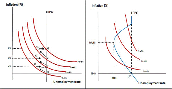
Section-III: Cross-country Evidence on the In the growth-inflation debate, given the risks to growth from inflation, a near consensus has evolved over time among central banks in terms of their emphasis on price stability as the dominant objective of monetary policy. As noted by Bernanke, et.al, (2007), “…One element of the new consensus is that low, stable inflation is important for market-driven growth”. How low then the inflation should be? Greenspan (2001) suggested in this context that “…price stability is best thought of as an environment in which inflation is so low and stable over time that it does not materially enter into the decisions of households and firms.” Fisher (1993) offered evidence on how macroeconomic stabilization, including control of inflation, is an important precondition for economic growth. In his cross-country analysis, he found that 1 percentage point increase in the rate of inflation could cost an economy more than one-tenth of a percentage point of growth. A subsequent stream of research emphasized that inflation may harm growth only when it crosses a threshold level (Sarel, 1996). Bruno and Easterly (1998) found this adverse impact of inflation on growth only at very high level of inflation (of 40 per cent), i.e. “an inflation crisis”. In turn, Judson and Orphanides (1996) and Hess and Moriss (1996) viewed that even at low levels of inflation it may retard growth significantly. Akerlof et al. (1996) showed why low inflation should be non-zero, as zero inflation involves higher unemployment/output costs compared to a positive low inflation of about 3 per cent (for the US). Empirical research involving cross country data, thus, suggests a wide range of possibilities. What is important to know, however, is that despite the use of alternative methodologies and different sample periods, all these studies corroborate the point that inflation harms growth, and that the threshold level matters. Barro (1995) studied the relationship using data for over 100 countries from 1960 to 1990, and found that increase in average inflation by 10 percentage points per year could involve a reduction in growth rate of real per capita GDP by 0.2 to 0.3 percentage points, besides a decrease in the ratio of investment to GDP by 0.4 to 0.6 percentage points. Thus, the private investment cycle could be impacted by inflation. Sarel (1995) examined the possibility of non-linear effects on economic growth, covering data for 87 countries for the period 1970 to 1990. It aimed at finding some answer to specific questions: (a) at what level of inflation the structural break occurs, (b) whether the break is significant, and (c) what could be the estimated values of the impact of inflation on growth. He found the break in his estimates at an inflation rate of 8 per cent. Below that rate, inflation may not have any impact on growth, or at best there may be marginal positive effect. At above 8 per cent, however, the adverse impact on growth was viewed as significant. This estimated threshold provided some guidance on why the inflation objective of a central bank may have to be below the threshold. The possibility of estimated threshold inflation being different for advanced and developing countries became evident from the study by Khan and Senhadji (2001). Covering a data set over the period 1960 to 1998 for 140 countries, their study suggested that the threshold level of inflation for developing countries could be higher at 11-12 per cent compared to about 1-3 per cent for the advanced economies. In empirical research on the non-linear growth-inflation relationship, it was viewed that once key determinants of growth are properly accounted for, then the apparent adverse impact of inflation on growth may decline. Ghosh and Phillips (1998) accordingly used a multivariate approach, covering data for 145 countries over the period 1960 to 1996. They found inflation to be a major determinant of growth, but with significant non-linear relationship. At inflation below 2 to 3 per cent a year or lower, inflation and growth exhibited a positive relationship. Above that level, not only the relationship appeared negative, but also convex, suggesting higher negative growth impact when inflation increases from say 10 per cent to 20 per cent compared to the increase from say 40 per cent to 50 per cent.They suggested a threshold level of 2.5 per cent4. Besides the level of inflation, inflation variability could also adversely impact growth. Jha and Dang (2011) examined the impact of inflation variability on economic growth using data for 182 developing countries and 31 developed countries over the period 1961 to 2009. They found that in developing countries when the rate of inflation exceeds 10 per cent, inflation variability adversely impacts growth. In the developed countries, however, no major evidence was found on the negative impact of inflation variability on growth. One obvious question that came up in the debate on threshold inflation is whether the inflation objective (or target) of a central bank should be aligned to the estimated threshold perfectly, or it should be below that? The cross country analysis of Christoffersen and Doyle (1998) provided some answer to this question. They found that disinflation from a moderate rate need not involve significant output costs. More importantly, countries closer to the threshold level of inflation do not aim to stay there without trying to converge to inflation levels of advanced economies. Similarly, for countries operating already at below the estimated threshold level of inflation, no evidence was found of growth increasing by moving closer towards the threshold with higher inflation. One major policy inference from the empirical research on threshold inflation then should be that inflation objective need not be set at the threshold level, since maximizing growth by allowing inflation up to the threshold level cannot be the sole objective of policy. Every level of inflation greater than zero involves erosion in purchasing power and harms a section of the population who may not have any hedge against inflation. When inflation becomes a risk to inclusive and sustainable growth, targeting growth maximizing inflation would not be appropriate, particularly when the benefits of growth do not get equally distributed. On the issue of threshold inflation versus inflation target, very little analysis is available on why inflation targets are set generally below the estimated threshold level. Wyplosz (2001) in this context had suggested in an article titled “Do We Know How Low Should Inflation Be?” that the ECB’s inflation target of 0 to 2 per cent could be well below the threshold of more than 5 per cent. The cost of this lower inflation target could possibly be a lower natural rate of unemployment by some 2 to 4 percentage points. Presenting this dilemma and suggesting the need for more work on the subject, he had viewed that “…the most reasonable conclusion seems that we do not know yet how low inflation should be.” Palley (2008) also had viewed in this context that empirical evidence for the US suggests it may attain the lowest unemployment rates when inflation remains in the range of 3 to 5 per cent, but the Fed is known to be guided by an inflation objective of not more than 2 per cent5. Akerlof et al. (2000) in fact presented empirical evidence of a threshold level of around seven percent. The available limited literature on estimated threshold inflation versus inflation target for conduct of monetary policy generally points to the trend of targets being invariably set below the estimated levels of threshold inflation. The other important dimension of the debate in the context of the estimated threshold level and inflation target is the need to accommodate temporary overshooting of the inflation path in the presence of supply shocks. Khan (2005) highlighted this dimension in his assessment of threshold for 26 MCD countries: “…maintaining inflation below 6 per cent does not preclude temporary deviations from a target …Developing countries are more prone to supply shocks…In the presence of downward nominal rigidities, monetary policies that do not accommodate supply shocks could amplify their adverse growth effects. This argues for setting (an implicit or explicit) inflation target as an average target over a medium-term horizon, which would then allow transitory deviations from it in order to accommodate first round effects.”6 Section-IV: Evolution of the Theoretical Debate on the Growth-Inflation Tradeoff The growth-inflation tradeoff debate started with an empirically observed relationship between change in money wages and the rate of unemployment over the period 1861-1913 in Great Britain (Phillips, 1958). The relationship was expected later to hold over the period 1913-57, which provided the first argument for “stability” in the relationship between these two variables. Being an empirically observed phenomenon, it was in search of a theory, which came first from Lipsey (1960) in the form of an excess demand model. It was essentially an inflation model, since rate of wage inflation was explained theoretically to depend on excess demand in the labour market. Around the same time, Samuelson and Solow (1960) suggested the scope for policy choice in this relationship, i.e. policy makers getting the option of a “menu of choice between different degrees of unemployment and price stability”. One important difference in these two approaches is that while the first one viewed inflation as an effect of labour market conditions (with excess demand influencing nominal wages), the second one seemed to suggest that policy makers have had the option to tolerate higher inflation for lowering the rate of unemployment (i.e. inflation could determine the rate of unemployment). The second view reflected essentially the Keynesian preference for policy activism, i.e. (involuntary) unemployment could be lowered by expanding demand through higher budget deficit or accommodative monetary policy. Increase in nominal demand could have dual effects; a real impact manifested in the form of higher output and a price impact in the form of higher inflation. Thus, there could be a positive relationship between inflation and unemployment, which could be exploited through active policy interventions. The extent to which an inflationary policy could be pursued to attain employment/ output goals and the existence of a possible threshold beyond which the positive relationship could either reverse or cease to exist represent the critical aspect of the subsequent theoretical debate on growth-inflation tradeoff. Six broad theoretical restatements of the Phillips Curve relationships7, as presented in Table-1, provide the essence of the debate. The first equation reflects the relationship as it started in the empirical observation of facts, i.e. a relationship between nominal wage and unemployment, but with one important difference, in terms of direction of causation. The wage rate is determined in this equation by the excess demand conditions in the labour market. If demand for labour exceeds supply, that will raise nominal wages. After the concept of natural rate of unemployment became known, employment gap (i.e. deviation of actual unemployment form natural unemployment level) was used as the determinant of inflation. If the unemployment rate falls below the natural rate, that could be a sign of excess demand for labour and overheating, thereby leading to higher inflation. Once this theoretical representation of Lipsey(1960) became available, interest in empirical tests started, which though suggested instability in the relationship, contrary to stable relationship propounded originally by Phillips. This prompted further advances in the theory of Phillips curve. In subsequent representations of the Phillips curve relationships, inflation (π) replaced wage rate (w), under the assumption of mark-up pricing (i.e. mark up over wage)8. Inflations expectations and their role in nominal wage adjustment process represented the key component of the re-statement of the Phillips Curve relationship by Friedman (1968) and Phelps (1968).Unlike static inflationary expectations of Lipsey (1960), Friedman and Phelps questioned the scope for stability in the relationship in an environment of changing inflationary expectations. In the short run, actual inflation could deviate from inflation expectations, and policy induced inflationary shocks could therefore yield positive output impact through money illusion. But inflation expectations are adaptive, and hence the illusion about a nominal increase in wages as a real increase could fade fast. At that point, the output impact will also disappear. The adaptive inflation expectation characterization of the Phillips Curve is presented in equation-2 in Table-1.This suggests that in the short run, π > πe, but in the long run, inflation expectations are fully realized (i.e. no illusion), and hence, π = πe. The typical graphical presentation of the shapes of the short-run and long-run Phillips curves reflecting this argument is in the first part of Chart-1. It shows that as inflation increases incrementally, at the given level of inflation expectations, the short-run trade-off possibility would yield a downward sloping short-run Phillips curve. The adaptive inflation expectation process, however, would ensure that inflation expectations catch up with higher inflation. The Phillips Curve in the long-run then will become vertical. Since π = πe in the long-run, u = u*; i.e. the actual unemployment rate is the same as the natural rate of unemployment (which later came to be known commonly as the NAIRU, to accommodate the time varying possibilities in the natural rate). Thus, policy activism to inflate nominal demand as a means to lower unemployment rate could work at best in the short-run, but not in the long-run. Accordingly, money could be non-neutral in the short-run, but it is neutral in the long run. One major policy inference from this argument is that natural rate of unemployment is independent of the inflation rate, i.e. u* ≠ f(π).9 Lucas (1972, 1973) replaced “adaptive expectations” with “rational expectations”, which seemed to suggest absence of any tradeoff between inflation and unemployment even in the short-run. In terms of equation-2 in Table-1, π = πe in both short-run and long-run. A corollary to this theoretical representation of the Phillips curve relationship was the emergence of literature emphasizing rule based monetary policy, time inconsistency problem in actual conduct of policy and the resultant loss of credibility, leading to subsequent focus on central bank independence. The possibility of a negatively sloped Phillips curve even in the long run was suggested by Tobin (1971). Equation-3 in Table-1 reflects this representation, in which the λπe segment is different from equation-2. Given the argument that 0<λ <1, this suggests that only part of the expected inflation gets fully reflected in actual inflation. Irrespective of whether expectations are adaptive or rational, this representation suggests that inflation expectations could get incorporated into nominal wage contracts only partly. Since incomplete incorporation of inflation expectations in wage contracts does not appear to be a credible phenomenon at the aggregate level, the justification came from the differences prevailing across sectors in terms of the extent of disequilibrium in the labour market and the degree of downward nominal wage rigidity. An inflationary policy shock engineered through higher nominal demand could encourage employment and output growth in sectors with unemployment, but raise inflation in sectors operating at full employment. As a result, the Phillips curve relationship will slope downwards, even when inflation is fully anticipated. This representation of the Phillips curve, being neo-Keynesian in nature, provided support for use of macro policy intervention to stabilize the economy. The multi-sector approach to explaining the tradeoff was elaborated further in Palley (1994, 1997), but with the emphasis on the point that the inflation expectations coefficient in equation-3 in Table-1 could be a function of the rate of unemployment. At higher rate of unemployment, most sectors may not resist decline in real wages resulting from inflation, which may be fully anticipated. As unemployment declines, however, resistance will increase, and expected inflation will be increasingly reflected in wage settings. When all sectors reach full employment, at that stage the Phillips curve will become vertical, because in all sectors anticipated inflation will be fully reflected in wage settings. This representation of the Phillips curve is presented in equation-4 in Table-1, in which the component λ(U)πe is different from the rest. This suggests that the coefficient λ is important, but unlike equation-3, here λ is a function of the rate of unemployment. This suggests that monetary policy could work till full employment is reached; but more importantly, it will work better when unemployment rate is high than low.When all sectors reach full employment, λ =1, and inflation expectations get fully incorporated in wage settings. The possibility of a back-ward bending Phillips curve was first suggested by Akerlof, Dickens and Schultz (2000).Unlike Tobin’s multi sector approach, this representation of the Phillps curve used a multi-agent framework, under which agents differ in their degrees of rationality. While some anticipate inflation rationally, others tend to underestimate. But as inflation increases, the percentage of underestimation falls.Thus, expected inflation is a function of inflation in this approach, which is captured in the πe(π) component in equation-5 of Table-1. When inflation increases from a low level, the conventional Phillips curve relationship holds. After a threshold level, however, the relationship reverses (second part of Chart-1).At some point, as the number of rational agents increases, unemployment increases. At very high inflation, all agents become rational, and the conventional long-run vertical Phillips curve holds. This representation provided the early leads on the existence of a threshold level of inflation, more particularly the fact that at different levels of inflation the unemployment-inflation tradeoff could change. Palley (2003) used a different approach to explain the backward bending nature of the relationship, using the earlier “multi-sector incomplete incorporation of inflation expectations” framework. In some sectors unemployment could be below full employment level and in others it could be at the full employment level. Wage-setting in response to expected inflation will vary across sectors. The most important aspect of Palley’s representation is the λ(πe)πe component in equation-6 of Table-1. Inflation expectations (πe) are incorporated in wage settings depending on the value of λ, but λ itself is a function of (πe). When inflation is low, expected inflation could also be low, and the degree to which expected inflation could be incorporated in wage settings may be far from complete. As inflation increases, the degree of inflation incorporation increases. Workers in increasing number of sectors resist inflation induced erosion in real wages, and accordingly the grease effect fades. The slopes of the short-run Phillips curves steepen for every successive higher inflation rate (please see second part of Chart-1).After a threshold level, “…the Phillips curve bends back because workers start to ratchet up their incorporation of inflation expectations faster than the increase in inflation”. (Palley, 2011) The shape of the Phillips curve for different levels of inflation will be the result of a family of short-run Phillips curves, each reflecting different degree of incorporation of expected inflation in wage settings. At some high inflation, the Phillips curve would become vertical. Unlike NAIRU, which represents the sustainable minimum unemployment rate, Palley’s Minimum Unemployment Rate of Inflation (MURI) represents the rate of inflation which is consistent with the minimum unemployment rate - MUR (or maximum output growth). In the empirical analysis of growth-inflation tradeoff, MURI could be equated with the threshold inflation.
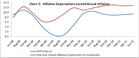
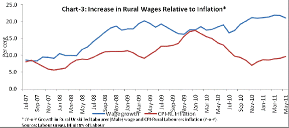
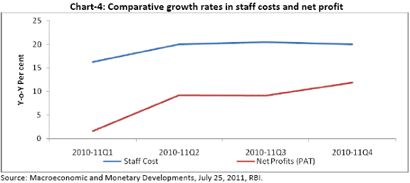
The above theoretical reasoning for backward bending possibilities in the unemployment-inflation relationship points to two factors as important preconditions for an empirical threshold relationship to exist. First, at some level of inflation, inflation expectations must exceed the actual inflation, and second, nominal wage increases must completely incorporate expected inflation. This would suggest a situation where input (including wage) costs rise faster than inflation, implying pressure on profit margins (since both input costs and profit margins cannot grow at a faster rate than inflation at the aggregate level).This pressure on profit margins could weaken investment demand, and hence yield the negative impact growth. As growth starts moderating, it may limit the degree to which inflation expectations could be incorporated in wages. But till such time, a kink will emerge in the inflation-growth relationship, providing justification for the existence of a threshold level of inflation. Thus, as inflation rises from a low level up to the threshold, inflation expectations will rise and the degree to which inflation expectations may get incorporated in wage contract will also increase. After the threshold, there will always be the risk of inflation expectations exceeding actual inflation, and for some time, wage increases may full reflect the higher expectations. The adverse impact on growth will start at that point. Available information for India suggests that inflation expectations (as per the RBI Survey data) have generally remained ahead of actual headline inflation, with lowest expectation seen in the recent years being about 6 per cent (Chart-2).More importantly, , the pace of increase in wages in rural and urban areas has also been much more than the inflation expectations in recent years. (Chart-3) Corporate finance data also suggest that growth in staff costs in recent quarters have been higher than the rate of growth in earnings (Table-2).These three trends corroborate the risks to growth from inflation, consistent with the theoretical arguments for backward bending Phillips curve.These trends also corroborate what Gokarn (2011) had highlighted as the plausible factors contributing to the kink in the growth-inflation tradeoff: “… The main reason for the existence of such a threshold rate of inflation is the speed and magnitude with which the inflation rate feeds into inflationary expectations. Below the threshold, workers and producers do not raise their wage and price demands very often because the impact of inflation is not too visible. By contrast, they respond very quickly above the threshold because they are worried that high inflation will rapidly erode their living standards or profitability. In short, when inflation is high, the behaviour of workers and producers increases the likelihood that it will increase further.”
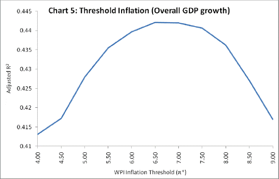
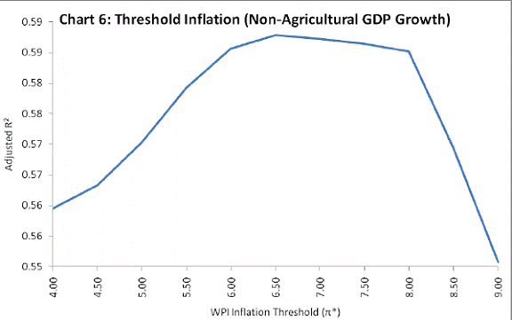
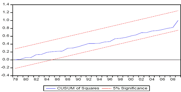
Section-V: Empirical Estimation of Threshold Inflation for India Threshold inflation is not a new concept to empirical research in India. Different studies for India point to a threshold inflation in the range of 5 to 7 per cent (Table-2). As noted by Ahluwalia (2011), “…inflation beyond the tolerable level – usually put at 5 to 6 per cent by the government and 4 to 5 per cent by the RBI – is regressive and also distortionary, damaging both inclusion and growth”. Given that both “high growth” and “inclusive growth” objectives face risks from high inflation, ensuring an inflation regime that does not yield higher than threshold inflation over successive months becomes an important policy objective. Like inflation exceeding threshold, at very low inflation also risks to both growth and inclusive growth objectives could start to emerge. If the grease effect of low inflation is hindered by targeting a very low inflation, that in turn could involve some growth sacrifice. While a very low inflation could be ideal for inclusive growth, the growth sacrifice from very low inflation may adversely impact the progress on inclusion. The comfort level of inflation indicated above, accordingly, reflects essentially perceived values of threshold inflation for India, as also the need to balance growth and inclusion objectives, given that both very high and very low inflation could be detrimental to both objectives. Three alternative methodologies are used in this paper to identify the threshold level of inflation for India. The first approach follows the most commonly used methodology suggested by Sarel (1995) and Khan and Senhadji (2000), i.e. spline regression, which allows a search process to detect the non-linearity in the relationship between inflation and growth, particularly the presence of a kink in the relationship. Since the value of the threshold (π*) is not known when the search process starts, after identifying the basic regression specification, equation is estimated as an iterative process by only changing the values of (π*) in small increments. At some point, the sum of squared residuals may be minimum (or Adjusted R2 maximum), and the corresponding value of the (π*) could then be taken as the threshold. While most of the studies presented in Table-2 have used this approach, some of them did not check for the stationarity of variables included in the regression equation, involving thereby the possibility of spurious regression. Moreover, the sample size and the variables selected in this paper are different from others. This paper also attempts to estimate threshold inflation for non agricultural GDP as well (assuming that high inflation may not adversely impact agricultural GDP as much as non-agricultural GDP). The basic equation for estimation is specified as GDPG= a0 + a1 D(Credit) + a2Monsoon +a3 (WPIInf)+ a4 D1(WPIInf-π*)+et ----- (1) Where GDPG=Growth in real GDP, D(Credit)= change in credit to GDP ratio, Monsoon=Deviation of monsoon rainfall from normal (as a proxy for supply shock), WPIInf=Inflation (WPI) and D1 = Dummy variable which takes value 1 if inflation is higher than threshold π* and 0 otherwise. In the estimated relationship, while a3 could capture the impact of inflation on growth, a4 would explain the impact of inflation exceeding threshold on growth. In the estimated equation, not only that both inflation and threshold variables should be statistically significant, but also that a3 should be positive and a4 should be negative. Another condition for the threshold level is that the sum of the two coefficients a3 and a4 should be negative above the threshold. While most other studies for India have used capital formation in the growth equation, this study use credit/GDP ratio, since from the stand point of monetary policy, this determinant of growth is important. Moreover, in a bank dominated financial system, credit could be a determinant of investment rate. To avoid the possibility of endogenity of credit relative to growth, credit/GDP ratio has been used, where the increase in the ratio largely reflects financial deepening. Deviation of monsoon from normal has to be seen as a supply shock and its impact on overall GDP growth is emphasized here, rather than only the impact on agricultural GDP, which is a part of the overall GDP. Omitted variables in the regression specification as also the possibility of structural breaks could be two possible sources of errors in estimating the threshold level. Quandt-Anderson test results for structural breaks suggest the absence of any statistically significant break-point in the relationship between growth and inflation in the sample period. CUSUM square test suggests the stability of estimated relationship in the regression, indicating thereby the absence of scope for errors on account of omitted variables (Annex Table 3 and Chart 1). The estimation is conducted for annual data over the period 1972-2010. The variables were tested for stationarity and the results are presented in Table 3. The estimated results for each level of threshold are presented in Annex Table 1. Since the important parameter in identifying the threshold inflation is the level of threshold at which the explanatory power of equation (1) and (2) becomes maximum, the Adjusted R2 is plotted against different levels of threshold in Chart 5 and 6, for both agricultural and non-agricultural GDP10.
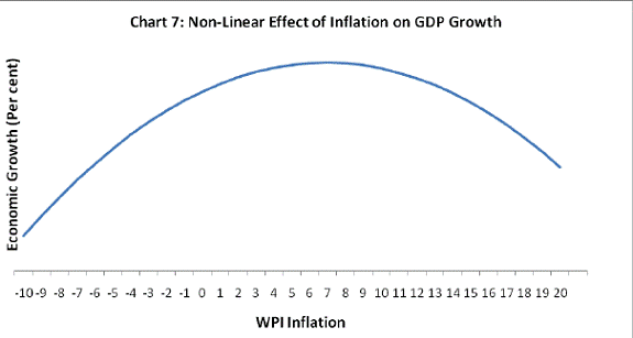
The pattern from the explanatory power of the regression equations (Adjusted R2) suggests that the grease effects of inflation almost ceases after 6 per cent level of inflation, which could ideally be considered as the estimated threshold level11. The results are more or less similar for both overall and non-agricultural GDP growth. In between 6 to 7.5 per cent range, the growth impact of inflation is insignificant (i.e. neither positive nor negative), which could therefore be seen as equivalent of the zone for “opportunistic policy response”, as outlined in Section-III. After 7.5 per cent inflation, the adverse impact on growth starts to increase, requiring sustained anti-inflation stance of monetary policy. The second approach used in this paper is a simple application of estimated relationship between growth and inflation, where the inflation variable itself captures the non-linearity, and the estimated coefficients from this regression are applied to different levels of inflation to identify the kink. Such models are still linear, but with non-linear variables. The following specification aims to capturing the presence of non-linearity between inflation and growth. GDPG=a0+ a1Monsoon+ a2(WPIInf) + a3(WPIInf)2+et ----- (3) Correspondingly, the estimated equation for India is given below: GDPG= 4.6 + 0.15Monsoon + 0.25WPIInf - 0.015(WPIInf)2 Using the estimated non-linear equation, a plot of the estimated economic growth at different levels of inflation is presented in Chart 7. The emphasis of the above equation is not to capture the impact of all possible determinants of growth, but only to identify the non-linearity in the relationship. Hence, rather than R-2, it is the signs of the WPIInf and (WPIInf)2 coefficients and the non-linear pattern in Chart-7 which are important for the assessment of threshold inflation.
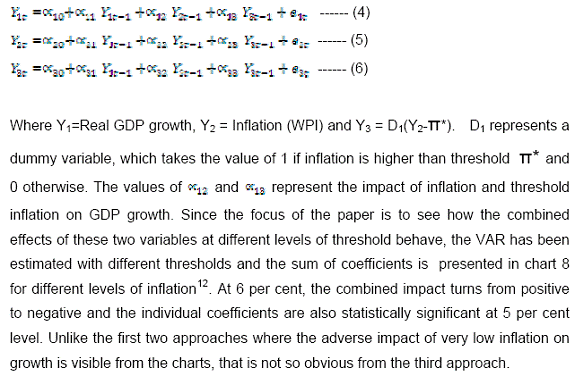
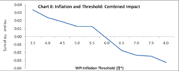
The results of the second approach more or less corroborate the findings of the first approach. As inflation increases from low level, the grease effect is distinctly visible. But beyond 6 per cent, the grease effects cease to exist. 6 to 8 per cent zone suggests indifference from policy standpoint, and hence, 6 could be preferred over 8, primarily due to larger welfare costs of 8 compared to 6 per cent. The third approach is a vector auto regression (VAR), where the steps are similar to the first approach, but lags of growth capture the impact of all other determinants of growth, and hence the focus remains only on the impact of inflation and threshold. As the VAR takes into account the lags of the dependant as well as the independent variables, the estimation would capture the dynamic nature of interaction between inflation and growth, which might not be captured in a simple OLS regression. One important dimension of the estimation of the threshold inflation is that the sum of coefficients of inflation and threshold inflation should turn from positive to negative beyond the threshold level of inflation. The identification of the threshold, thus, is guided by the point at which the combined impact of inflation and threshold (i.e. the sum of the two coefficients) turns from positive (or grease effects) to negative. This condition might not be realized in a static OLS estimation as it fails to take into account the lead lag relationship of inflation and growth, which is possible to test for this in a VAR framework. The basic specification of the VAR is as follows
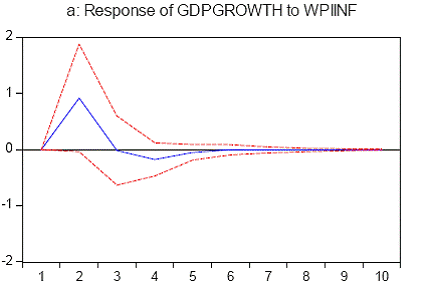
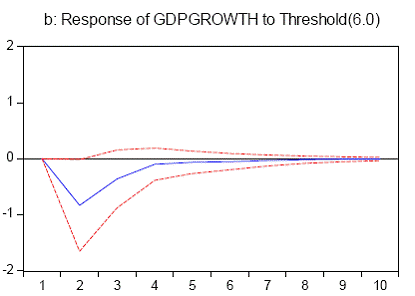
The impulse response of the VAR indicates that while inflation might give a positive shock to growth in the short run, it is more than offset by the negative shock from the threshold effect (Chart 9). While Chart 9.a shows that the impact of inflation could be positive on growth in the short run, Chart 9.b shows that once inflation is above the threshold, the adverse impact becomes distinctly visible.
Section-VI: Concluding Observations The grease effect of inflation for growth - as suggested by the conventional Phillips Curve – does not hold after a threshold level of inflation. If monetary policy tolerates somewhat higher inflation as a means to sustain high growth momentum, it may at some stage just become a sure path to sacrificing both inflation and growth objectives. The justification for inflation tolerance is often based on the perception of a positive relationship between inflation and growth, which fails to recognise the fact that the relationship invariably turns negative after a threshold level of inflation. The mainstream monetary policy emphasis on low and stable inflation reflects this realization; a central bank can best contribute to the growth objective by ensuring a low and stable inflation regime. In the empirical estimation of threshold inflation, because of the excessive emphasis on growth maximizing level of inflation, the welfare costs of inflation and risks to inclusive growth are often ignored. The inflation objective of a central bank, in turn, tries to balance both, by setting an inflation target which is below the estimated threshold. The inflation target accordingly is set not very far from the threshold to pose any risk to growth, but still lower than the threshold to minimize the welfare costs associated with any positive rate of inflation. This paper provides three layers of justifications to explain why high inflation impedes growth, drawing evidence from economic analysis, cross-country evidence and economic theory. Three alternative approaches were used to estimate the threshold level of inflation for India, besides exploring the non-linearity in the Phillips Curve relationship.Empirical estimates seem to suggest a growth maximizing inflation rate of about 6 per cent. It is also possible that the estimated threshold numbers may change over time, reflecting the changing structure of the economy and the sources of inflationary pressures. Past estimates of threshold inflation for India have been in the range of 5 to 7 percent, and one would have expected some moderation over the last decade, reflecting the benefits of reforms and globalization on inflation through higher productivity and competitive efficiency gains. Since the estimates of this paper continue to suggest a threshold of about 6 per cent, one would presume that persistent supply shocks would have neutralized the expected softening impact of globalization and reforms on the threshold level of inflation. RBI’s medium-term objective of 3.0 per cent inflation consistent with India’s broader integration into the global economy also reflects the normal expectations from reforms and globalization. If these valid expectations from reforms and globalization materialize, the corresponding threshold level would also decline over time. Recent experience, however, suggests that commodity price pressures have persisted, despite weak growth momentum in advanced economies. On the domestic front, growing demand supply imbalances in certain food items also reflect an emerging structural source of price pressure, which is unlikely to weaken fast. If food and energy prices together become a perpetual source of sequential or contemporaneous price pressure, it is unlikely that the threshold inflation would moderate to below 6 per cent level in the near-term. @ Sitikantha Pattanaik is Director and G V Nadhanael is Research Officer in the Department of Economic and Policy Research (DEPR). *They are grateful to Shri B.M Misra, Officer in Charge, DEPR and an anonymous referee for useful comments. Views presented in the paper are personal. The authors can be reached at spattanaik@rbi.org.in and nadhanael@rbi.org.in. 1Empirical findings of Li (2005) suggested that “…inflation has much more negative impact on the efficiency of investment than on the level of investment” in both developing and developed countries. He highlighted how the efficiency of investment (TFP growth) channel could be more important than the level of investment (capital accumulation) channel, even though most studies focus only on the latter. 2Relative price dispersion could be high when inflation is high. As noted by Beckerman (1992), when relative prices shift sharply and unsystematically “… the price system may inadequately reflect relative scarcities of goods and services, and so provide misleading, inappropriate signals to sellers and purchasers….Relative price dispersion, particularly in combination with price level uncertainty, causes problems for allocative efficiency and economic growth.” 3The composition of savings may also change, which will hinder availability of finance for investment. As underscored by Beckerman (1992), “…If wealth is held as gold, antique furniture, or foreign exchange, it is effectively removed from the economy’s financial circulation, and made unavailable to would be borrowers”. 4Li (2005) suggested the possible existence of a second threshold, above which the marginal effect of inflation on growth diminishes. For 90 developing countries over the period 1961-2004 estimates suggested the first threshold at 14 per cent, and the second threshold at 38 per cent. In between 14 and 38 per cent, the effect of inflation on growth is strongly negative and significant, but at rates above 38 per cent, the negative impact declines rapidly. 5Highlighting the difficulty that may be encountered while deciding on an inflation target relative to the estimated threshold inflation, Palley (2006) noted that “…if the public policy discussion is framed exclusively in terms of a two versus three per cent inflation target, the choice will naturally tend to be biased downward because inflation is a ‘bad’ so that that two per cent prima facie dominates three percent”. Accordingly, he viewed that the Fed need not adopt a formal explicit numerical inflation target and thereby avoid committing to a growth sacrifice that may naturally accompany a low inflation target . 6The distinction between “conventional” monetary policy response and “opportunistic” monetary policy response (depending on the level of inflation faced by a country relative to the threshold) is also important. As noted by Orphanides and Wilcox (1996), when prices are either rising rapidly or falling rapidly, there is no difference in the approach that may be adopted by a conventional policy maker and an opportunistic policy maker. However, when the rate of inflation is positive but not very high (relative to the target), a “reactive” stance as opposed to “pro-active” stance could be necessary, which would be typical of an opportunistic policy response. “…when inflation is moderate…the strategy involves waiting for external circumstances to deliver reductions in inflation, and in the meantime merely attempting to hold the line against upticks in inflation”. 7The option of using higher inflation as a means to support higher growth was rarely exercised in practice by central banks, even at the peak of the influence of Phillips Curve on policy makers. Highlighting this aspect, Forder (2008) noted that “…The Phillips curve was put to various uses, but advocating inflation was hardly amongst them….inflation advocacy did occur, it was rather rare; usually restricted to those with little influence”. 8 Instead of unemployment -gap, output-gap is often used in most empirical research, with the Okun Law (inverse) relationship between output growth and unemployment providing the transition. Accordingly, a conventional Phillips Curve interpretation would suggest a “positive” relationship between inflation and output growth, which is similar to an “inverse” relationship between inflation and unemployment. Similarly, a positive output gap could be associated with high inflation, whereas a positive unemployment gap could be associated with lower inflation. 9 Two important aspects of Friedman’s contribution to the policy debate are often ignored: (a) The scope for short-run trade off does not imply that policy makers can use it to the advantage of the economy through discretionary policies. The preferred option, therefore, could be a rule based money growth framework. As highlighted by Friedman (1968), “…The best course of action is to rely on the equilibrating forces of the market, imperfect as they may be, and on the stability of money demand, imperfect as it too may be, rather than seek a better approximation to perfection through “fine-tuning” policy”. (b) The scope for positive sloping Phillps Curve, i.e. a positive relationship between inflation and unemployment, consistent with the outcome in a stagflation. Highlighting how “scientific theories are revised”, Friedman (1976) noted that just like the negatively sloped Phillips Curve in the short-run, “…a positively sloped Phillips curve over somewhat longer periods may occur as a transitional phenomenon”, suggesting the continued relevance of the natural rate concept. But the transition phase for the upward sloping relationship could be little longer than the downward sloping Phillips curve relationship, and that explains the risk higher inflation could pose to growth and employment. As stressed by Bernanake et al (2007), “…Because inflation inhibits economic growth and efficiency, an increase in inflation may in fact lead to slightly higher (rather than lower) unemployment in the long-run”. While Friedman (1976) did not mention explicitly that natural rate of unemployment will be impacted by inflation, his reference to longer transition period for the upward sloping relationship has to be read along with his emphasis that a higher and more volatile inflation would “…render the economic system less efficient, introduce frictions in all markets and very likely raise the recorded rate of unemployment”. Thus, while Friedman (1968) highlighted the vertical shape of the Phillips Curve in the long-run (i.e. unemployment rate is independent of inflation and monetary policy), Friedman (1976) viewed that in the long-run a positive relationship may exist between inflation and unemployment (unlike the negative relationship in the short run). Haug and King (2011) found strong evidence of such a long-run relationship for the US data over the period 1952 to 2010, with inflation leading unemployment by 3 to 3.5 years. 10Any estimate of threshold inflation could at best be an approximation, rather than precise. The dynamic process of interactions between growth and inflation could be too complex to be captured by any single approach of estimation. This paper, therefore, uses three alternative approaches of estimation, giving the emphasis on whether all of them point to a similar level of threshold for India. 11Besides maximum Adjusted R2 , another pre-requisite in the identification of the threshold level of inflation is whether the sum of signs of the inflation and threshold coefficients reverse signs at the threshold level. Recognising this limitation of the estimate of threshold based on the regression approach, an alternative approach using VAR has been used which satisfies the requirement of reversal of signs of the combined coefficients. 12The lag length of the VAR was selected on the basis of AIC and SIC criteria (as 1 lag), for 6 per cent threshold. For other threshold levels, the same lag length was retained, given the importance of the sum of the coefficients for this approach. Ideally, though, for each threshold, the optimal lag length should have come from AIC and SIC. References: Akerlof, G A, W T Dickens and G L Perry (1996), “The Macroeconomics of Low Inflation”, Brookings Papers on Economic Activity. “ (2000), “Near-rational wage and Price Setting and the Long-run Phillips Curve”, Brookings Papers on Economic Activity. Ahluwalia, Montek S (2011), “Prospects and Policy Challenges in the Twelfth Plan”, Economic and Political Weekly, May 21, 2011. Barro, R.J. (1995), “Inflation and Economic Growth”, NBER Working Paper No 5326. Beckerman, Paul (1992), “The Economics of High Inflation”, Macmillan. Bernanke, Ben S, Thomas Laubach, Frederic S. Mishkin and Adam S Posen (2007), “Inflation Targeting: Lessons from the International Experience”, New Age International Publishers, New Delhi. Bhanumurthy, N R and Dony Alex (2010), “ Threshold Level of Inflation for India”, Asian Profile, Vol. 38, No. 5, October. Bruno, M and Easterly (1995), “Inflation Crises and Long-Run Growth”, World Bank Policy Research Working Paper No 1517. Cagan, Phillip and Robert E Lipsey (1978),“The Financial Effects of Inflation”, NBER General Series No. 103. Christoffersen, P and P Doyle (1998), “From Inflation to Growth - Eight Years of Transition”, IMF Working Paper No. WP/98/100. Coleman, William Oliver (2007),“The Cause, Costs and Compensation of Inflation”, Edward Elgar. Fisher, S (1993), “The Role of Macroeconomic Factors in Growth”, NBER Working paper No 4565. Forder, James (2008), “Friedman’s Nobel Lecture Reconsidered”, University of Oxford, Department of Economics Discussion Paper No. 398, July. Friedman, Milton (1968), “The Role of Monetary Policy”, American Economic Review, Vol. 58. Friedman, Milton (1976), “Inflation and Unemployment”, Nobel Memorial Lecture, December 13. Greenspan, Allen (2001), “Transparency in Monetary Policy” remarks at the Federal Reserve Bank of St. Louis, Economic Policy Conference, 11 October. Ghosh, A and S Phillips (1998), “Warning: Inflation may be Harmful to your Growth”, IMF Staff Papers Vol. 45, No.4. Gokarn, Subir (2011), “Sustainbility of Economic Growth and Controlling Inflation: The Way Forward”, Address at FICCI’s National Executive Committee Meeting, Mumbai, April 5. Haug, Alfred A and Ian P. King(2011), “Empirical Evidence on Inflation and Unemployment in the Long-run”, Workshop on Macroeconomics and Dynamics, June 21. Jha, Raghbendra and Tu Dang (2011), “Inflation variability and the Relationship between Inflation and growth”, ASARC Working Paper 2011/08. Kalirajan, K P and Kanhaiya Singh (2003), “The Inflation-Growth Nexus in India: An Empirical Analysis”, Journal of Policy Modeling, Vol. 25. Kannan, R and Himanshu Joshi (1998), “Growth-Inflation Tradeoff: Empirical Estimation of Threshold Rae of Inflation for India”, Economic and Political Weekly, October 17-23/24-30. Khan, Mohsin (2005), “Inflation and Growth in MCD Countries”, Middle East and Central Asia Department, IMF, December 2. Khan, Mohsin and A S Senhadji (2001), “Threshold Effects in the Relationship between Inflation and Growth”, IMF Staff papers, Vol 48, No 1. Li, Min (2005), “Inflation and Economic Growth: Threshold Effects and Transmission Mechanisms”, Department of Economics, University of Alberta. Lucas Jr., R E (1973),“Some International Evidence on Output-inflation Tradeoffs”, American Economic Review, Vol. 63. “ (1972),“Expectations and the Neutrality of Money”, Journal of Economic Theory, 4. Lipsey, R G (1960), “The Relationship between Unemployment and the Rate of Change of Money Wage Rates in the United Kingdom”, 1862-1967: A Further Analysis”, Economica, 27. Mohanty, Deepak (2010), “Perspectives on Inflation in India”, Address at Bankers Club, Chennai, September 28. Orphanides, Athanasios and David W. Wilcox (1996), “The Opportunistic Approach to Disinflation”, Board of Governors of the Federal Reserve System, May. Palley, Thomas I (2003), “The Backward Bending Phillips Curve and the Minimum Unemployment Rate of Inflation”, The Manchester School Vol. 71, No.1, January. “ (2006), “The Economics of Inflation Targeting: Negatively Sloped, Vertical, and Backward Bending Phillips Curves”, Meeting of Eastern Economic Association, Philadelphia, February 24-26. “ (2008), “The Backward Bending Phillips Curves: A Simple Model”, Political Economy Research Institute Working Paper Number 168. “ (2011), “The Economics of the Phillips Curve: Formation of Inflation Expectations versus Incorporation of Inflation Expectations”, IMK Working Paper No.4/2001, March. Phelps, E S (1968), “Money Wage Dynamics and Labour Market Equilibrium”, Journal of Political Economy, 76. Philips, A W (1958), “The Relationship between Unemployment and the Rate of Change of Money Wage Rates in the UK, 1861-1957”, Economica, 25. Rangarajan, C. (1996), “Some Issues in Monetary Policy”, ASCI Foundation Lecture, Hyderabad. Reserve bank of India (2001), “Report on Currency and Finance”. Samantaray, A and A Prasad (2001), “Growth and Inflation in India: Detecting the Threshold”, Asian Economic Review, December. Samuelson, P A and R M Solow (1960), “Analytical Aspects of Anti-inflation Policy”, American Economic Review, 50. Sarel, M (1995), “Non-linear Effects of Inflation on Economic Growth”, IMF Working Paper No. WP/95/56. Singh, Prakash (2010), “Searching Threshold Inflation for India”, Economics Bulletin, Vol.30, No.4. Tobin J (1970), “Phillips Curve Algebra”, in Essays in Economics, Vol.2, Amsterdam, North Holland Press. Vasudevan, A B, B K Bhoi and S C Dhal (1998), “Inflation Rate and Optimal Growth – Is There a Gateway to ‘Nirvana’?”, in Nachane et al (eds), Fifty Years of Development Economics: Essays in Honour of Prof. Brahmannda, HPH, Mumbai. Wyplosz, Charles (2001), “Do We Know How Low Inflation Should Be?” CEPR Discussion Paper No. 2722, March.
|
পৃষ্ঠাটো শেহতীয়া আপডেট কৰা তাৰিখ:


