Anirban Sanyal and Sanjay Singh^*

Received: December 14, 2023
Accepted: April 8, 2024

This paper analyses the effects of macroprudential policy actions on credit and output by looking at their tail effects in a growth-at-risk framework. The findings suggest that macroprudential policy measures moderate high credit growth, thereby preserving financial stability. These policy measures improve output over the medium term when the actual output is below its potential level; however, the effect of macroprudential policy on output is statistically insignificant when the output is well above its potential. The macroprudential policy is effective with the costs of policy implementation being not very significant.

JEL Classification: C54, E32, E58, G21, G28

Keywords: Growth-at-risk, macroprudential policy, local projection, quantile regression

Introduction

Macroprudential policy became an integral part of the central banks’ policy arsenal in the aftermath of the Global Financial Crisis (GFC), although some economies, including India, had made an active use of such policies prior to the crisis. During the GFC, there was a severe global economic downturn, primarily caused by problems in the financial sector, including the collapse of major financial institutions, a housing market crash, and a credit crunch. This crisis had far-reaching and long-lasting consequences, including the loss of jobs, housing foreclosures, and a significant impact on global financial markets. As a result of this crisis, there was heightened awareness about the need to monitor and maintain financial stability against system-wide risks, underscoring the need for macroprudential policy.

The risks to financial stability are generally tail events, i.e., rare events with a low probability of occurrence but which have a material adverse impact on the real sector. While macroprudential policy measures offer long-term growth and financial stability benefits, there can be short-term costs associated with their implementation. These costs may affect the real economy mainly through financial channels (Carrasquilla et al., 2000). As the tail events are rare in nature, the cost-benefit analysis of macroprudential policy occupies centrestage in policy debate.

Among macroprudential policy measures, capital buffer and loan-to-value (LTV) ratio are aimed at addressing the build-up of risks in banks’ loan portfolio. The requirement to hold more capital by banks may reduce their ability to lend if banks are unable to raise the additional capital and borrowers find it harder to access credit, which can lead to a temporary slowdown in investment and consumption demands, and hence, economic activity. Also, tighter macroprudential policy may increase borrowing costs for households and businesses. This can be especially challenging for borrowers relying on bank-based financing. Macroprudential policy measures, such as liquidity requirements, can reduce market liquidity in the short term. They can also lead to credit market disruptions and increased volatility in the short run. Apart from these, the implementation of macroprudential policy entails a transitional period during which financial institutions adjust to the new requirements. This can lead to short-term compliance costs and operational challenges (IMF, 2013). However, the benefits of the availability of higher capital outweigh the short-term costs. Higher capital improves the loss absorbing capacity of banks, leading to an improved flow of credit to borrowers, and thereby facilitating better deployment of credit.

The effects of macroprudential policy can be asymmetric across the distribution of credit supply and economic growth. A comparison of the macroeconomic outcomes over different time horizons can provide estimates of the causal effects. However, the effects can often get entangled with the other effects. In this context, quantile regression provides a better approach for evaluating the causality between macroprudential policy, credit supply and economic activities across the distribution of economic output. Quantile regression has been used in the literature to analyse the macroprudential policy effects over different parts of the distribution (Adrian et al., 2019; Aikman et al., 2019; Adrian et al., 2022; and Lloyd et al., 2024).

In India, macroprudential policy has been in use in the form of counter-cyclical provisioning and risk weights for certain sectors since 2004 to foster financial stability (Chakrabarty, 2014). These sectors include residential housing, commercial real estate, capital market, other retail sectors and systematically important non-deposit-taking non-banking financial companies (NBFCs). The risk weights on commercial real estate (CRE) – residential housing category were reduced in 2015 to facilitate credit supply to this sector. In 2017, the risk weights for the housing sector were reduced. The risk weights for loans to NBFCs were aligned with their credit rating in 2019. More recently in 2023, the risk weights of the consumer credit exposures of commercial banks and credit exposure to NBFCs were increased amidst excessive credit growth in these segments.

Against this backdrop, this paper analyses the effects of macroprudential policy measures on credit growth and output at both tails (i.e., left or lower tail and right or upper tail) of the distribution. The left or lower tail of credit/ output growth is defined as the lower level of growth which is in the 10th percentile of their distribution. Similarly, the right or upper tail is defined as the higher level of growth which is in the 90th percentile of their distribution. Furthermore, the left or lower tail of output gap corresponds to highly negative output gap belonging in the 10th or 30th percentiles of distribution of the output gap, whereas, the right or upper tail of output gap indicates highly positive output gap belonging in the range of 90th or 70th percentiles of its distribution. We analyse the effect of macroprudential policy using growth-at-risk framework. We have drawn the macroprudential policy stances from the Integrated Macroprudential Policy (iMaPP) database maintained by the International Monetary Fund (IMF). iMaPP is a comprehensive database covering major macroprudential policy actions taken by 185 countries over time. The policy stances from the iMaPP database are extensively used for analysing the policy effects. The shock variable is drawn from the iMaPP database.

To evaluate the transmission channel, the paper analyses the tail effects of the macroprudential policy measures first on credit growth and then on output gap. The empirical findings suggest that restrictive macroprudential policy dampens credit supply during high credit growth periods. Further, it is also observed that over the medium term (i.e., over 3-4 years horizon), restrictive macroprudential policy improves output when the output gap is highly negative. The marginal and positive effect of credit growth appears to be more pronounced on economic growth during low credit growth phases compared to high credit growth periods which suggests causality between macroprudential policy and economic growth through the credit channel.

The paper is organised as follows. Section II presents the review of literature. Section III provides a motivation for the paper using stylised facts. The empirical framework is described in Section IV, the empirical findings in Section V along with the robustness checks. The summary of observations is provided in Section VI.

Section II
Literature Review

The paper contributes to three strands of literature. First, it analyses the suitability of the various macroprudential policy measures. As noted earlier, macroprudential policy has been widely adopted and studied in both advanced and emerging economies (Cerutti, 2015). The primary objective of this policy is to maintain financial stability, which involves ensuring the resilience of the financial system and responding to unsustainable credit expansions (Milne, 2009). To enhance the effectiveness of these policies, a structured policy process is recommended, involving clear objectives, appropriate indicators, and robust evaluation mechanisms (Buch, 2018).

The Reserve Bank of India (RBI) has used macroprudential policy measures to address both time and cross-sectional dimensions of systemic risk (Sinha, 2011 and Chakrabarty, 2014). These policies have helped in moderating excessive credit growth in the short run (Verma, 2018). However, these policy measures have exerted limited effects on improving credit growth during the business cycle downturn. Saraf and Chavan (2023) observe that macroprudential policy measures, more specifically Loan to Value (LTV) policies, were effective in NBFC, CRE and retail housing sectors. They also note an asymmetric effect of these policies. Kumar et al. (2022) use structural VAR models to evaluate the effectiveness of macroprudential policy on asset prices and credit. They observe that the tighter policies reduce credit supply and moderate house prices. Accommodative policies, on the other hand, improve credit supply. Richter et al. (2019) use narrative identification of LTV policies in a panel study of countries and show that LTV policies reduce credit growth. Belkhir et al. (2020) observe a similar effect of macroprudential policy on credit growth of a panel of 100 countries including India. Apart from India, many emerging economies, including China and South Korea have frequently used macroprudential policy tools with a focus on tightening actions during credit expansions (Kim, 2019).

Secondly, the paper analyses the macroeconomic effects of macroprudential policy measures. As per the literature, these measures are seen to exert a positive effect on GDP growth, particularly in reducing downside risk to growth (Galán, 2020). This is achieved using various instruments, such as credit growth tools and exposure limits, which decrease individual bank’s risk (Meulman & Vander Vennet, 2020). However, the effectiveness of these policies can vary depending on the position in the financial cycle, the type of instrument used, and the time elapsed since its implementation (Galán, 2020). Despite the potential benefits, the use of macroprudential tools can also have a detrimental effect on growth, particularly when used non-systematically (Boar et al., 2017). Therefore, the design and implementation of these policies are crucial to achieve their intended goals.

In the literature, Lim et al. (2010) observe that macroprudential policy measures restrict credit growth and moderate asset prices. Similar findings are given in Cerutti et al. (2015), Vandenbussche et al. (2015) and Kuttner and Shim (2016). Kuttner and Shim (2016) underline the differential effect of macroprudential policies across different phases of the business cycle. They observe less than expected effect of the easing macroprudential policies during the business cycle downturn due to the dominance of negative sentiments. On the asset price effect, Reinhart and Rogoff (2009) observe prolonged effects of macroprudential policies on the asset price cycle. Unsal (2013), and Zhang and Tressel (2017) observe that the transmission of macroprudential policy and monetary policy happens through asset price and credit channels. Claessens (2015) observes that the interaction of monetary and macroprudential policies dampens the transmission effect in some cases. Existing literature also highlights mixed net effect of macroprudential policy measures on the real economy. Galati and Moessner (2013, 2018) justify the mixed effects of macroprudential policies due to the lack of maturity of policy instruments.

Peydró (2016) and Cartapanis (2011) both highlight the importance of macroprudential policy measures in mitigating the negative effects of credit cycles and financial crises. Collin et al. (2014) further emphasise the need for a macroprudential framework for the banking sector, with the former discussing the specific instruments and the latter providing a comprehensive literature review on the topic. These studies collectively underscore the crucial role of macroprudential policy in preventing and managing financial crises.

Lastly, the paper evaluates the importance of credit channel for economic growth. The relationship between credit and economic growth is complex and context-dependent. Hung et al. (2002) and Sassi (2014) both highlight the interdependence of credit market and their impact on growth, with Sassi (2014) specifically noting the negative effect of consumer credit market development and the positive effect of investment credit market development. Singh et al. (2018) provide empirical evidence of a strong relationship between credit expansion and economic growth in India, while Banu (2013) underscores the crucial role of credit in economic development, particularly in the context of the GFC.

The research on macroprudential policy also suggests a risk-taking channel through which monetary policy can influence bank behaviour. Angeloni (2013) and Abbate and Thaler (2019) both find that monetary policy expansions can lead to increased risk-taking by banks, with the latter suggesting that the monetary authority should stabilise the real interest rate to mitigate this effect. Dell’Ariccia et al. (2013) further supports this by showing that the ex-ante risk-taking by banks is negatively associated with increase in short-term policy interest rates. These findings once again underline the importance of macroprudential policy in regulating bank risk-taking and preserving financial stability.

The cross-country studies observe heterogeneous effects of financial conditions on different parts of the growth distribution. Akinci and Olmstead- Rumsey (2018) use a sample of 57 advanced economies to analyse the effectiveness of macroprudential policies. They observe that tighter policies reduce the probability of asset price bubbles by moderating credit growth. Adrian et al. (2019) observe a downside risk of strict financial conditions on the US growth at a 4-quarter ahead horizon. In a multi-country setup, Adrian et al. (2017) observe growth-at-risk in shorter horizon using a panel of 11 advanced and 11 emerging market economies; they observe the effect to be opposite when the initial financial conditions are loose. They also observe that the moderation of credit growth happens with a lag leading to a moderation of growth at lower quantiles.

Adrian et al. (2022) highlight the importance of financial conditions on growth-at-risk using 11 advanced economies. Aikman et al. (2019) analyse the effect of asset price booms on growth. Using a sample of 14 advanced economies, they observe that the macroprudential vulnerabilities lead to moderation of growth over a three-five year horizon. Using a sample of 12 advanced economies, Fernandez-Gallardo (2023) corroborate the growth-supporting role of tighter macroprudential policies on the lower tail of growth and no significant effect on the middle of the distribution. Franta and Gambarcorta (2020) undertake similar analysis with a panel of 56 countries and focus on LTV ratio and loan provisioning changes on a five-point scale. They observe that tighter macroprudential policies reduce risks of deep recession and improve growth at the lower tail. Galan (2020) also observes similar positive net effects of tighter macroprudential policies using 28 European countries over 1970-2018. Ma (2020), using a small open economy model, observes a positive and significant effect of macroprudential policies on growth and consumption.

Section III
Data-related Discussion and Stylised Facts

In this paper, the shock variable is macroprudential policy stances drawn from the iMaPP database for India, as noted earlier. The macroprudential policy actions are coded on a 3-point scale – (+1) for restrictive policies, 0 for neutral stance and (-1) for accommodative policies. While the data in the iMaPP database are available at a monthly frequency from 1990 up to Q3: 2021-22, we have extended the data till Q3: 2023-24 using macroprudential policy announcements by the RBI¹. The macroprudential policy shock is identified by aggregating the number of instances of changes in countercyclical capital buffers, capital conservation buffers for banks, capital requirements for banks, leverage limits, loan loss provision requirements, limits on growth or the volume of aggregate credit, limits on LTV ratio, limits to the debt service-to-income ratio and loan-to-income ratio, measures of systemic liquidity and funding risks, loan-to-deposit ratio, reserve requirements and measures relating to systemically important financial institutions². Following Alam et al. (2019), the macroprudential stance measure at a monthly frequency is derived by summing these policy stances. The quarterly shock variable is derived as sum of the monthly policy stances.

Among the target variables, real GDP, real private final consumption expenditure (PFCE) and real gross fixed capital formation (GFCF) are sourced from the Ministry of Statistics and Programme Implementation (MoSPI), Government of India. The macroprudential policy stances do not change frequently and hence, the shock variable does not show sufficient variations to estimate the medium-term policy effects. For that, we extract a longer time series of the target variables³. The real credit growth is derived by deflating the nominal values by GVA financial sector deflator⁴. All variables are transformed into quarterly frequency. The macroprudential policy stances are summed over the quarter whereas the credit data are taken as the quarter-end values. The output gap estimates are the cyclical component estimated using the Hodrick-Prescott (HP) filter at a quarterly frequency on de-seasonalised data. The macroprudential policy stance is plotted against bank credit (Chart 1) and quarterly GDP and GVA growth rates from 2000-01 onwards (Chart 2).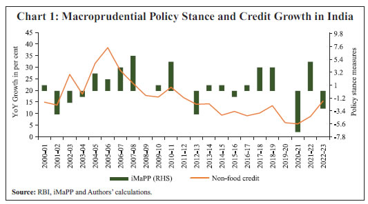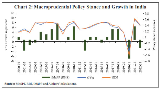

Section IV
Empirical Framework

As discussed earlier, the empirical framework uses the growth-at-risk approach. First, the effect of policy stance is analysed on the tails of non-food credit growth distribution. Next, a similar analysis is used for output gap to evaluate the policy effects on the tails of the output gap distribution. Lastly, credit growth is linked to the output gap distribution by looking at the average effects during high and low credit growth phases. The causality between macroprudential policy with output is evaluated at the tails by linking the credit effect with the tail effects on output gap.

To estimate the tail effects of macroprudential policies on credit growth and output gap, quantile regression approach is adopted. Since the macroprudential policies work with lags, the policy effect has been estimated using local projection approach, as suggested by Jorda (2005).

Section V
Empirical Findings

In the first leg, the effect of macroprudential policy on credit growth is evaluated across quantiles. These effects are presented along with their confidence bands, derived using the bootstrapped standard errors. When credit growth is very high i.e., the credit growth is at 90th percentile, tighter macroprudential policy reduces the credit growth over the medium horizon. On the other hand, the effect is not highly significant when credit growth is low (Chart 3)⁶.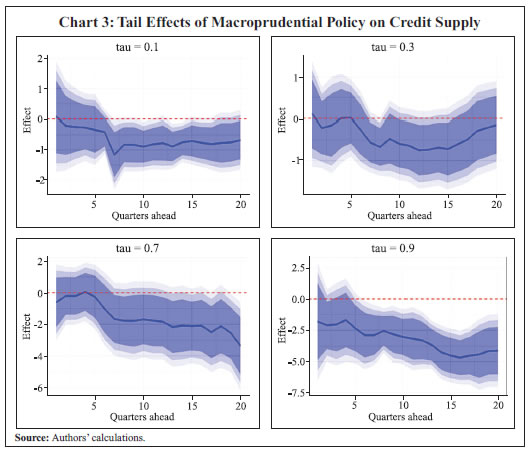

The policy effect is then evaluated on the distribution of the output gap over different time horizons. Tight macroprudential policy supports output when the output gap is highly negative⁷, whereas when the output gap is highly positive, it turns out to be insignificant. When the output gap is highly negative, the macroprudential policy helps in narrowing the negative output gap. The effect is significant at the 10th and 30th percentiles. On the other hand, macroprudential policy does not significantly impact output at the upper tails. This implies that the cost of implementing a tight macroprudential policy is outweighed by its benefits when the output gap is positive i.e., the economy is operating above its potential level (Chart 4). Similar findings are obtained using GDP growth rates (see Chart A1.2 in Annex 1 and Chart A3.2 in Annex 3). When the economy is in slack, the relaxation in macroprudential policy helps in improving output growth by facilitating better credit supply. This aligns with the countercyclical nature of the macroprudential policies.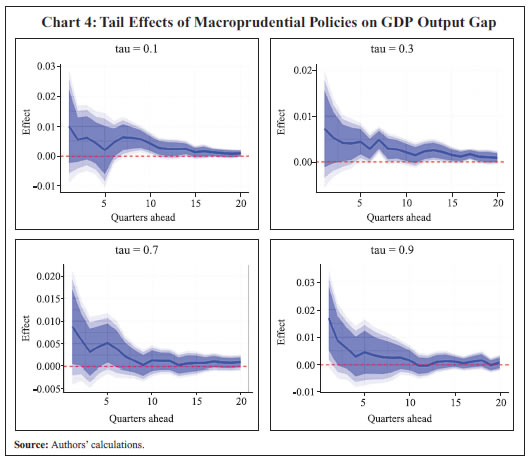

The macroprudential policy is generally addressed to reduce systemic risks and these measures reduce default risks and strengthen banks’ asset quality and health ensuring adequate credit supply across economic cycles (coefficient estimates provided in Annex 2).

A similar effect is visible on the output gap measured using GVA. The lower tail effect of a tighter policy is even more prominently visible in this case. Further, the effect remains statistically significant over a 3-4 year horizon. Here too, the upper tail effect remains insignificant. The findings are similar in case of output gap measured using non-agriculture GVA (NAGVA) (Charts 5 and 6).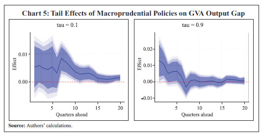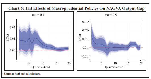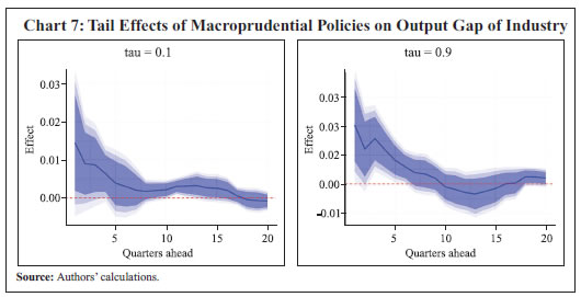

Further, the positive effect of the macroprudential policy on NAGVA is drilled down to check the tail effects on industry and services⁸. Using the same empirical framework on the output gap of industry and services, the findings highlight a positive effect of the macroprudential policy on the average output gap of industry and services at the lower tail. The effect is more prominent for services than industries (Charts 7 and 8).

Next, the tail effects of macroprudential policies are checked on PFCE and investment cycles. Like GDP growth and output gap, the tighter policy effects are visible in consumption cycles when the consumption is growing at a slower pace (i.e., when the consumer growth is in the 10th percentile of its distribution). The upper tail (i.e., when the consumer growth is in the 90th percentile of its distribution) effects are statistically insignificant (Chart 9).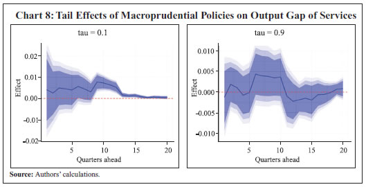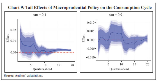

The lower tail effect of tighter policies improves investment over the medium term, but the effect is weakly significant. The upper tail effect is statistically insignificant (Chart 10).

The analysis suggests that credit growth moderates in response to a restrictive macroprudential policy shock when it is already high. On the other hand, the effects of the macroprudential policy on the lower tail of the output gap i.e., when the output gap is highly negative, highlight benefits which outweigh the short-term costs of implementing these policies. In the last leg of empirical validations, the effect of credit growth on output gap is evaluated over the distribution of the output gap.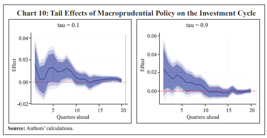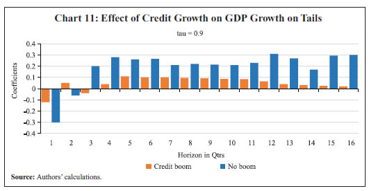

When the output gap is highly negative, credit supply facilitates economic growth over the short and medium-term horizons i.e., higher credit growth facilitates faster recovery when the economic activity is below its potential. The marginal effects are more pronounced when credit growth is low. On the upper tail, i.e., when the output gap is already at a higher level, the additional credit supply improves output only marginally. The effect is higher if the existing credit growth is low. Higher credit growth in such circumstances facilitates greater investments and fuels economic growth. However, if the credit growth is already at a high level, then the additional credit does not translate into higher growth (Chart 11).

We employ a number of robustness checks. As the study period covers the COVID-19 pandemic, which may contaminate the results, we attempt an estimation excluding the pandemic period. The estimates show similar effects (Charts A1.1 and A1.2 for the tail effects on credit growth and output gap, respectively, in Annex 1). Further, the estimation is carried out using year-on- year (YoY) growth rates of credit, GDP, PFCE and GFCF for full sample as well as for pre-COVID-19 period. The results are again on similar lines (Annex 3).

Section VI
Conclusion

The macroprudential policy measures play an important role in fostering financial stability. However, the short-term cost of implementing these policies often leads to debates about their net benefits. In this context, this paper assessed the effects of macroprudential policies on the distribution of credit and output over different horizons using a quantile regression approach in a local projection framework.

The empirical analysis suggests that tighter macroprudential policies help in containing credit growth when the credit growth is already high; the effect persists in the medium to long term. The normalisation of macroprudential policies from their earlier restrictive state improves output by narrowing the negative output gap at the time of economic slackness. However, the effect is statistically insignificant when output growth is highly positive. Using different measures of the output gap, we observe similar effects. We observe statistically significant favorable effects of normalisation of macroprudential policies especially on the services sector when it is performing below its potential. A tighter policy stance ensures financial stability by moderating credit growth, facilitating higher output over the medium term. Overall, the benefits of the macroprudential policy outweigh its costs.

References

Adrian, T., de Fontnouvelle, P., Yang, E., & Zlate, A. (2017). Macroprudential policy: A case study from a tabletop exercise. Economic Policy Review, 23-1, 1-30.

Adrian, T., Boyarchenko, N., & Giannone, D. (2019). Vulnerable growth. American Economic Review, 109(4), 1263-1289.

Adrian, T., Grinberg, F., Liang, N., Malik, S., & Yu, J. (2022). The term structure of growth-at-risk. American Economic Journal: Macroeconomics, 14(3), 283-323.

Aikman, D., Bridges, J., Hoke, S. H., O’Neill, C., & Raja, A. (2019). How do financial vulnerabilities and bank resilience affect medium-term macroeconomic tail risk. Bank of England Working Paper. 824.

Akinci, O., & Olmstead-Rumsey, J. (2018). How effective are macroprudential policies? An empirical investigation. Journal of Financial Intermediation, 33, 33-57.

Alam, Z., Alter, M.A., Eiseman, J., Gelos, M.R., Kang, M.H., Narita, M.M. & Wang, N. (2019). Digging deeper–evidence on the effects of macroprudential policy from a new database. International Monetary Fund.

Abbate, A. & Thaler, D. (2019). Monetary policy and the asset risk-taking channel. Journal of Money, Credit and Banking. 51, 2115-2144.

Angeloni, I., & Faia, E. (2013). Capital regulation and monetary policy with fragile banks. Journal of Monetary Economics. 60(3), 311-324.

Banu, I. M. (2013). The impact of credit on economic growth in the global crisis context. Procedia Economics and Finance. 6, 25-30.

Belkhir, M., Naceur, S.B., Candelon, B., Wijnandts, J. (2020). Macroprudential policies, economic growth, and banking crises, IMF Working Paper. 2020/065.

Boar, C., Gambacorta, L., Lombardo, G. & Pereira da Silva, L. A. (2017). What are the effects of macroprudential policies on macroeconomic performance? BIS Quarterly Review. September, 71-88.

Buch, C., Vogel, E., & Weigert, B. (2018). Evaluating macroprudential policies. Working Paper Series, European Systemic Risk Board. 76.

Carrasquilla , A., Arturo G. A., Vásquez, D.M. (2000). El gran apretón crediticio en Colombia: una interpretación, Coyuntura Económica, Fedesarrollo, March.

Cartapanis, A. (2011). Financial crisis and macro-prudential policies. Revue economique, 62(3), 349-382.

Cerutti, E., Claessens, S., & Laeven, L. (2015). The use and effectiveness of macroprudential policies: New evidence. IMF Working Paper. 15/61.

Chakrabarty, K. C. (2014). Framework for the conduct of macroprudential policy in India: experiences and perspectives. Financial Stability Review, Banque de France. 18, 131-144.

Claessens, S. (2015). An overview of macroprudential policy tools. Annual Review of Financial Economics. 7, 397-422.

Collin, M., Druant, M., & Ferrari, S. (2014). Macroprudential policy in the banking sector: Framework and instruments. Financial Stability Review, National Bank of Belgium. 12(1), 85-97.

Dell’Ariccia, G., Laeven, L., & Suarez, G. A. (2013). Bank leverage and monetary policy’s risk‐taking channel: Evidence from the United States. IMF Working Paper. 13/143.

Fernandez-Gallardo, A. (2023). Preventing financial disasters: Macroprudential policy and financial crises. European Economic Review. 151, 104350.

Franta, M., & Gambacorta, L. (2020). On the effects of macroprudential policies on growth-at-risk. Economics Letters. 196, 109501.

Galán, J. E. (2020). The benefits are at the tail: Uncovering the impact of macroprudential policy on growth-at-risk. Journal of Financial Stability,100831.

Galati, G. & Moessner, R. (2013). Macroprudential policy – A literature review. Journal of Economic Surveys. 27, 846-878.

Galati, G. & Moessner, R. (2018). What do we know about the effects of macroprudential policy? Economica. 85, 735-770.

Hung, F. S., & Cothren, R. (2002). Credit market development and economic growth. Journal of Economics and Business. 54(2), 219-237.

IMF (2013). The Key Aspects of Macroprudential Policy: IMF Policy Paper. International Monetary Fund. June.

Jordà, Ò. (2005). Estimation and inference of impulse responses by local projections. American Economic Review. 95(1), 161-182.

Kim, S. (2019). Macroprudential policy in Asian economies. ADB Economics Working Paper Series. 577.

Kumar, S., Prabheesh, K. P., & Bashar, O. (2022). Examining the effectiveness of macroprudential policy in India. Economic Analysis and Policy. 75, 91-113.

Kuttner, K. N. & Shim, I. (2016). Can non-interest rate policies stabilize housing markets? Evidence from a panel of 57 economies, Journal of Financial Stability. 26, 31-44.

Lim, C., Columba, F., Costa, A., Kongsamut, P., Otani, A., Saiyid, M., Wezel, T. & Wu, X. (2010). Macroprudential policy: What instruments and how to use them? IMF Working paper. 11/238.

Lloyd, S., Manuel, E., & Panchev, K. (2024). Foreign vulnerabilities, domestic risks: The global drivers of GDP-at-risk. IMF Economic Review. 72, 335–392.

Ma, C. (2020). Financial stability, growth and macroprudential policy. Journal of International Economics. 122, 103259.

Meuleman, E., & Vennet, R. V. (2020). Macroprudential policy and bank systemic risk. Journal of Financial Stability, 47, 100724.

Milne, A. (2009). Macroprudential policy: What can it achieve? Oxford Review of Economic Policy, 25(4), 608-629.

Peydró, J. L. (2016). Macroprudential policy and credit supply. Swiss Journal of Economics Statistics, 152, 305-318.

Reinhart, C. M., & Rogoff, K. S. (2009). The aftermath of financial crises. American Economic Review. 99 (2), 466-72.

Richter, B., Schularick, M., & Shim, I. (2019). The costs of macroprudential policy. Journal of International Economics. 118, 263-282.

Saraf, R., & Chavan, P. (2023). Sectoral efficacy of macroprudential policies in India. Economic and Political Weekly. 58(21), 51-60.

Sassi, S. (2014). Credit markets development and economic growth: Theory and evidence. Theoretical Economics Letters. 4(9), 767-776.

Singh, C., Pemmaraju, S. B., & Das, R. (2018). Economic growth and credit in India. International Review of Business and Economics. 1(2), 10.

Sinha, A. (2011). Macroprudential policies-Indian experience. Speech delivered at the 11th Annual International Seminar on Policy Challenges for the Financial Sector on “Seeing both the Forest and the Trees-Supervising Systemic Risk,” Washington D.C.

Unsal, D.F., (2013). Capital flows and financial stability: monetary policy and macroprudential responses. International Journal of Central Banking. March, 234-285.

Vandenbussche, J., Vogel, U., & Detragiache, E. (2015). Macroprudential policies and housing prices: A new database and empirical evidence for Central, Eastern, and Southeastern Europe. Journal of Money, Credit and Banking. 47, 343-377.

Verma, R. (2018). Effectiveness of macroprudential policies in India. Macroprudential Policies in SEACEN Economies. 31-54.

Zhang, Y., & Tressel, T. (2017). Effectiveness and channels of macroprudential policies: Lessons from the Euro area. Journal of Financial Regulation and Compliance. 25(3), 271-306.

Annex 1: Pre-COVID-19 Period Estimates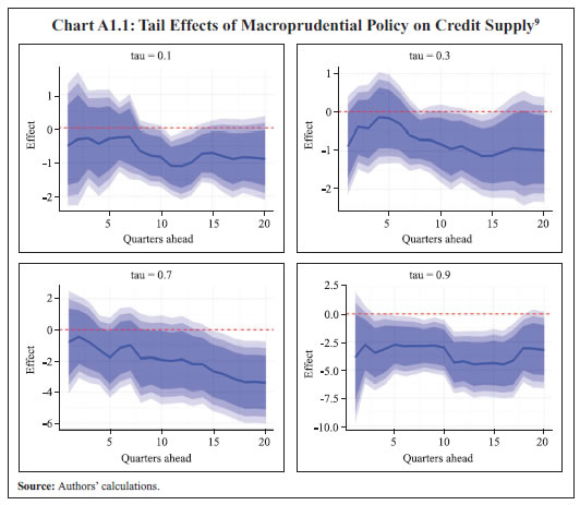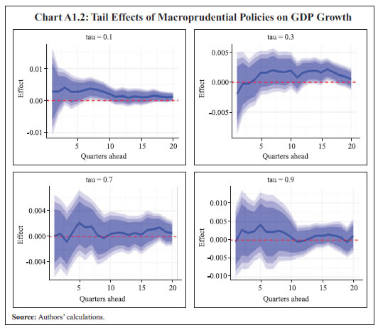

Annex 3: Tail Effects of Macroprudential Policies on YoY Growth Rates (Full Sample)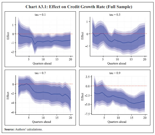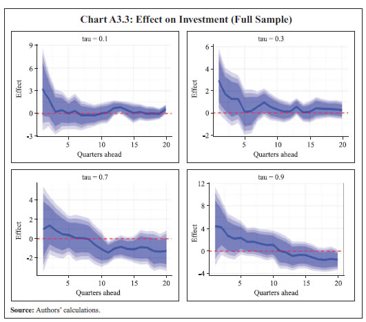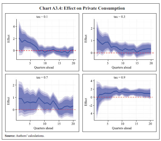

^* The authors are Assistant Adviser (asanyal@rbi.org.in) and Director, respectively, in the Department of Statistics and Information Management, Reserve Bank of India. They are thankful to Rakesh Kumar and other seminar participants at the DEPR Study Circle, and an anonymous referee for their comments/suggestions. The views expressed in this paper are those of the authors and not of the organisation to which they belong.

¹ The policy stances were classified on a three-point scale to synergise with the iMaPP data compiled by IMF.

² These policy actions are considered in the iMaPP database, though some of these were not applied in India.

³ The new base for the GDP series starts from 2011 onwards at a quarterly frequency. The older data are available at an annual frequency. The quarterly back series is constructed by applying quarterly shares from previous base estimates (2004-05) on the annual back series published by MoSPI. The bank credit data and non-food credit data are sourced from RBI.

⁴ For robustness, the WPI headline index is also used as a deflator. The results are found to be similar.

⁵ Output gap is measured as deviation from the potential output using the HP filter.

⁶ The shaded regions in Charts 3 to 10 represent confidence band at 90 per cent (dark blue), 95 per cent (lighter blue) and 99 per cent (lightest blue).

⁷ The lower quantiles of output gap correspond to large negative output gap.

⁸ The tail effect on agriculture is not considered in this analysis. This is because agricultural activities in India are primarily driven by rainfall and weather conditions.

⁹ The shaded regions in Charts A1.1 to A1. 2 and in Annex 3 represent confidence band at 90 per cent (dark blue), 95 per cent (lighter blue) and 99 per cent (lightest blue).