 IST,
IST,


Measuring Productivity at the Industry Level - The India KLEMS Database
|
AUTHORS Sadhan Kumar Chattopadhyay Director Siddhartha Nath Assistant Adviser Sreerupa Sengupta Manager Shruti Joshi Manager
This document describes the procedures, methodologies and approaches used in constructing the India KLEMS database version 2021. Till now, the work relating to compilation of India KLEMS data was being done by the India KLEMS team housed at the Centre for Development Economics, Delhi School of Economics. Now the work has been shifted to the KLEMS Division of Department of Economics and Policy Research of RBI since February 2021 and hence the KLEMS data have been compiled independently by the KLEMS Division under the supervision of India KLEMS team. This work is meant to support empirical research in the area of economic growth. In addition, the database is meant to support the conduct of policies aimed at supporting acceleration of productivity growth in the Indian economy, requiring comprehensive measurement tools to monitor and evaluate progress. Finally, the construction of the database would also support the systematic production of reliable statistics on growth and productivity using the methodologies of national accounts and input-output analysis. Following the earlier trend, this version of database includes measures of economic growth, employment creation, capital formation and productivity at the industry level from 1980-81 onwards. The input measures will incorporate various categories of Capital (K), Labour (L), Energy (E), Materials (M) and Services (S) inputs. The present document describes the India KLEMS database version 2021. In fact, the present version is an extended India KLEMS research project, “Disaggregate Industry Level Productivity Analysis for India- the KLEMS Approach” undertaken at the Centre for Development Economics, Delhi School of Economics. The dataset includes measures of Gross Value Added (GVA), Gross Value of Output (GVO), Labour (L), Capital (K), Energy (E), Material (M), Services (S), Labour Quality (LQ), Labour Productivity (LP) and Total Factor Productivity (TFP) at the industry and economy level from 1980-81 onwards. The database covering the period 1980-81 to 2019-20 has been constructed on the basis of data compiled from NSO, NSSO, ASI, Input-Output tables (I-O tables) and processed according to appropriate procedures. These procedures were developed to ensure harmonization of the basic data, and to generate growth accounts in a consistent and uniform way. Harmonization of the basic data has focused on several areas such as industrial classification, and aggregation levels. The data base covers 27 industries comprising the entire Indian economy. The industries are shown in Table 1.1 below. The variables in the data set are given in Table 1.2. 1.2 Coverage: Industries and Variables In this section we describe the coverage of the India KLEMS database in terms of industries and variables. In principle, the 39-year period from 1980-81 (1980) to 2019-20 (2019) is covered. At a disaggregated level, database is created for 27 industries. The industrial classification is constructed by building concordance between NIC 2008, NIC 2004, NIC 1998, NIC 1987 and NIC 1970 to generate continuous time series from 1980 to 2019. This classification is very close to the International Standard Industrial Classification (ISIC) revision 3. The 27 industries are aggregated to form six broad sectors, namely:
Table 1.1 provides a listing of the 27 industries, including the higher aggregates. For detailed classification and concordance of study industries with NICs, readers may refer to Version 7 of the manual published in 2021. Table 1.2 provides an overview of all the series included in our database. Measures of Capital (K), Labour (L), Energy (E), Material (M) and Service (S) inputs as well as Gross Output (GO), have been constructed using National Accounts Statistics (NAS), Annual Survey of Industries (ASI), NSSO rounds and Input-Output (IO) Tables. In building annual time series on gross output, five inputs and factor income shares, various assumptions are made to fill up gaps in industry details and link series over time. As we know that NSSO rounds of unregistered manufacturing, Input Output Transaction Tables, and Employment and Unemployment Surveys by NSSO are available only for certain benchmark years. The use of information from these data sources necessitates interpolation and assumption of constant shares for building series of output and inputs. Further the construction of growth accounting series like total factor productivity, labour productivity, etc. are based on theoretical models of production and needs additional assumptions that are spelt out in subsequent chapters of the manual. Finally, the other Series like NDP at factor cost, compensation of employees, etc. are additional series which are used in generating the growth accounts and are informative by themselves. Chapter 2: Gross Value-Added Series at the Industry Level This chapter describes the data sources and methodology used to construct the Gross Value Added (GVA) series at current and constant prices for 27 study industries for the period of 1980-81 (1980) to 2019-20 (2019). The National Accounts Statistics (NAS) brought out by the NSO (National Statistics Office, Government of India) is the basic source of data for the construction of series on gross value added for INDIA KLEMS-industries. Up to 2011-12, estimates of GVA at both current and constant (2011-12) prices for all industries are obtained from Back Series of National Accounts (Base 2011-12). For years after 2011-12, they are directly obtained from NAS 2022. However, NAS estimates of value added are not available for a few India KLEMS industry groups. Therefore, we had to split some of the aggregate industry groups from NAS. Maintaining consistency with NAS, the value-added data in India KLEMS is measured at basic price. The construction of Gross valued added series involves three steps. Step 1: A concordance table between the classification used in the NAS and the 27 study industry classification used for this project has been prepared. Further, concordance between all the 27 sectors has been constructed with NIC- 1970, 1987, 1998, 2004 and 2008. Out of the 27 study industries, for 20 industries, GVA series both in current and constant prices is directly taken from NAS1. The sectors for which data are provided in NAS are Agriculture, Forestry & logging, Fishing, Mining and Quarrying, Manufacturing, Electricity,gas and water supply, Construction, Trade, Hotels & Restaurants, Railways, Transport by other means, Storage, Communication, Banking & insurance, Real estate, Ownership of Dwelling & Business Services, Public Administration & Defense and Other Services. Step 2: For manufacturing industries where direct estimates of GVA were not available from NAS, estimates have been made using additional information from ASI and NSSO unorganized manufacturing data. In these cases, GVA data is constructed by splitting the NAS data using ASI or NSSO distributions. ASI data (annual) has been used for registered and corporate manufacturing whereas interpolated ratios from NSSO 40th (1984-85), 45th (1989-90), 51st (1994-95), 56th (2000-01) 62nd (2005-06), 67th round (2010-11) and 73rd round (2015-16) rounds have been used for Unregistered and household manufacturing segments. For unregistered manufacturing for years 2015-16 to 2019-20 the ratio obtained from 73rd round of unregistered manufacturing has been used for the splitting. Table 2.1 and 2.2 showcases the methodology used to split GVA of certain NAS sectors to match concordance with our classification. It is important to note that the industry level value added volume indices are based on NAS. NSO provides single deflated value-added estimates for all sectors except Agriculture. Step 3: According to India KLEMS, GVA is adjusted for Financial Intermediation Services Indirectly Measured (FISIM). The details method of FISM adjustment is provided in earlier versions of KLEMS manual. Chapter 3: Gross Output Series at the Industry Level This chapter describes the procedures and methodologies used in constructing the database for gross output series at the industry level over the period 1980-81(1980) to 2019-20(2019). To construct the gross output series at industry level, we use multiple data sources namely National Accounts Statistics, Annual Survey of Industries, NSSO rounds for unorganized manufacturing and Input Output Transaction tables. The data sources and methodology used are documented below: National Accounts Statistics: The NAS is the basic source of data for the construction of time series on the gross output. The NAS back series 2011 with base 2004-05 and NAS 2014 provides estimates of gross output for six disaggregate industries at current and constant prices since 1950-51 till 2011-12. These sectors are Agriculture, Mining and Quarrying, Construction and Manufacturing sectors (Registered and Unregistered Manufacturing). However, the Back Series with base 2011-12, which is the source of GVA in India KLEMS database 2021, does not provide estimates of GVO for most of the industries except for Agriculture, Mining and Quarrying and Construction. For these three industries GVO data at current and constant prices directly obtained from Back Series with base 2011-12. Therefore, for 1980-81 to 2011-12 period, we estimate the GVO series for remaining 24 industries at current and constant prices by applying the respective GVO/GVA ratio for current and constant prices obtained from Back Series with base 2004-05 and NAS 2014 to GVA with 2011-12 base. For years since 2011, we take the estimates of GVO both at current and constant prices for all industries directly from NAS 2022. (a) Filling procedures of National Accounts series: It is to be noted that the NAS estimates of gross output for a few industry groups are at a more aggregate level, requiring splitting of the aggregates. In such cases, NAS estimates of output have been split using additional information from Annual Survey of Industries and NSSO rounds of Unregistered Manufacturing to obtain estimates at higher level of disaggregation. Secondly, for Unregistered manufacturing gross output data is available in NAS from 2004-05 onwards. In this case, information from NSSO survey rounds has been used for missing years to derive output estimates of unregistered manufacturing industries at current and constant prices. As mentioned earlier, for gross value-added series of service sectors we obtain our estimates from NAS. However, prior to 2011-12 National Accounts do not provide any estimates of gross output of service sectors and hence we rely on Input output transaction tables (from which the ratio of gross to value added is computed which is then applied to GVA reported in NAS) which are available at an interval of 5 years or so. This necessitates interpolation and assumption of constant shares for measuring output of services sectors. The Input Output Transaction Tables for Benchmark years of 1978-79, 1983-84, 1989-90, 1993-94, 1998-99, 2003-04 and 2007-08 are used to derive gross output series for service sectors. The construction of the gross output series at current and constant prices involves the following steps: Step 1: Measuring Gross Output of Agricultural Sector, Mining and Quarrying, and Construction NAS provides nominal and real GVO series for a) Crops and Plantation, b) Animal Husbandry c) Forestry and Logging d) Fishing. By aggregating the GVO of these four subsectors we derive the GVO of Agricultural sector. The Gross output estimates of Mining and Quarrying and Construction at current and constant prices from 1980-2019 is also directly taken from NAS. Step 2: Measuring Gross Output of Manufacturing Industries Since 2011-12, gross output data for 7 out of 13 manufacturing industries listed in table 3.1 are directly picked up from NAS. For the remaining 6 sectors output is constructed by splitting the NAS output data using ASI or NSSO distributions. ASI data (annual) has been used for registered manufacturing whereas interpolated ratios from 67th (2010-11) and 73rd (2015-16) rounds have been used for Unregistered Manufacturing segments. A list of study industries is presented in Table 3.2 showcasing the methodology used to split GVO of certain NAS sectors to match concordance with our classification for the year 2011 to 2019. Step 3: Measuring Gross Output for Services Sectors and Electricity, Gas and water supply Since 2011-12 NAS provided estimates of GVO at current and constant prices. Prior to 2011-12 Gross Output series for Services sectors and sector Electricity, Gas and Water supply have been constructed using information from Input – Output Transaction Tables of the Indian economy published by CSO. The details method of construction of GVO back series for services is provided in earlier versions of KLEMS Data manual. Chapter 4: Labour Input Series at the Industry Level This chapter provides information on the sources of data and method of measuring labour services. The aim is to estimate labour input so that it reflects the actual changes in the quantity (number of persons) and quality of labour input over time. The section discusses the construction of labour input for 27 industries from 1980 to 2019-20. Labour input is measured by combining data on labour persons and data on labour quality which is measured in terms of human capital embodied in the labour. In our study, we measure this on the basis of the educational qualification of the worker. It is important to segregate labor employed from labor quality because the contribution to output by each person also comes from this embodied capital. Moreover, the reward (wages and earnings) to each person also includes the reward for investment in human capital. Therefore, it is essential to separate out these differences in labour to clearly understand the underlying differences in labour characteristics. It is in this context that an endeavor has been made to estimate labour quality index. However, given the limitations of India’s employment statistics (Sivasubramonian; 2004, & Himanshu; 2011, Ghose; 2016), especially the availability of information on wages/ earnings of different category of workers which could be used as an indication of their differences in ability makes it difficult to quantify these changes in the labour force in a pertinent way. Therefore, the study has computed the labour quality index based on five different education categories only. This study aims to build a time series of employment and labor quality series for 27 industrial sectors. In this section we outline the sources of data and the methodology used. The section develops and implements the methodology of estimating persons employed (employment) and labour quality and combining the two to obtain the indices of labour input. Sources of data The Employment and Unemployment Surveys (EUS) of major rounds from 38th round (1983) to 68th round (2011-12) by National Sample Survey Office (NSSO) and the Periodic Labour Force Surveys (PLFS) of 2017-18, 2018-19 and 2019-20 by National Statistical Organization (NSO) are the main sources for estimating the total workforce in the country by industry groups, as per the National Industrial Classification (NIC). This year the study has adjusted the employment estimates obtained from Economic-Survey 2021-22 (pp.371). Methodology The employment in India has been computed in a step-wise manner as follows: As a first step concordance between the KLEMS 27 sectors, and NIC-1970, 1987, 1998 and 2008 was done. Thereafter, the following steps were done:
For extrapolation backward to 1980-81 to 1982-83, the interpolation of the broad industrial classification of 32nd round (1977-78) and 38th round (1983-84) is used. Thus, the estimates from 32nd round are mainly used as control numbers. Between 2005 and 2011, we observed very high growth rate in number of employed persons series for the industry Electrical and Optical Equipment as compared to other manufacturing industries and the overall growth in employment in this industry during 2005-2011 was found to be higher than that for Construction (which seems somewhat unrealistic). It was also observed that there was a negative growth in employment in Textiles, Textile Products, Leather and Footwear although real GVA of this industry more than doubled between 2005 and 2011. To address these issues, some adjustments to the initial employment estimates for Electrical & Optical Equipment and Textiles, Textile Products, Leather and Footwear have been done. Onwards 2005, employment series for Electrical & Optical Equipment has been estimated applying annual growth rates obtained from ASI and NSSO rounds to the number of employed persons for the year 2005-06. Then, for the years 2005-06 to 2011-12, we compute the difference between estimated employment series from EUS rounds and that based on ASI & NSSO rounds for the Electrical and Optical Equipment industry and add it to Textiles, Textile Products, Leather and Footwear industry. This ensures that for the manufacturing as a whole our estimates remain the same as obtained from EUS rounds. (b) Measuring quality index The quality of labour force is of considerable importance in the context of productivity measurement, and one of the widely used methodologies to capture changes in labour quality is given by Jorgenson, Gollop and Fraumeni (JGF) (1987). In growth accounting methodology of measurement of total factor productivity (TFP) when output growth is decomposed into growth of inputs and the residual TFP, then labour input is measured as an index of labour service flows. It accounts for changes in labour quality in terms of labour characteristics such as educational attainment, age (experience), gender, employment status, etc. and thus accounts for heterogeneity of the labour force. In our study, the index of aggregate labour quality measures the changes in the composition of labour in the economy. The present study has computed labour quality index by using only education characteristic in the JGF methodology. Thus, the data required for the labour quality index in the present case, is employment and earnings by education and by industry. The labour quality index has been computed using five education categories namely- up to primary, primary, middle, secondary & higher secondary, and above higher secondary. There are thus five types of persons employed for each of the 27 study industries. The quality growth rates are estimated for total persons employed in these industries in India for the 38th, 50th, 55th, 61st, 68th and PLFS rounds of NSO. They are then indexed to 1983 (38th round) as the base, so as to assess the temporal changes in labour’s skill and interpolation has been done between the major rounds for values of the intermediate years. Since the series is required from 1980-81, we have extrapolated it backwards from 1983 and the index is recomputed with base 1980-81 equal to 100. Therefore, the following steps have been performed:
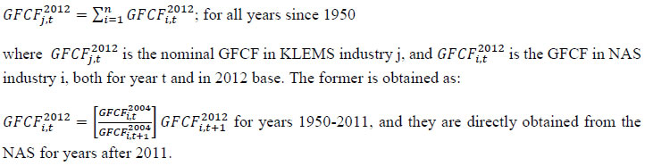
 The first term of equation 4.1 indicates the changes in labour quality index, which is due to the changes in the composition of workers and the second term indicates the change in total persons employed in sector ‘j’. The index of aggregate labour quality thus measures the changes in the composition of labour in the economy The labour input (adjusted labour persons) then can be obtained by multiplying the number of persons employed by the corresponding labour quality index and the labour input growth is finally obtained by combining the growth of persons employed and the growth in the index of labour quality. Appendix A: Definitions of Employment in NSSO employment & unemployment surveys The surveys of NSSO on employment and unemployment (EUS) aim to measure the extent of ‘employment’ and ‘unemployment’ in quantitative terms disaggregated by various household and population characteristics following the three reference periods of (i) one year, (ii) one week, and (iii) each day of the week. Based on these three reference periods three different measures, termed as usual status, current weekly status, and the current daily status, are arrived at. While all these three approaches are used for collection of data on employment and unemployment in the quinquennial surveys, the first two approaches only are used for the purpose in the annual surveys. Usual principal status: In NSS 27th round, the usual principal activity category of the persons was determined by considering the normal working pattern, i.e., the activity pursued by them over a long period in the past and which was likely to continue in the future. For the identification of the usual principal status of an individual based on the major time criterion, in NSS 27th, 32nd, 38th, 43rd rounds, a trichotomous classification of the population was followed, that is, a person was classified into one of the three broad groups ‘employed’, ‘unemployed’ and ‘out of labour force’ based on the major time criterion. From NSS 50th round onwards, the procedure was changed and the prescribed procedure was a two-stage dichotomous one which involved a classification into ‘labour force’ and ‘out labour force’ in the first stage, and thereafter, the labour force into ‘employed’ and ‘unemployed’ in the second stage. Usual subsidiary status: In the usual status approach, besides principal status, information in respect of subsidiary economic status of an individual was collected in all employment and unemployment surveys. For deciding the subsidiary economic status of an individual, no minimum number of days of work during the last 365 days was mentioned prior to NSS 61st round. In NSS 61st round, a minimum of 30 days of work, among other things, during the last 365 days, was considered necessary for classification as usual subsidiary economic activity of an individual. Current weekly status: It is important to note at the beginning that in the EUS of NSSO, a person is considered as worker if he/she has performed any economic activity at least for one hour on any day of the reference week and uses the priority criteria in assigning work activity status. This definition is consistent with the ILO convention and used by most of the countries in the world for their labour force surveys. In NSSO, prior to NSS 50th round and in all the annual surveys till NSS 59th round, data on employment and unemployment in the CWS approach was collected by putting a single-shot question ‘whether worked for at least one hour on any day during the last 7 days preceding the date of survey’. The information so collected was used to determine the CWS of the individuals. This procedure was criticized for being not able to identify the entire workforce, particularly among the women. It was then decided to derive the CWS of a person from the time disposition of the household members for the 7 days preceding the date of survey. The procedure was used for the first time in NSS 50th round. It is seen that the change in the method of determining the current weekly activity had resulted in increasing the WPR in current weekly status approach - more so for the females in both rural and urban areas than for males. The trend observed in NSS 50th round in respect of the WPR according to CWS suggested continuing with the procedure for data collection in CWS in NSS 55th and NSS 61st rounds. Current Daily Status Current Daily Status (CDS) rates are used for studying intensity of work. These are computed on the basis of the information on employment and unemployment recorded for the 14 half days of the reference week. The employment statuses during the seven days are recorded in terms of half or full intensities. An hour or more but less than four hours is taken as half intensity and four hours or more is taken as full intensity. An advantage of this approach was that it was based on more complete information; it embodied the time utilisation, and did not accord priority to labour force over outside the labour force or work over unemployment, except in marginal cases. A disadvantage was that it related to person-days, not persons. Hence it had to be used with some caution. Chapter 5: Capital Input Series at the Industry Level This chapter outlines the methodology employed to estimate capital input for the 27 industries in the India KLEMS database version 2022. All the productivity calculations in India KLEMS use capital services as an input to production, which is estimated using the approach developed by Jorgenson and Griliches (1967), and outlined in Jorgenson, Gollop, and Fraumeni (1987). The estimation of capital service growth rates is accomplished by first estimating capital stock for different capital assets, and then aggregating across assets after correcting for the differences in their marginal productivities. Capital services account for the differences in marginal productivity between different asset types while capital stock measures only the vintages of capital, they do not account for asset heterogeneity. For instance, aggregate capital stock measures would assume that a computer's productivity is the same as that of a car. However, proper measures of capital stock would account for the decline in the efficiency of both computers and cars over their lifetime. Following an overview of the theoretical method to measure capital services (Jorgenson and Griliches,1967; JGF, 1987), the chapter discusses the specific empirical approaches we follow to implement these methods within the constraints of data availability for Indian industries. In India KLEMS, we have reported capital stock, capital services and the capital “capital composition effect”. Capital stock is reported in constant price volumes, and growth rates, while the latter two are reported in growth rates and indices. To measure capital services, using the Jorgenson and Griliches (1967) approach, we need estimates of capital stock for detailed asset types and the shares of each of these assets in total capital remuneration. The aggregate capital services growth rate is derived as a weighted growth rate of individual capital assets, the weights being the shares of each asset in the total compensation made to capital, i.e, 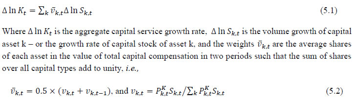 where PKk,t is the rental or user cost of capital asset type k in year t. Therefore, the numerator, which is the product of user cost of asset k and the capital stock of asset k, is the capital compensation received by asset k. The numerator is the sum of compensation received by assets, or the total capital compensation, and therefore vk,t is the share of asset k in total capital compensation. Under the neoclassical assumption of price-marginal product equality, it effectively incorporates the productivity or qualitative differences in the contribution of various asset types to aggregate capital services, as the composition of aggregate capital stock in any industry changes (see Jorgenson, 2001). For instance, as the marginal productivity of ICT capital is higher than that of other assets, a change in the composition of capital towards ICT capital will result in higher capital services, which will be captured by a larger value of the v for ICT assets. It is evident from (5.2) that two important components of capital service measure are the asset wise capital stock, Sk,t and the service price (rental price) of capital assets, PKk,t. Assuming a geometric depreciation rate, δk which is constant over time, but different for each asset type, capital stock in asset k in year t can be constructed using Perpetual Inventory Method (PIM) as:7  where, Ik,t is the real investment in asset type k in period t. For a detail discussion on PKk,t, please see Box 5.1A in the Appendix B. 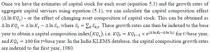 Since our measure of capital input takes account of asset heterogeneity, it was essential to obtain investment data by asset type. We distinguish between 3 different asset types – construction, transport equipment, and machinery (includes ICT and non-ICT machinery).8 We exploit multiple sources of information for the construction of our database on capital services. This includes the National Accounts Statistics (NAS) that provide information on broad sectors of the economy, the Annual Survey of Industries (ASI) covering the organized manufacturing sector, the National Sample Survey Office (NSSO) rounds for unorganized manufacturing and various Input-Output tables. Even though we use multiple sources of data, our final estimates are fully consistent with the aggregate data obtained from the NAS. In addition, our approach to capital measurement is consistent with international practices such as the EU KLEMS9, which ensures the possibility of international comparisons. In what follows, we discuss the various sources of data for asset wise investment and the construction of the relevant variables, in detail. (a) Asset-wise investment for broad sectors of the economy Industry-level estimates of capital input require detailed asset-by-industry investment matrices. NAS provides information on aggregate capital formation by industry of use for nine broad sectors, which, nevertheless, was not sufficient for our purpose. Therefore, we have collected more detailed data on assets and industries from the CSO.10 This is the data underlying the published aggregate gross fixed capital formation by the broad industry groups, separately for public and private sectors. For those sectors for which the investment matrices were not available from CSO, we gather information from other sources (e.g. ASI for organized manufacturing and NSSO surveys for unorganized manufacturing) and benchmark it to the aggregate investment series from the National Accounts. The data used in the current version of the India KLEMS is based on the revised NAS with 2011-2012 base and is available only since 2012. Therefore, for earlier years, we extrapolate the series using growth rates from previous version of the data. Table 5.1 provides an overview of asset types available in NAS and their corresponding asset types used in our study. Investment in education and health are obtained directly from national accounts for the period after 2012, for each asset. For years before 2012, we assume the trend in the distribution of output, in order to split the total investment in the aggregates of these sectors into sub-sectors.
Total investment in each asset category is calculated as the sum of private and public sector investment in each asset. Investment in transport equipment was not available separately for the private sector industries. Therefore, we distributed the NAS total machinery in the private sector using the industry distribution of machinery and transport equipment. These estimates are then subtracted from each industry’s total machinery & transport equipment data to obtain the transport equipment investment in the private sector industries. Using this approach, we could generate investment in transport equipment by industries for the period 1950-2016. We assumed the share of transport equipment in the total machinery and equipment group in 2016-2017 to remain constant to create nominal investment in transport equipment in the subsequent years. The nominal investment was deflated using GFCF deflator for transport equipment (see section (c)). Since the distinction between registered and unregistered manufacturing is not available in the NAS since 2016, we used a quick fix to split these two. NAS provides a division between the corporate sector, public sector, and household sector. In the current version of the data, we consider the household sector as a proxy for unregistered and the corporate and public sector as a proxy for the registered sector. As mentioned earlier, the updates for years since 2017-2018 are solely based on published aggregate GFCF data from the National Accounts. In the 2019 version of the India KLEMS, we considered the 2012-2016 detailed asset-wise data by industries provided by the CSO as such and extended the data for 2017-2018 using the published aggregates. However, in the 2020 version of the data, we changed this approach, as there were some discrepancies between the published NAS totals and the detailed asset-industry data. While extending the past series of detailed asset-wise investments forward for years since 2017-2018 using the NAS-published headline series, we now consider the published NAS series as the benchmark since 2012. Then we apply the industry distribution of the 2012-2016 detailed series obtained previously from the CSO. The current approach is more appropriate and ensures a complete consistency with the NAS-published series. However, it may cause some changes in the capital service growth rates compared to the last release12. (b) Asset-wise investment for non-NAS sectors NAS provides data only for 9 broad sectors, while we have 27 industries, which necessitated further splitting of some of the NAS sectors. This includes aggregate manufacturing (registered and unregistered separately for the period 1950-2016) with 13 sub sectors; other services into 4 sub sectors; and real estate activities and business services into 2 sub sectors. The manufacturing sector investment data was disaggregated into 13 subsectors at the 2-digit level of NIC 1998 using ASI and NSSO data, which will be discussed in detail subsequently. Investment series in service sector has been split into sub sectors using two alternative approaches–value added shares, and capital/labour ratio in the higher aggregate industry. However, the final data used are based on value added shares, as we did not see any significant difference between the two. Registered (organized) Manufacturing: In order to split the aggregate capital formation in organized manufacturing sector into 13 study sectors, we use the ASI. ASI defines GFCF as actual additions (newly purchased, second hand and own construction) minus deductions plus depreciation adjustment for discarded assets during the year. This approach is based on a single year’s sample and helps to avoid potential huge negative investment series, and is also consistent with published ASI GFCF series. The yearly detailed volumes beginning 1964-65 were used to derive the gross fixed capital formation by asset type directly. For the years 1964-1978, the relevant data are obtained from published detailed volumes. For the period, 1983-84 to 2004-05 ASI has generated detailed tables from Block C of ASI schedule that contain data on fixed assets. Data for missing years are interpolated using the changes in investment using book value method13. Table 5.2 provides an overview of the asset categories available in ASI, and the relevant asset categories in our study to which they are attributed. Though ASI provides investment in land, for reasons of NAS consistency we exclude it from our database. Once investment in each of these assets and industries are generated using ASI data, we apply this industry-asset distribution to the published aggregate NAS GFCF series for organized manufacturing sector. It may also be noted that from 1960-61 to 1971-72, ASI data are for the census sector and from 1973-74 onwards they are for the factory sector. In order to make these two series comparable over years, we convert the data prior to 1972 to factory sector using the factory/census ratio in 1973. Thus, after these adjustments, we obtain investment data for 13 manufacturing sectors, by asset types, consistent with the NAS aggregate for registered manufacturing. This approach was accurate for the period 1950-2016 when the NAS provided aggregate registered manufacturing GFCF data. For the years after 2016, since when NAS does not provide registered manufacturing aggregate, we proxy registered manufacturing by the sum of public sector and corporate sector. Unregistered (unorganized) Manufacturing: The data required for creating the gross investment series for the 13 sectors of the unorganized manufacturing sector are obtained from various rounds of NSSO surveys on unorganized manufacturing. We use 6 rounds of NSSO surveys that cover the period 1989-2016. These are 45th round (1989-90), 51st round (1994-94), 56th round (2000-01), 62nd round (2005-06), 67th round (2010-11) and 73rd round (2015-16). Unit level data has been aggregated to 13 industries using the appropriate concordance. NSSO provides net addition to owned assets during the reference year within the block of fixed assets, and we use this as a measure of our investment. The investment series arrived at for six rounds were interpolated to obtain the annual time series of unorganized gross fixed capital formation by asset type. As in the case of registered sector, once the investment by asset types across industries are constructed, the asset-industry distribution is applied to the published NAS aggregate GFCF in unregistered manufacturing to obtain NAS consistent GFCF by asset type and industries. (c) Investment Prices by Asset Types In order to compute asset wise capital stock using PIM (equation 5.3) and rental price (see Box 5.1A in the Appendix), we require asset wise investment price deflators. Since CSO has provided us with investment data by industries and assets both in current and constant prices, we could derive the price deflators with base 2011-2012. For years before 2011, prices were spliced using 2004-2005 base investment deflators. These deflators are directly used for all the three asset categories we have. Since there was no separate asset wise data available for transport equipment in 2017-2018, the investment deflator for transport equipment from 2016-2017 was extrapolated using the trend in the investment price of total machinery & equipment, obtained from NAS. (d) Initial Stock, Depreciation Rates and Rate of Return For the implementation of PIM to estimate asset wise capital stock, we require an estimate of initial benchmark stock (see Erumban, 2008b for an in-depth discussion on this issue). NAS provides estimates of net capital stock since 1950 for all the broad sectors in its Statement 17: Net Fixed Capital Stock by industry of use. We take the NAS estimate of real net capital stock in 1950 (in 1999-2000 prices) as our benchmark stock for all non-manufacturing sectors, and for manufacturing sectors the same is taken for the year 1964.14 However, since the NAS estimate is available only for broad sectors and for aggregate capital, we use our industry-asset distribution of GFCF in order to create net fixed capital stock estimates by asset type for all the 27 sectors. The approach to split asset-wise capital stock is changed in the 2020 version of the India KLEMS database. Instead of using the GFCF distribution, we use the distribution of net capital stock by assets, available from the detailed asset data obtained from the CSO. Since the initial stock depreciates over the years, the impact of this change in distribution on the capital stock will vanish over the years at the individual asset level. However, as it changes the distribution of assets in the total capital stock, these compositional changes tend to have a visible impact on the aggregate capital stock, causing a historical revision of capital stock growth rates in some industries (esp. transport and storage, education, hotels and restaurants, electricity, transport equipment, etc.). NAS also provides detailed tables on assumed life of assets used for computing capital stock, for private units, administrative units as well as departmental and non-departmental units by asset types.15 We use these estimates of lifetime to derive appropriate depreciation rates for non-ICT assets, using a double declining balance rate. Following the NAS, we assume 80 years of lifetime for buildings, 20 years for transport equipment, and 25 years for machinery and equipment (see Appendix 26.2; CSO, 2007). The final depreciation rates used in the study are given in Table 5.3 by asset type. Subsequently, we build our capital stock series by asset types for all the 27 industries using our GFCF series from 1950 (1964) onwards for the non-manufacturing (manufacturing) sectors. Our measure of capital input is arrived using equation (5.1), for which we also require estimates of rental prices (see Box 5.1A in the Appendix). Assuming that the flow of capital services is proportional to the capital stock at individual asset level, aggregate capital flows can be obtained using a translog quantity index by weighting growth in the stock of each asset by the average shares of each asset in the value of capital compensation, as in (5.1). The rate of return (i) in equation (5.4) represents the opportunity cost of capital, and can be measured either as internal (or ex post) rate of return, or as an external (ex ante) rate of return.16 The present version of the database uses an external rate of return, proxied by average of return on government securities and prime lending rate obtained from the Reserve Bank of India17. Therefore, we use a real rate, which is net of capital gain. Hence, the capital gain component in equation is excluded while estimating rental price using external rate of return, obtaining  Where r is the real rate of return, nominal interest rate adjusted for consumer price inflation rate. The consumer price indices (CPI) are obtained from IMF and World Bank. The measures of capital input available in India KLEMS are based on only three asset categories, construction, machinery, and transport equipment. Therefore, it does not consider the enormous and distinct role of ICT capital in contributing to productivity and growth. The absence of ICT estimates in the database is driven by insufficient data on investment in ICT assets, such as hardware, software, and communication equipment in the National Accounts. However, during recent years, NAS has extended its asset coverage to include software and ICT equipment. Erumban and Das (2016) have made some estimates for the aggregate economy using input-output tables for ICT equipment and relying on NAS for software investment. Similarly, Erumban and Das (2020) have made some initial estimates of ICT capital by industries, which still remains a challenging task. Nevertheless, now that more data is available from NAS, it is possible to explore this further, and future extensions of the database may explore this. Similarly, following the SNA 2008 guidelines, the NAS now provides estimates of intangible capital such as intellectual property and research and development (R&D), which may be a useful extension to the capital input database. Two additional challenges are arising since the new system of national accounts. The first is the lack of separate data on registered and unregistered manufacturing, which poses challenges in using ASI and NSSO data to split aggregate manufacturing data into 13 industry groups. Instead of the registered and unregistered split, CSO now provides a division between the household and corporate sectors. We currently address this challenge by considering the household sector as unregistered manufacturing and the sum of public and corporate sectors as a registered sector. The second challenge is the lack of separate data on transport equipment and machinery assets in the new series of national accounts, which follows United Nation's System of National Accounts (SNA)-2008. Although, for the time being, we adopt ad-hoc approaches to fix this, it cannot be adopted on a long-term basis, which might necessitate combining transport equipment and machinery to one single asset. Finally, as mentioned earlier, the debate on whether it is appropriate to use an external rate of return or an internal rate of return is unsettled in the literature. It may be worth exploring estimates of capital using the internal rate of return. Appendix B: Some Discussions on the Estimation of Capital Services
Chapter 6: Intermediate Input Series at the Industry Level In this section, we describe the basic approach we have used to derive the volume series of Intermediate Inputs namely –Energy input (E), Material input (M) and Services input (S). The methodology for measuring industry output, intermediate inputs and value added was developed by Jorgenson, Gallop and Fraumeni (1987) and extended by Jorgenson (1990 a). The cornerstone of this approach is a time series of input output (IO) tables which gives the flows of all commodities in the economy, as well as payments to primary factors. Following a similar approach as explained in Jorgenson et al. (2005, Chapter 4) and Timmer et al. (2010, Chapter 3), the time series on intermediate inputs for the India KLEMS project have been constructed. Definition of EMS: As in EU KLEMS, this study identifies three main categories of Intermediate inputs. They are classified as follows: 1. Energy Input 2. Material Input 3. Service Input The following five energy types (and products) have been classified as the Energy input: 1. Coal and Lignite 2. Petroleum products 3. Electricity; (for electricity used in the electricity sector, since there is a good amount of inter-firm sale and purchase of electricity, it has been treated as material rather than as energy) 4. Natural gas 5. Gas (LPG) The following fourteen input items have been classified as the Service input: 1. Water supply 2. Railway transport services 3. Other transport services 4. Storage and warehousing 5. Communication 6. Trade 7. Hotels and restaurants 8. Banking 9. Insurance 10. Ownership of dwellings 11. Education and research 12. Medical and health 13. Other services 14. Public administration All other intermediate inputs barring the above mentioned nineteen inputs are classified as material input. The methodology for computation of Intermediate Input Series for 27 Industries from 1980-2019 at current and constant prices is explained in steps. Step 1: Concordance is done between IOTT and study industries
Step 2: Obtaining estimates for Material, Energy and Service Inputs for 27 Industries, in benchmark years 1. In IOTT, no intermediate input is being used in industry 24 – ‘Public Administration’. Consequently, the intermediate input series is being directly estimated for only 26 industries from 1980 to 2019. However, we have used ‘Net Purchase of Commodities and Services’ of Administrative Department as total intermediate input. And using information about ‘Government Final Consumption Expenditure’ we distribute the total intermediate input in to material, energy and services input. 2. Value of Energy Inputs used 3. Value of Material Inputs used 4. Value of Service Input used 5. Value of Total Intermediate Inputs (summation of the above three) Thus, for each of the benchmark year, estimates are obtained for Material, Energy and Service Inputs that has been used to produce Gross output in the 27 different India KLEMS Industries. Step 3: Projecting a time series (1980 to 2019) of proportions of Material, Energy and Service Inputs in Total Intermediate Inputs for each of the 27 industries
There exists some abnormal fluctuation in the proportions of Material Inputs, Energy Inputs, and Service Inputs in Total Intermediate Inputs for benchmark years. In that case, we drop that specific benchmark proportion and linearly interpolate of the adjacent benchmark proportions to estimate proportion for intervening years. For the industry ‘Wood & Wood Products’, we estimated proportions of Material Inputs, Energy Inputs, and Service Inputs in Total Intermediate Inputs from SUT 2015-16 instead of Input Output Transaction Table 2015-16. For the industry group ‘Coke, Refined Petroleum and Nuclear Fuel’, we estimated proportions of Material Inputs, Energy Inputs, and Service Inputs in Total Intermediate Inputs from ASI data instead of Input Output Transaction Table. This has been done because the relevant proportions differed significantly between the input-out tables and ASI, and the latter is believed to be making a more correct assessment of energy inputs used in the Coke and Petroleum products industry. Step 4: Consistency with NAS The projection of intermediate input vector, using IOTT in Step 3 needs to be consistent with the estimated output from NAS.
1. For Benchmark years: Ratio of Total Intermediate inputs from NAS to that from IOTT is adjusted proportionately to the absolute value of Energy Inputs/Material Inputs/Service Inputs obtained from IOTT. 2. For Intervening Years: The interpolated proportions of Energy Inputs, Material Inputs and Services Inputs obtained from IOTT, is applied directly to the total intermediate inputs from NAS to get each inputs share. Steps 1-4: This gives a time series of Material, Energy, and Service Inputs for 27 study Industries from 1980 to 2019 at current prices. Steps 5 and 6 below, explain the methodology for computation of Intermediate Input Series for 27 study Industries from 1980 to 2019 at constant price. The approach followed here is to first form the aggregates of materials, energy and services at current price for each study industry from the benchmark Input Output tables and then develop deflators of Materials, Energy and Service Inputs for each of the 27 study Industries separately. Step 5: Constructing Deflators of Materials, Energy and Service Inputs for 27 study Industries separately
Step 6: Computing Time Series on Intermediate Input for 27 study Industries from 1980-2019, Constant prices
Thus, we have a time series of Material, Energy and Service Inputs for 27 study Industries at constant prices. Chapter 7: Factor Income Share Series at the Industry Level The distribution of income between capital, labour and intermediate inputs, is an important element in growth accounting because income shares, under conditions of competitive markets, can be used to measure the contributions each factor makes towards output growth. 7.1 Methodology for Measuring Labour Income Share Series Under the assumption of constant returns to scale with two factors of production i.e., labour and capital, the sum of the labour income share and capital income share is 1. The labour income share is defined as the ratio of labour income to GVA. Capital income share is accordingly obtained as one minus labour income share. There are no published data on factor income shares in Indian economy at a detailed disaggregate level. National Accounts Statistics (NAS) of the CSO publishes the NDP series comprising of compensation of employees (CE), operating surplus (OS) and mixed income (MI) for the NAS industries. The income of the self-employed persons, i.e., mixed income (MI) is not separated into the labour component and capital component of the income. Therefore, to compute the labour income share out of value added, one has to take the sum of the compensation of employees and that part of the mixed income which are wages for labour. The computation of labour income share for the 27 study industries involves two steps. First, estimates of CE and MI have to be obtained for each of the 27 study industries from the NAS data which are available only for the NAS sectors (see Table 7.1). Second, the estimate of mixed income has to be split into labour income and capital income for each industry for each year (except for those industries for which the reported mixed income is zero, for instance, public administration). Basis data sources used for the computation of labour income share are NAS, ASI and unit level data of survey of unorganized manufacturing enterprises. These data sources are used to obtain estimates of CE, OS and MI for each of the 27 study industries. For splitting the labour and non-labour components out of the mixed income of self-employed, the unit level data of NSS employment-unemployment survey are used along with the estimates of CE, OS and MI basically obtained from the NAS. a) Construction of Labour Income Share Series in Gross Value Added The estimation of labour income share for the 27 study industries has been done in two steps, as discussed below. Step 1: Estimation of CE, OS and MI for the 27 study Industries NAS provides estimates of compensation of employees (CE), operating surplus (OS) and mixed income (MI) for the 9 NAS industries in different annual Sequence of National Accounts reports. For some industries under study, for instance (i) Agriculture, forestry & logging and fishing, (ii) Mining & Quarrying, (iii) Electricity, gas and water supply and (iv) Construction, the required data are readily available from NAS. For others, the estimates available in NAS have to be distributed across the study industries using ASI data. The NAS estimates of factor incomes (CE) for registered manufacturing is split into KLMES 13 industries (3-15) in proportion to the reported ASI data on emoluments for various industries. Estimate of factor incomes for ‘other services’ in NAS has been split into estimates for (i) Education, (ii) Health and Social Work, and (iii) Other Community, Social and Personal Services including Renting of Machinery and Business Services, and Private Household with Employed Persons. Before 2011-12, NAS provides estimates of factor incomes for registered manufacturing and unregistered manufacturing, but not for individual manufacturing industries. However, 2011-12 onwards NAS disaggregated the manufacturing sector in corporate sector and household sector. The NAS estimates of factor incomes for registered manufacturing and corporate sector have to be split into various manufacturing industries considered in the study (13 in number) using ASI data. The reported CE in NAS for registered manufacturing and corporate sector has been distributed into those 13 industries in proportion to the reported ASI data on emoluments for various industries. In a similar way, using ASI data, the estimate of OS for registered manufacturing and corporate sector has been distributed. Emoluments are subtracted from gross value added for various industries yielding capital income. The share of different industries in aggregate capital income of organized manufacturing indicated by the ASI data is used to split the estimate of OS for registered manufacturing and corporate sector reported in the NAS. The methodology applied for unregistered manufacturing and household sector is similar. The published results and unit level data of survey of unorganized manufacturing industries have been used for this purpose. The estimates of wage payments (to hired workers) in different industries have been used to split (proportionately) the estimate of CE in the NAS for aggregate unregistered manufacturing. The estimated wage payment is subtracted from the estimated value added to obtain an estimate of capital income and mixed income of the self-employed in various unorganized manufacturing industries. The estimate of MI provided in NAS for unregistered manufacturing and household sector has then been proportionately distributed across industries using the estimate of capital income and mixed income of the self-employed in various industries that could be formed on the basis of published results and unit level data of survey of unorganized manufacturing industries. Unlike the ASI data for organized manufacturing, the data for unorganized manufacturing enterprises are available for only select years. The proportions mentioned above could therefore be computed only for those select years (data for six rounds have been used; these are for 45th Round (1989-90), 51st Round (1994-95), 56th Round (2000-01), 62nd Round (2005-06), 67th round (2010-11) and 73rd Round (2015-16)). It has accordingly, been necessary to resort to interpolation/extrapolation to obtain the relevant proportions for other years. Step 2: Splitting of MI into Labour Income and Capital Income As explained above, the income share of labour is computed as:  In this equation, SLit is the labour income share in industry i in year t, CEit is compensation of employees in industry i in year t, MIit is mixed income of the self-employed persons in industry i in year t, and GVAit is gross value added in industry i in year t. The labour income proportion in income is denoted by η which taken to be a fixed parameter for each industry, not varying over time. The derivation of the GVA series for different industries has been briefly explained in Chapter 2. The derivation of CE and MI series has been explained in step I above. Therefore, only the estimation method of η needs to be described. The estimation of η has been done with the help of NSS survey-based estimates of employment of different categories of workers (number of persons and days of work) and wage rates (which has been described briefly in chapter 4) coupled with estimates of MI, basically obtained from the NAS. Two approaches have been taken to get an estimate of η, and the labour income share series for different industries finally adopted in the study makes use of an average of the estimates of η obtained by the two approaches. In the first approach, an estimate of labour income of self-employed workers has been made for each study industry for eight years, 1983-84, 1987-88, 1993-94, 1999-00, 2004-05, 2009-10, 2011-12 and 2015-16 on the basis of the estimated number of self-employed, wage rate of self-employed and the number of days of work per week. The industry-wise estimates of number of self-employed, wage rate of self-employed and the number of days of work per week have been made from unit records of NSS employment-unemployment survey (major rounds) of 1983, 1993-94, 1999-00, 2004-05, 2011-12, and PLFS of 2018-19 and 2019-20. The estimates of the number of self-employed, wage rate of self-employed and the number of days of work per week provide an estimate of the annul labour income of self-employed workers which is divided by the mixed income of self-employed (derived from NAS) to get an estimate of η. For five industries, the ratio in question has been computed and applied. For the other 22 industries, the ratio in question has been computed after clubbing the industries into 11 industry groups.19 In the latter case, a common ratio computed for group of industries has then been applied to constituent industries. The list of industries or industry groups for which η has been estimated is given in table 7.2. In the second approach, the NSS data are used to compute the following ratio: the ratio of labour income of self-employed workers to the labour income of regular and casual workers. Let this be denoted by θ. Then, the estimate of CE provided in the NAS is multiplied by θ to obtain an estimate of the labour income component out of the MI reported in the NAS. The labour component of MI divided by total MI gives an estimate of η. In case the estimated labour component of MI exceeds the estimate of MI, the estimate of η has been taken as unity. Examining the estimates obtained by the first approach, it was found that the estimated labour income share out of mixed income varied significantly among the estimates for the seven years for which the ratio in question has been estimated. The estimates of η obtained by the second approach has the problem that in a number of cases, the estimated labour component of MI exceeds the estimate of MI given in the NAS, and therefore η is taken as one. The method finally adopted is as follows: (a) The average value of η has been computed for each industry or industry group by taking the estimates for the years 1983-84, 1987-88, 1993-94, 1999-00, 2004-05, 2009-10, 2011-12 and 2015-16. This has been done separately for the estimates based on approach-1 and those based on approach-2. (b) The estimates of η obtained for each industry or industry group by the two approaches have then been averaged. (c) Having obtained an estimate of η, equation 7.1 given above has been applied to compute the labour income share. b) Construction of Factor Income Share Series in Gross output The income share of labour, capital and intermediate inputs in Gross output has been computed using the following steps:
The splitting of unorganized sector factor incomes into individual industries has been done using unorganized survey results. The proportions computed for 1983-84 has been applied for the period 1980-81 to 1983-84. While there were surveys of unorganized manufacturing enterprises in 1978-79 the survey results have not been used for estimation of factor incomes in different industries of the unorganized manufacturing sector. Chapter 8: Growth Accounting Methodology This chapter deals with the methodology of measurement of total factor productivity (TFP) growth for individual industries in the KLEMS framework and the aggregation from industry level productivity measures to measures for broad sectors and the economy as a whole. The methodology of analysis of sources of gross output growth at the individual industry level and sources of GVA (Gross Value Added) or GDP growth at the broad sector level and economy level will also be presented in this chapter 8.1 Methodology for Measuring Productivity Growth at the Industry level The production function Our measurement of TFP growth for different industries of the Indian economy is based on a gross output production function for each industry j: Y = f(L(L1,…Ln), K(K1…Km), E(E1….Es), M(M1 …Mu), S(S1 … Sv), T) Y is industry gross output, L is labour input, K is capital input and E, M and S are intermediate inputs-namely energy, material and services and T is an indicator of technology for industry j. All variables are indexed by time (t subscript is suppressed). There are several things to note about the production function - (1) all variables are aggregates of many components that have been discussed in the earlier report/chapters; (2) we assume that the industry production function is separable in these aggregates; (3) time (indicator of technology) enters the production function symmetrically and directly with inputs. An important feature of the gross output approach is the explicit role of intermediate inputs. In our study, we have considered three intermediate inputs - energy, material and services and this is important as we may find that intermediate inputs are the primary component of some industries outputs20. Failure to quantify intermediate inputs leads us to miss both the role of key industries that produce intermediate inputs and the importance of intermediate inputs for the industries that use them. To estimate the contributions of total factor productivity, and inputs to industry level output growth, based on the above-mentioned production function, we construct real values of inputs and output, using industry level price data for capital, labour and intermediate inputs, and output. e.g., PYj; PLj, PKj; PEj. PMj, PSj. The industry price of an input varies across industries due to compositional effects as industries expend different shares of their investment on each type of asset. The same is true for all inputs. Total Factor Productivity To estimate TFP growth, we begin with the fundamental accounting identity for each industry where the value of output equals the value of inputs.  Under specific assumptions of constant returns to scale and competitive markets, we can define TFP growth as 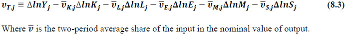 We define the value share of each input as: 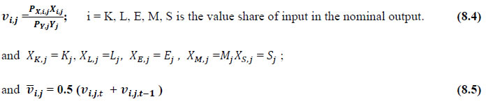 is the two-period average share for input Xi,j  Rearranging equation (8.3), yields the standard growth accounting decomposition of output growth into the contribution of each input and the TFP residual  where the contribution of an input is defined as the product of the input’s growth rate and its two period average value share. We can further decompose the contribution of each input into a quantity and quality component. As discussed earlier, the quality component represents substitution between H components, while the quantity component represents the increases in each detailed input. Our extended decomposition of the sources of output growth is given as follows:  Where Z is the stock of industry capital, Qk is the capital quality, H is number of persons employed and Ql is the quality of labour. The data series at individual industry level constructed for gross value added and gross output, labour input, capital input, intermediate inputs and factor income shares (described in Chapters 2, 3, 4, 5, 6 and 7 respectively) are used to estimate TFPG during the period 1980 to 2019. Labour input is measured by using total person worked along with the labour quality index (see Chapter 4 for a detailed discussion). The series on growth rate in capital services forms the measure of growth in capital input (discussed in Chapter 5). TFPG estimation is done by using the gross output function framework21 (i.e. equation 8.7). 8.2 Methodology for Aggregation across IndustriesWe also provide the TFPG for aggregate economy and two broad sectors, viz. manufacturing and services.22 However, the method of estimation of TFP growth for individual industries described in section 8.1 cannot be readily applied to a higher level of aggregation. The main problem is that gross value of output cannot be added across industries to generate a measure of output at a higher level of aggregation, say for the economy or of any of the broad sectors. Therefore, it becomes necessary to consider appropriate methods of aggregation across industries consistent with the gross output function specification of technology at the individual industry level. We use the Törnqvist index23 for aggregating across the broad sector and total economy. Taking this approach, computations are made for the manufacturing sector, the services sector, and for the aggregate economy. These aggregates are obtained using Tornqvist aggregate of growth rates of real value added, capital input, and labour input. Below, we briefly describe the Törnqvist index. Suppose the aggregate sector J consists of n KLEMS industries (j=1:n). We obtain the output (vale added) and inputs aggregates for sector J as: 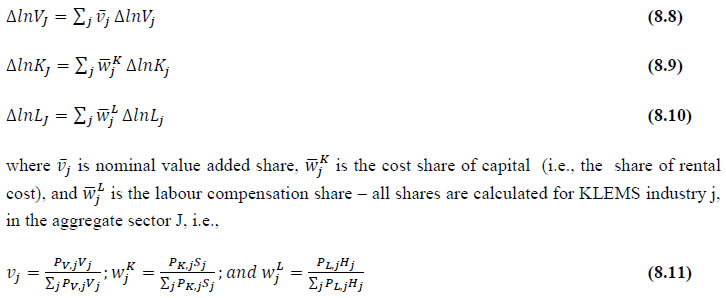 where PV,j is the price of value added in industry j, Vj is the real value added in industry j, PK,j is the rental price of capital in industry j, Sj is the capital stock in industry j, PL,j is the wage rate (price of labour) in industry j, and Hj is the employment in industry j. The aggregate output (real value added) and input growth rates obtained above are then used with the growth accounting equation to obtain the sectoral TFP growth rates. 1 From both aggregated 9 NAS sectors Gross Domestic Product by economic activity statement along with the disaggregated statements of these 9 NAS sectors. 2 In the EUS, the persons employed are classified on the basis of their activity status into usual principal status (UPS), usual principal and subsidiary status (UPSS), current weekly status (CWS) and current daily status (CDS) for quinquennial rounds. refer to Appendix A for detailed definition of UPSS, CWS and CDS. 3 This is also the mid-point of financial year 4 For more detailed discussion on extrapolation and interpolation of the series, readers may refer to KLMES data manual version 2020 released by RBI on its website 5 In PLFS, the earnings by self-employed are also provided, but for consistency with other rounds we have used the same procedure of Mincer equation even for this round. In EU KLEMS (Timmer, et.al., op cit; p 67) it is assumed that the earnings of the self-employed is equal to the earnings of ‘regular' employees. 6 For detailed explanation of Heckman two-step process one may refer to the previous year manual 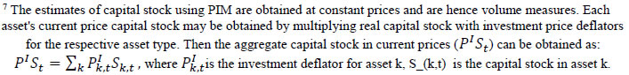 8 This version of the database does not make a distinction between ICT and non-ICT assets, as the industry level data on ICT assets are weak. An attempt to estimate aggregate economy level ICT capital can be found in Erumban and Das (2015). 9 See O’ Mahony and Timmer (2009) for a description of EU KLEMS database 10 This data is not publicly available. However, CSO has been kind to compile this data for the India-KLEMS project. 11 In some years transport equipment was provided as part of the machinery and equipment, categorized as ‘tools, transport equipment and other fixed assets. In such cases, we use transport/tools, transport and other fixed asset ratio in the nearest year to separate transport equipment. 12 A detailed discussion on how the series prior to 2011-2012 were adjusted to match the subsequent series is provided in Box 5.2A in the Appendix. 13 Gross investment is estimated as the difference between book value of asset in period t and in period t-1 and add depreciation in period t to that. 14 This choice is driven by the fact that the first year of availability of ASI data is 1964-65. 15 National Accounts Statistics-Sources and Methods, Chapter 26, CSO (2007), 16 We do not intend to delve into the controversies over the use of internal vs. external rate of return in the context of productivity measurement. This database uses See Erumban (2008a and b) for a discussion on these issues. 17 Reserve Bank of India, Handbook of Indian Statistics, Annual volumes. 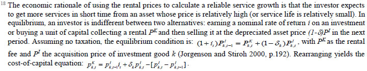 19 The estimation is done at group level rather than individual industries on the consideration that the group level estimates will be more reliable. 20 Consider, the semi-conductor (SC) industry, which is a key input to the computer hardware industry. Much of the output is invisible at the aggregate level because semi-conductor products are intermediate inputs to other industries rather than deliverables to final demand - consumption and investment goods. Moreover, SC plays a role in the improvements in quality and performance of other products like-computers, communication equipment and scientific instruments. Failure to account for them leads us to miss the role of key industries that produce intermediate inputs and importance of intermediate inputs for the industries that use them. (Jorgenson, Ho and Stiroh (2005), Productivity, volume 3). 21 It should be pointed out that an alternate set of estimates of TFPG obtained by using the value-added function framework is also provided in the India KLEMS dataset for which real gross value added is taken as the measure of output and only the two primary inputs are considered, namely labour input and capital input 22 More sophisticated methods of aggregation, such as the application of production possibility frontier approach or the application of direct aggregation is done in research papers written on the basis of the KLEMS dataset prepared. Such estimates of TFP growth are not a part of the database. 23 There exists other approaches to aggregate across broad sectors and industry, a detailed discussion on them can be found in KLEMS data manual version 2020 released by RBI on its website |
||||||||||||||||||||||||||||||||||||


রিজার্ভ ব্যাঙ্ক অফ ইন্ডিয়া মোবাইল অ্যাপ্লিকেশন ইনস্টল করুন এবং সাম্প্রতিক সংবাদগুলিতে দ্রুত অ্যাক্সেস পান!
আমাদের অ্যাপটি ইনস্টল করতে QR কোডটি স্ক্যান করুন


