Over the years, a high level of revenue deficit has led to large fiscal deficits and spiraling debt resulting
in the emergence of a vicious cycle of deficit, debt and debt servicing for the State governments. Increasing
outstanding liabilities also raise questions not only about debt sustainability, but also about intergenerational
equity. Realizing this, the TwFC had suggested a rule based fiscal correction and
consolidation process through the enactment of State level FRLs to contain their key deficits at a
sustainable level over the medium term. In addition, various State governments have set up Consolidated
Sinking Funds and Guarantee Redemption Funds and placed ceilings on guarantees which are
facilitated at containing the magnitude of outstanding liabilities. Recognising the sustainability
issue related to the high level of debt, many of the State governments have placed limits in their FRLs
on the level of debt to be achieved within a stipulated time frame. Consequently, all the parameters of
debt showed an improvement during the period 2005-08. In line with the enlargement of deficits
during 2008-09 (RE) and 2009-10 (BE), the debt level is expected to rise. Market borrowings have
emerged as an important instrument of financing fiscal deficits of the States.
1. Introduction
5.1 The improvement witnessed with regard to
the debt indicators of the States during the recent
past is expected to suffer a setback during the
current year. As a part of counter cyclical measures
to minimize the impact of the global financial crisis
and economic slowdown, the Central government
allowed the States to increase the limit of fiscal
deficit to 3.5 per cent of their respective GSDP
during 2008-09. Thus, States were allowed to raise
additional market borrowings to the extent of 0.5
per cent of GSDP. This additional space was to be
utilised for making capital investments.
Furthermore, Union Budget 2009-10 permitted the
State governments to borrow an additional 0.5 per
cent of their GSDP by relaxing the fiscal deficit
target under FRBM from 3.5 per cent to 4.0 per
cent of their GSDP. In addition to the relaxed GFDGSDP
norm for the State governments, the DCRF
requirement of maintaining revenue deficit at zero
has also been relaxed. The Government of India
has suggested the States to amend their FRLs
accordingly. Despite the additional fiscal space
allowed to the States, 14 States were able to
contain their GFD below 3.5 per cent in 2008-09
(RE) while 13 States proposed to contain the GFDGSDP
ratio below 4.0 per cent in 2009-10 (BE).
Nonetheless, a higher consolidated GFD-GDP ratio
at 2.6 per cent and 3.2 per cent in 2008-09 (RE)
and 2009-10 (BE), respectively—as compared with
1.5 per cent in 2007-08 (Accounts)—is expected
to have implications for the debt sustainability of
the State governments. In this context, allocation
State governments’ expenditure assumes
importance as it would have implications for their
prospective debt servicing capacity.
5.2 In the context of debt sustainability, the
TwFC emphasised the need for fiscal discipline on
the part of the States and suggested that the overall
borrowing programme of a State should be within
a prescribed limit, determined annually, taking into
account borrowings from all sources. The State
governments have been gradually putting in place
institutional mechanisms to contain the level of debt
and also to bring it to a sustainable level by way of
the enactment of FRLs, setting up of Consolidated
Sinking Funds and Guarantee Redemption Funds
and placing ceilings on guarantees. This Chapter
analyses the outstanding liabilities, market
borrowings, contingent liabilities and ways and
means advances-overdraft (WMA-OD) of the State
governments.
2. Outstanding Liabilities10
Magnitude
5.3 The consolidated outstanding liabilities of
the State governments as at end-March 1991 were
placed at Rs.1,28,155 crore ( 22.5 per cent of GDP).
The debt-GDP ratio, which was as low as 20.7 per
cent as at end-March 1997, rose sharply to 32.8
per cent as at end-March 2004 on account of large
and persistent revenue deficits resulting in high
GFD leading to large accumulation of debt and a
concomitant increase in the debt service burden
during the period. Realising the sustainability issue
of the high level of debt, many of the State
governments have placed limits on the level of debt
to be achieved within a stipulated time frame in their
FRLs. The TwFC had recommended for a debt-
GDP ratio of 30.8 per cent to be achieved by the
States at end-March 2010. Furthermore, the TwFC
had recommended an overall cap on borrowings
(3 per cent of GSDP) to be achieved by the State
governments by the end of 2009-10. The TwFC also
recommended the ratio of interest payments to
revenue receipts at 15 per cent to be achieved by
2009-10. The debt relief mechanism prescribed by
the TwFC, incentivised by adherence to the rulebased
fiscal regime by the States helped to contain
the magnitude of outstanding liabilities.
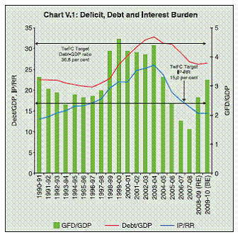
5.4 From the peak level of 32.8 per cent as at
end-March 2004, the debt-GDP ratio of State
governments came down to 26.2 per cent in 2008-09
(RE) (Table V.1, Chart V.1 and Appendix Tables
19-20). The combined IP-RR ratio of the States
declined from 26.0 per cent in 2003-04 to 14.4 per
cent in 2008-09 (RE).
5.5 Notwithstanding the increase in outstanding
level by 10.1 per cent to Rs.1,462,755 crore at end-
March 2009 from Rs.1,328,302 crore at end-March
2008, the debt-GDP ratio declined by 0.6 per cent
over the year. However, outstanding debt is
budgeted to increase to Rs.1,636,403 crore (26.5per cent of GDP) at end-March 2010. Despite this,
the States would be able to contain the debt-GDP
ratio below 30.8 per cent by the end of March 2010
as prescribed by the TwFC.
Table V.1: Outstanding Liabilities of State Governments
(As at end-March) |
(Rs.crore) |
Year |
Amount |
Annual Growth
(Per cent) |
Debt /GDP
(Per cent) |
1 |
2 |
3 |
4 |
1991 |
1,28,155 |
- |
22.5 |
1997 |
2,85,898 |
14.6 |
20.7 |
1998 |
3,30,816 |
15.7 |
21.7 |
1999 |
3,99,576 |
20.8 |
22.8 |
2000 |
5,09,529 |
27.5 |
26.1 |
2004 |
9,03,174 |
14.8 |
32.8 |
2008 |
13,28,302 |
7.0 |
26.8 |
2009 (RE) |
14,62,755 |
10.1 |
26.2 |
2010 (BE) |
16,36,403 |
11.9 |
26.5 |
RE : Revised Estimates. BE : Budget Estimates. ‘–’ : Not applicable.
Source : 1. Budget Documents of the State Governments.
2. Combined Finance and Revenue Accounts of the Union and
State Governments in India, CAG, GoI.
3. Ministry of Finance, Government of India.
4. Reserve Bank records.
5. Union Finance Accounts, GOI. |
 |
Composition of Debt
5.6 The structure of outstanding debt has an
important bearing on interest payment as different
debt instruments carry different rates of interest
depending on the type of borrowing and maturity
structure. It is evident from the Table V.2 and
Chart V.2 that the share of market borrowings has
increased sharply over the years and it would
comprise almost one-third of the total outstanding
liabilities as at end-March 2010. However, there
has been a substantial decline in the share of
loans from the Centre. The dominance of NSSF
has also declined persistently since end-March
2007 and is budgeted to contribute around onefourth
of the total outstanding liabilities as at end-
March 2010. The share of high cost debt
instruments, i.e., public accounts items like small
savings and provident fund in total outstanding
liabilities which had increased marginally to 26.9
per cent at end-March 2008 from 25.5 per cent at
end-March 2005, thereafter showed a declining
trend. Market borrowings comprising one-third of
the outstanding liabilities reflect the low cost debt
segment of the States.
5.7 It is important to highlight here that the budget
documents of the State governments do not provide
sufficient details of their outstanding liabilities
including the amounts under various categories and
associated terms and conditions (such as rate of
interest and maturity structure). This is particularly
evident in the case of negotiated loans from banks
and financial institutions. Consequently, an in-depth
analysis of the debt position of the State
governments remains circumscribed. The detailed composition of outstanding liabilities of State
governments from 1990-91 to 2009-10 (BE) are
presented in Appendix Tables 19 and 20, while the
State-wise composition of outstanding liabilities is
provided in Statements 26-28.
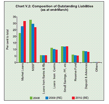 |
Table V.2: Composition of Outstanding Liabilities of State Governments
(As at end-March) |
(Per cent) |
Item |
1991 |
2000 |
2005 |
2006 |
2007 |
2008 |
2009 (RE) |
2010 (BE) |
1 |
2 |
3 |
4 |
5 |
6 |
7 |
8 |
9 |
Total Liabilities (1 to 4) |
100.0 |
100.0 |
100.0 |
100.0 |
100.0 |
100.0 |
100.0 |
100.0 |
1. Internal Debt |
15.0 |
24.8 |
58.7 |
60.9 |
61.5 |
62.1 |
63.9 |
65.1 |
of which: |
|
|
|
|
|
|
|
|
(i) Market Loans |
12.2 |
14.8 |
21.1 |
19.9 |
19.6 |
22.5 |
27.5 |
31.6 |
(ii) Special Securities issued to NSSF |
– |
5.0 |
27.8 |
31.9 |
34.3 |
32.4 |
29.5 |
26.9 |
(iii) Loans from Banks and FIs |
2.0 |
3.4 |
6.7 |
6.3 |
5.6 |
5.4 |
5.4 |
5.3 |
2. Loans and Advances from the Centre |
57.4 |
45.2 |
15.8 |
13.7 |
11.8 |
10.9 |
10.1 |
9.6 |
3. Public Accounts (i to iii) |
26.8 |
29.9 |
25.5 |
25.3 |
26.6 |
26.9 |
25.9 |
25.2 |
(i) Small Savings, State PF, etc. |
13.2 |
15.8 |
12.9 |
12.3 |
12.1 |
12.2 |
12.1 |
12.1 |
(ii) Reserve Funds |
3.7 |
3.9 |
5.2 |
5.5 |
6.3 |
5.9 |
5.5 |
5.1 |
(iii) Deposits & Advances |
10.0 |
10.2 |
7.4 |
7.6 |
8.1 |
8.8 |
8.4 |
8.0 |
4. Contingency Fund |
0.8 |
0.3 |
0.1 |
0.1 |
0.1 |
0.2 |
0.2 |
0.2 |
RE : Revised Estimates. BE : Budget Estimates.
‘–’ : Nil/Negligible/Not applicable.
Source: Same as Table V.1. |
3. State-wise Debt Position
5.8 This section presents State-wise variation
in the level of debt11 among the non-special and
special category States. The State-wise debt-
GSDP position is presented in Table V.3.
Non-Special Category States
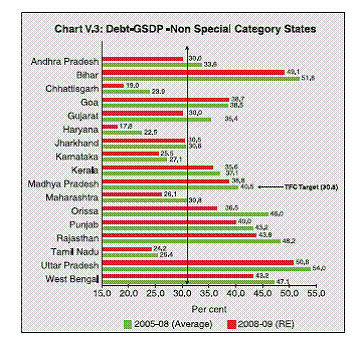
5.9 All the non-special category States, except
Goa, registered an improvement in the debt-GSDP
ratio in 2008-09 (RE) as compared with 2005-08
(Average). Orissa registered the highest
improvement of more than 9.5 per cent of GSDP
during the period, followed by Gujarat (5.4 per cent
each) and Chhattisgarh (4.9 per cent). During 2008-
09 (RE), the debt-GSDP ratio would be as high as
50.8 per cent in case of Uttar Pradesh, followed by
Bihar (49.1 per cent), Rajasthan (43.8 per cent), West
Bengal (43.2 per cent) and Punjab (40.0 per cent).
On the other hand, it would be as low as 17.8 per
cent in the case of Haryana, followed by Chhattisgarh
(19.0 per cent), Tamil Nadu (24.2), Karnataka (25.5
per cent), Maharashtra (26.1 per cent), Andhra
Pradesh and Gujarat (30.0 per cent each) and
Jharkhand (30.5 per cent). Only above eight States
were able to achieve the debt-GSDP target of 30.8
per cent of the TwFC in 2008-09 (RE) (Chart V.3).
5.10 The high burden of interest payments tends
to widen the revenue deficit and in turn the GFD.
Consequently, a vicious circle of deficit, debt and
interest payments becomes formidable. The ratio
of interest payments to revenue receipts, which has
a bearing on debt sustainability, was well below
the TwFC target of 15.0 per cent in the case of
eleven non-special category States, viz. ,Chhattisgarh, Bihar, Haryana, Tamil Nadu,
Karnataka, Andhra Pradesh, Madhya Pradesh,
Uttar Pradesh, Jharkhand, Goa and Maharashtra in 2008-09 (RE). However, in case of six nonspecial
category States inter alia., West Bengal,
Punjab, Gujarat, Kerala, Rajasthan and Orissa the
IP-RR ratio was higher than the prescribed limit of
the TwFC target of 15.0 per cent, although the IPRR
ratio for these six States came down in 2008-09
(RE) as compared to 2005-08 (Average). The
higher share of the IP-RR ratio makes the
expenditure management of State governments
less flexible as a bulk of the resources get preempted
and cannot be used to finance priority
sectors, i.e ., social sector expenditure and
development expenditure.
Table V.3: Debt Indicators of
State Governments |
(Per cent) |
State |
2005-08 (Avg.) |
2008-09 (RE) |
Debt/
GSDP |
Debt/
GSDP |
1 |
2 |
3 |
I. Non-Special Category |
|
|
1. Andhra Pradesh |
33.6 |
30.0 |
2. Bihar |
51.8 |
49.1 |
3. Chhattisgarh |
23.9 |
19.0 |
4. Goa |
38.5 |
36.7 |
5. Gujarat |
35.4 |
30.0 |
6. Haryana |
22.5 |
17.8 |
7. Jharkhand |
30.6 |
30.5 |
8. Karnataka |
27.1 |
25.5 |
9. Kerala |
37.1 |
35.6 |
10. Madhya Pradesh |
40.5 |
38.8 |
11. Maharashtra |
30.8 |
26.1 |
12. Orissa |
46.0 |
36.5 |
13. Punjab |
43.2 |
40.0 |
14. Rajasthan |
48.2 |
43.8 |
15. Tamil Nadu |
25.4 |
24.2 |
16. Uttar Pradesh |
54.0 |
50.8 |
17. West Bengal |
47.1 |
43.2 |
II. Special Category |
|
|
1. Arunachal Pradesh |
76.5 |
74.3 |
2. Assam |
30.4 |
29.2 |
3. Himachal Pradesh |
63.9 |
57.4 |
4. Jammu and Kashmir |
68.9 |
69.7 |
5. Manipur |
79.3 |
77.5 |
6. Meghalaya |
41.4 |
41.5 |
7. Mizoram |
115.8 |
115.9 |
8. Nagaland |
51.1 |
50.1 |
9. Sikkim |
70.3 |
74.1 |
10. Tripura |
47.5 |
37.2 |
11. Uttarakhand |
44.0 |
40.3 |
All States# |
28.9 |
26.2 |
Memo Item: |
|
|
1. NCT Delhi |
19.5 |
15.2 |
2. Puducherry |
31.8 |
42.4 |
Avg. : Average.
GSDP : Gross State Domestic Product.
# : Data for All States are as per cent to GDP.
Source: Based on Budget Documents of the State Governments. |
 |
Special Category States
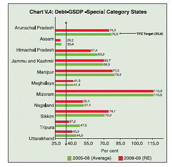
5.11 Out of eleven special category States, seven
States registered an improvement in the debt-
GSDP ratio in the revised estimates of 2008-09
(RE) over 2005-08 (Average). Tripura registered
the maximum improvement of 10.3 per cent in the
debt-GSDP ratio, followed by Himachal Pradesh
(6.5 per cent), Uttarakhand (3.6 per cent),
Arunachal Pradesh (2.2 per cent), Manipur (1.8 per
cent), Assam (1.1 per cent) and Nagaland (1.0 per
cent) in 2008-09 (RE) as compared with 2005-08
(Average). On the contrary, four special category
States viz., Sikkim, Jammu and Kashmir,
Meghalaya and Mizoram registered deterioration in the debt-GSDP ratio during the same period.
During 2008-09 (RE), Mizoram recorded the
highest debt-GSDP ratio of 115.9 per cent, followed
by Manipur (77.5 per cent), Arunachal Pradesh
(74.3 per cent), Sikkim (74.1 per cent) and Jammu
and Kashmir (69.7 per cent). Among all the special
category States, only Assam was able to achieve the
debt-GSDP target of 30.8 per cent during 2008-09
(RE) (Chart V.4). All the special category States,
except Himachal Pradesh, achieved the TwFC
target with respect to IP-RR (15.0 per cent) in 2008-
09 (RE). The IP-RR ratio was the lowest in the case
of Sikkim (4.7 per cent), followed by Arunachal
Pradesh and Meghalaya (6.2 per cent each).
 |
4. Market Borrowings
Consolidated Position
5.12 The State governments issue dated securities
of varying tenures (mostly of 10 years maturity) that
are mostly subscribed by banks and financial
institutions. The share of market borrowings in the
total outstanding liabilities of State governments has
shown a rising trend since end-March 2000 reaching
27.5 per cent as at end-March 2009 as compared to
14.8 per cent at end-March 2000. The greater reliance
on market borrowings has been on account of a
decline in collections under NSSF.
5.13 The share of high cost market loans
(interest rate over 10.0 per cent) of State
governments declined further during 2008-09. As
at end-March 2009, the share of outstanding stock
of market loans with interest rate of 10 per cent
and above declined to 10.1 per cent from 18.4 per
cent as at end-March 2008 (Table V.4). Another
encouraging trend observed in 2008-09 (RE) is
the increase in the share of outstanding market
loans with interest rate of less than 8 per cent.
However, the share of outstanding market loans
with interest rates ranging between 8-10 per cent
increased from 27.3 per cent in end-March 2008
to 34.4 per cent as at end-March 2009.
Allocation of Market Borrowings during 2008-09
5.14 The net allocation of market borrowings
to the State governments as per Reserve Bank
records have increased steadily since 2002-03
(Table V.5 and Appendix Table 21). The total net
allocations increased sharply to Rs.1,14,709 crore
during 2008-09 as compared with Rs.69,015 crore
in the previous year. This was mainly on account
of an additional allocation on account of the NSSF
shortfall and the second stimulus package
amounting to Rs.62,990 crore. Taking into account
repayments of Rs.14,371 crore, the gross allocation of market borrowings amounts to
Rs.1,29,081 crore of which 91.5 per cent was
actually raised by State governments during the
year. During 2008-09, the two States namely,
Chhattisgarh and Orissa did not participate in the
market borrowings programme as compared to
four States, viz., Chhattisgarh, Haryana, Orissa
and Tripura during 2007-08.
Table V.4: Interest Rate Profile of theOutstanding
Stock of State Government Securities
(As at end-March ) |
Range of
Interest Rate |
Outstanding Amount
(Rs. crore) |
Percentage
to
Total |
2008 |
2009 |
2008 |
2009 |
1 |
2 |
3 |
4 |
5 |
5.00-5.99 |
33,825 |
34,825 |
11.3 |
8.7 |
6.00-6.99 |
58,564 |
74,606 |
19.6 |
18.6 |
7.00-7.99 |
69,759 |
1,13,906 |
23.4 |
28.3 |
8.00-8.99 |
76,112 |
1,25,750 |
25.5 |
31.3 |
9.00-9.99 |
5,412 |
12,371 |
1.8 |
3.1 |
10.00-10.99 |
14,418 |
14,418 |
4.8 |
3.6 |
11.00-11.99 |
16,869 |
14,583 |
5.7 |
3.6 |
12.00-12.99 |
23,550 |
11,465 |
7.9 |
2.9 |
13.00-13.99 |
- |
- |
- |
- |
Total |
2,98,508 |
4,01,924 |
100.0 |
100.0 |
Source : Reserve Bank records. ‘–’ : Nil. |
Table V.5: Market Borrowings of
State Governments# |
(Rs. crore) |
Item |
2007-08 |
2008-09 |
2009-10 |
1 |
2 |
3 |
4 |
1. |
Net Allocation |
28,781 |
51,719 |
1,02,458 ^ |
2. |
Additional Allocation |
4,454 |
14,326 |
– |
3. |
Additional Allocation on account of NSSF shortfall |
35,780 |
19,768 |
– |
4. |
Additional Allocation towards second stimulus package |
|
28,896 |
– |
5. |
Total (1+2+3+4) |
69,015 |
1,14,709 |
1,02,458 |
6. |
Repayments |
11,555 |
14,371 |
16,238 |
7. |
Gross Allocation (5+6) |
80,570 |
1,29,080 |
1,18,696 |
8. |
Total Amount Raised (i + ii) |
67,779 |
1,18,138 |
1,14,091 |
|
(i) Tap Issues |
– |
– |
– |
|
(ii) Auctions |
67,779 |
1,18,138 |
1.14,091* |
9. |
Net Amount Raised (8-6) |
56,224 |
1,03,767 |
97,853 |
|
Memo item: |
|
|
|
|
(i) Coupon/Cut-off Yield Range (%) |
7.84-8.90 |
8.39-9.90 |
7.04-8.49 |
|
(ii) Weighted Average InterestRate (%) |
8.25 |
7.90 |
8.06 |
|
(iii) Average Maturity
(in years) |
10.00 |
10.00 |
10.00 |
* Amount raised upto February 8, 2010.
^ : Net Allocation has not been finalised for Andhra Pradesh, Jharkhand
and Maharashtra.
# : Includes the Union territory of Puducherry.
Note : Data on market borrowing as per RBI records may differ from
that reported in the budget documents of the State
Govedrnments.
Source : Reserve Bank records. |
5.15 During 2009-10 (up to February 8, 2010),
the States had raised market loans amounting to
Rs.1,14,091 crore (or 96.1 per cent of the budgeted
allocation) through auctions with a cut-off rate in
the range of 7.04-8.49 per cent. In 2009-10 (up to
February 8 2010), the entire amount of market
borrowings was raised through the auction route
as was the case in the previous two years,
indicating State governments’ intention to raise
market borrowings based on their improved
financial conditions.
5.16 The weighted average interest rate on
market borrowings which had declined since the
mid-1990s up to 2003-04, firmed up to 8.25 per cent
during 2007-08 in line with that of the Central
Government securities, reflecting the general
upward movement in interest rates (Table V.6).
However, thereafter, reflecting the softer interest
rate environment, the weighted average yield of
State government securities issued during 2008-09
and 2009-10 (up to February 8, 2010), was lower
than 2007-08, despite a significant increase in
market borrowings by the States.
5. Liquidity Position and Cash Management
5.17 Keeping in view the cash surplus position
of the State governments, the WMA limits of State
governments have been left unchanged since
2006-07. Accordingly, the extant State-wise normal
WMA limit was fixed at Rs.9,925 crore for 2008-09
(inclusive of Rs.50 crore for the Union Territory of
Puducherry) and the limit has been retained for
2009-10 as well. The rate of interest on normal and
special WMA and OD continued to be linked to the
repo rate (Table V.7).
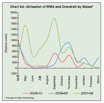
5.18 During 2008-09, the average utilisation of
normal WMA, special WMA and overdrafts by the
States remained low reflecting an improvement in
the overall cash position resulting in a build-up of
high levels of surplus cash balances by most of
the State governments. During 2008-09, six States,
viz., Kerala, Madhya Pradesh, Nagaland, Punjab,
West Bengal and Uttarakhand resorted to WMA as
against eight States, viz., Kerala, Nagaland, Punjab, West Bengal, Himachal Pradesh, Manipur,
Mizoram and Uttarakhand in the previous year.
However, during 2009-10, the situation deteriorated
as the number of States that availed WMA
increased to ten comprising Andhra Pradesh,
Haryana, Kerala, Madhya Pradesh, Punjab, Uttar
Pradesh, West Bengal, Mizoram, Nagaland and
Uttarakhand. During 2009-10 so far (February 11,
2010), Punjab availed of WMA for a maximum 93
days, followed by Nagaland (45 days) and West
Bengal (15 days) (Chart V.5).
Table V.6: Weighted Average Yield of State
Government Securities |
Year |
Yield Range
(Per cent) |
Weighted
Average Yield
(Per cent) |
Gross
Amount
(Rs. crore) |
1 |
2 |
3 |
4 |
1991-92 |
11.50-12.00 |
11.82 |
3,364 |
2000-01 |
10.50-12.00 |
10.99 |
13,300 |
2007-08 |
7.84-8.90 |
8.25 |
67,778 |
2008-09 |
5.80-9.90 |
7.87 |
118,138 |
2009-10* |
7.04-8.49 |
8.06 |
1,14,091 |
* Up to February 8, 2010.
Source: Reserve Bank records. |
Table V.7: Normal WMA Limits – 1996 to 2009 |
Period
|
Amount
(Rs. crore) |
1 |
2 |
i. August 1996 to February 1999 |
2,234 |
ii. March 1999 to January 2001 |
3,941 |
iii. February 2001 to March 2002 |
5,283 |
iv. April 2002 to March 2, 2003 |
6,035 |
v. March 3, 2003 to March 31, 2004 |
7,170 |
vi. April 1, 2004 to March 31, 2005 |
8,140 |
vii. April 1, 2005 to March 31, 2006 |
8,935 |
viii. April 1, 2006 to March 31, 2007 |
9,875 |
ix. April 1, 2007 to March 31, 2008 |
9,925 |
x. April 1, 2008 to March 31, 2009 |
9,925 |
xi. April 1, 2009 to March 31, 2010 |
9,925 |
Source : Reserve Bank records. |
 |
5.19 The monthly average utilisation of overdrafts
(ODs) by the States in 2008-09 was significantly
lower than the previous year. Three States, viz.,
Nagaland, West Bengal and Uttarakhand resorted
to ODs during 2008-09 while Kerala, West Bengal
and Nagaland were the three States that resorted
to ODs in 2007-08. During 2009-10 (February 11,
2010), Punjab availed of OD for 16 days, followed
by Nagaland (13 days) and Uttarakhand and West
Bengal (8 days each) during the year (Statement 38).
5.20 Data on Centre’s (gross) WMA to the State
governments, as reported in the State
governments’ budget documents during 2000-01
to 2009-10 (BE) are set out in Statement 39. The
total amount of such advances has consistently
declined from Rs.3,329 crore in 2002-03 (twelve
States) to Rs.10 crore in 2008-09 (RE) (one State).
However, it is budgeted to increase to Rs.360 crore
in 2009-10 (two States). Assam, among the special
category States, and Kerala among the non-special
category States, have budgeted for such advances
during 2009-10.
6. Contingent Liabilities
5.21 State governments have been issuing
guarantees and letters of comfort on behalf of PSUs
and other institutions (including urban local bodies)
to enable them to raise resources to meet the
requirements of public investment. This is primarily
because the States are not in a position to provide
budgetary support for such investments. Although
contingent liabilities do not form a part of the debt
of the States, in the event of default by borrowing
entities, the States will be required to meet the debt
service obligations. At the same time, nonadherence
to payment obligations committed by the
States with respect to guarantees already provided
by them would have adverse implications on their
sovereign credibility. In view of the fiscal
implications of the rising levels of guarantees, many
States have taken initiatives to place ceilings
(statutory or administrative) on guarantees.
Eighteen State governments have so far fixed
statutory/administrative ceilings on State
government guarantees. Nine States have set up
Guarantee Redemption Funds (GRF).
5.22 The Reserve Bank maintains the
Consolidated Sinking Fund (CSF) and the
Guarantee Redemption Fund (GRF) on behalf of
State governments from contributions made by
them. While the CSF provides a cushion for
amortisation of market borrowing/liabilities, GRF
provides a cushion for the servicing of contingent
liability arising from invocation of guarantees issued
by the State governments with respect to bonds
issued and other borrowings by State level
undertakings or other bodies. The aggregate
outstanding investments in CSF by the 18 State
governments increased to Rs. 24,032 crore at end-
March 2009 from Rs.18,946 crore with respect to
17 States at end-March 2008. As on March 31,
2009, nine States had notified their GRF schemes
and the aggregate outstanding investments in GRF
by these States increased to Rs.3,082 crore as on
March 31, 2009 from Rs.2,805 crore with respect
to 8 States as on March 31, 2008.
5.23 Based on information made available by
select State governments, the outstanding
guarantees of State governments increased sharply
from Rs. 1,32,029 crore (6.8 per cent of GDP) as
at end-March 2000 to Rs.2,19,658 crore (8.0 per
cent of GDP) as at end-March 2004. The
outstanding guarantees of State governments have
declined thereafter to Rs.1,71,058 crore (3.5 per
cent of GDP) as at end-March 2008 (Table V.8 and
Statement 43).
Table V.8: Outstanding Guarantees of
State Governments |
Year
(end-March) |
Amount
(Rs. crore) |
Percentage of GDP |
1 |
2 |
3 |
1992 |
40,158 |
6.1 |
2000 |
1,32,029 |
6.8 |
2004 |
2,19,658 |
8.0 |
2005 |
2,04,426 |
6.3 |
2006 |
1,96,914 |
5.3 |
2007 |
1,54,183 |
3.6 |
2008 P |
1,71,058 |
3.5 |
P : Provisional.
Note : Data pertain to 17 States up to 2005 ,16 States for 2006
19 States for 2007 and 17 States for 2008.
Source: Information received from State Governments and Budget Documents of the State Governments. |
7. Assessment of the Debt Position of State
Governments
5.24 One important issue related to State
finances pertains to sustainability of debt, which
indicates the ability of the State governments to
service their debt obligations. Accordingly, this
section assesses the sustainability of the debt
of State governments in terms of burden of
interest payments and the maturity pattern of
State government securities and issues arising
in the context of liquidity management by the
State governments.
Debt Sustainability
5.25 A trend analysis of the debt-GDP ratio of
State governments shows that it started showing
an upward trend in 1997-98 as States started
implementing the recommendations of the Fifth
Central/State(s) Pay Commission. A sharp rise in
the debt-GDP ratio by 3.3 percentage points to 26.1
per cent was discernible in 1999-2000 as compared
to 22.8 per cent in 1998-99. In addition to the
implementation of the Fifth Central/State(s) Pay
Commission recommendations, this reflected the
States’ rising borrowing needs on account of a fall
in Central transfers in 1998-99 and 1999-2000.
Thereafter, the debt-GDP ratio rose gradually to
32.8 per cent in 2003-04 before moderating
marginally in 2004-05 and 2005-06. Since 2006-07,
at the consolidated level the States have been able
to keep the debt-GDP ratio below the TwFC target of
30.8 per cent. As at end-March 2009, the debt-GDP
ratio stood at 26.2 per cent. As a result of various
schemes and reform measures, there has also been
a significant reduction in the average interest rate on
outstanding debt from 11.17 per cent in 1999-2000
to 7.96 per cent in 2009-10 (BE) (Table V.9).
5.26 Another target envisaged by the TwFC was
with regard to the IP-RR ratio at 15 per cent to be
achieved by 2009-10. An inter-temporal
comparison shows that the IP-RR ratio during 2000-
01 and 2004-05 (EFC award period) was
significantly higher than 18 per cent as prescribed
by the Eleventh Finance Commission (EFC).
Although the IP-RR ratio started declining gradually since 2004-05, the States could bring it within the
TwFC target of 15 per cent in 2008-09 (RE) (14.4
per cent) which would continue to remain so as per
the budget estimates of 2009-10 (14.9 per cent).
The process of fiscal correction and consolidation
seems to have enabled the States to improve their
debt sustainability position in recent years.
Moreover, in addition to the Debt Swap Scheme,
the scheme of conditional debt restructuring and
interest rate relief recommended by the TwFC
encouraged the States to enact FRLs targeting
revenue balance by 2008-09 and GFD at 3 per cent
of GDP by 2009-10. In fact, many of the States
have adopted a specific target for their outstanding
debt-GSDP ratio for a pre-specified date in the future.
Table V.9: Average Interest Rate on
Outstanding Liabilities of
State Governments |
(Per cent) |
Year |
Average Interest Rate* |
1 |
2 |
1991-92 |
8.54 |
1999-00 |
11.17 |
2007-08 |
8.04 |
2008-09 (RE) |
8.00 |
2009-10 (BE) |
7.96 |
RE : Revised Estimates. BE : Budget Estimates.
* : Worked out by dividing interest payments of the current year by
outstanding debt of the previous year
Source : Same as Table V.1. |
5.27 An analysis of achieving the TwFC targets
with respect to debt-sustainability at the State level
shows that at the consolidated level, these targets
have been achieved well ahead of the terminal year
2009-10. However, as per the budget estimates for
2009-10, the States may witness a slight
deterioration in the debt-GDP and IP-RR ratios
albeit remaining within the TwFC limits.
5.28 As far as the growth in outstanding debt is
concerned, it was significantly higher at 10.1 per
cent and 11.9 per cent in 2008-09 (RE) and 2009-
10 (BE) respectively as compared with 7.0 per cent
in 2007-08. Thus, it is important that incremental
debt is used efficiently. In the present context, two
issues are perceived to be important for the States.
First, the States that propose to undertake additional expenditure during the current phase of
the slowdown need to ensure an efficient allocation
of their expenditure so that adequate debt-servicing
capacity is generated. In other words, dedicated
fiscal stimulus packages need to be strictly used
for undertaking capital investments by State
governments. However, budgeted estimates for
2009-10 do not seem to substantiate such a desired
pattern of expenditure. It is evident that the revenue
expenditure(RE)-GDP ratio is estimated to be
higher in 2009-10 (BE) while the capital outlay-GDP
ratio is proposed to be lower. Second, the States
need to review their FRLs keeping in view the currentphase of the slowdown and the need to resume the
path of fiscal correction and consolidation.
Maturity Profile of State Government Securities
5.29 In terms of the maturity profile of the
outstanding stock of State government securities,
more than half, i.e., 53.4 per cent of the outstanding
stock of State governments’ securities as at end-
March 2009 belonged to the maturity bracket of 7
years and above, while 17.1 per cent was under
the 5-7 years bracket and 15.6 per cent was below
the 5 years bracket (Table V.10).
Table V.10: Maturity Profile of Outstanding State Government Securities
(As at end-March 2009) |
State |
Per cent of Total Amount Outstanding |
0-1 years |
1-3 years |
3-5 years |
5-7 years |
Above 7 years |
1 |
2 |
3 |
4 |
5 |
6 |
1. Andhra Pradesh |
5.5 |
10.5 |
16.0 |
14.1 |
53.9 |
2. Arunachal Pradesh |
1.6 |
8.5 |
10.1 |
18.5 |
61.2 |
3. Assam |
4.5 |
10.6 |
15.2 |
20.3 |
49.3 |
4. Bihar |
3.7 |
17.2 |
18.6 |
20.2 |
40.3 |
5. Chattisgarh |
12.1 |
23.6 |
26.6 |
24.7 |
13.0 |
6. Goa |
4.4 |
10.0 |
14.0 |
15.9 |
55.8 |
7. Gujarat |
3.5 |
8.0 |
17.9 |
11.3 |
59.3 |
8. Haryana |
4.4 |
9.0 |
21.8 |
24.3 |
40.5 |
9. Himachal Pradesh |
3.2 |
8.6 |
17.1 |
19.6 |
51.6 |
10. Jammu & Kashmir |
1.7 |
8.0 |
13.5 |
9.7 |
67.0 |
11. Jharkhand |
2.8 |
12.9 |
14.6 |
17.7 |
52.0 |
12. Karnataka |
5.6 |
12.1 |
17.2 |
19.8 |
45.2 |
13. Kerala |
3.5 |
9.9 |
11.5 |
16.6 |
58.4 |
14. Madhya Pradesh |
4.7 |
8.9 |
15.5 |
23.2 |
47.8 |
15. Maharashtra |
2.0 |
5.4 |
12.2 |
13.7 |
66.7 |
16. Manipur |
3.1 |
7.0 |
9.2 |
28.4 |
52.3 |
17. Meghalaya |
5.6 |
11.8 |
9.7 |
22.2 |
50.7 |
18. Mizoram |
3.6 |
8.2 |
15.4 |
20.1 |
52.7 |
19. Nagaland |
5.4 |
12.3 |
12.4 |
20.4 |
42.7 |
20. Orissa |
7.8 |
22.7 |
29.8 |
30.8 |
8.9 |
21. Punjab |
3.5 |
4.8 |
16.1 |
16.0 |
59.5 |
22. Rajasthan |
5.7 |
11.2 |
16.4 |
17.5 |
49.3 |
23. Sikkim |
5.2 |
4.8 |
3.7 |
14.3 |
72.0 |
24. Tamil Nadu |
3.0 |
9.1 |
15.0 |
15.6 |
57.3 |
25. Tripura |
8.1 |
14.0 |
16.7 |
28.3 |
33.0 |
26. Uttarakhand |
2.4 |
5.8 |
29.1 |
25.1 |
33.3 |
27. Uttar Pradesh |
6.0 |
11.3 |
14.2 |
19.9 |
48.7 |
28. West Bengal |
2.2 |
5.7 |
14.3 |
14.7 |
58.8 |
All States |
4.0 |
9.4 |
15.6 |
17.1 |
53.4 |
Source: Reserve Bank records. |
5.30 The maturity profile of market borrowings
shows large repayment obligations from 2012-13
onwards due to a high amount of borrowings during
2002-03 and 2004-05 under DSS. The repayment
obligations will be more than four times in 2017-18
over the previous year on account of the large
magnitude of borrowings during 2008-09 as States
were permitted to borrow 0.5 per cent of their GSDP
on account of the economic slowdown to spur
demand in their economies (Table V.11) (also see
Statements 34-35).
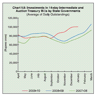
8. Investment of Cash Balances
5.31 Despite the pressure on account of the
implementation of the Sixth Pay Commission/
States’ own Pay Commissions and the prevailing
slowdown, State governments continue to hold
large amounts of surplus cash balances as
reflected in their investments in 14-day Intermediate
Treasury Bills (ITBs) and Auction Treasury Bills
(ATBs). The weekly average investment by the
States in the 14-day ITBs and ATBs during 2009-10
amounted to Rs.83,647 crore (as on January 30,
2010) as compared with Rs.79,128 crore in the
corresponding period of the previous year (Chart V.6).
The upsurge in surplus cash balances at the State
government level since the middle of 2004-05 has implications for the cash management of States as
well as the Central government. The factors
enabling surplus cash balances of State
governments and the possible options for better
cash management are discussed in Box V.1.
Table V.11: Maturity Profile of Outstanding
State Loans and Power Bonds (As at end-March 2009) |
(Rs. crore) |
Year |
State Loans |
Power Bonds |
Total |
1 |
2 |
3 |
4 |
2009-10 |
16,238 |
2,907 |
19,145 |
2010-11 |
15,660 |
2,907 |
18,566 |
2011-12 |
21,993 |
2,907 |
24,900 |
2012-13 |
30,628 |
2,870 |
33,498 |
2013-14 |
32,079 |
2,870 |
34,949 |
2014-15 |
33,384 |
2,870 |
36,254 |
2015-16 |
35,191 |
2,907 |
38,098 |
2016-17 |
31,522 |
1,453 |
32,975 |
2017-18 |
67,442 |
– |
67,442 |
2018-19 |
1,15,524 |
– |
1,15,524 |
2019-20 |
160 |
– |
160 |
2020-21 |
2,103 |
– |
2,103 |
Total |
4,01,924 |
21,690 |
4,23,614 |
Source : Reserve Bank records. |
 |
9. Debt Consolidation and Relief
5.32 To achieve fiscal sustainability, the TwFC
recommended the Debt Consolidation and Relief
Facility (DCRF) with two components: (i) a general
scheme of debt relief applicable to all States; and
(ii) a write-off scheme linked to fiscal performance
with a view to providing an incentive for achievement
of revenue balance by 2008-09. The availing of DCRF
is subject to the enactment of FRL, the quantum of
reduction in RD in each successive year and the
containment of GFD at the level of 2004-05. During
2008-09, twenty-three State governments benefited
from debt relief and twenty-five State governments
benefited from interest relief. The aggregate debt and
interest relief given to the State governments during
2008-09 amounted to Rs.5,748 crore and Rs.3,398
crore respectively. Three State governments, viz.,
Jammu and Kashmir, Sikkim and West Bengal failed
to receive either debt or interest relief during 2008-09.
In the non-special category States, Uttar Pradesh
received the highest debt and interest relief under the
DCRF scheme recommended by the TwFC, followed by Andhra Pradesh and Gujarat during 2008-09
(Statement 48). In the case of special category States,
Assam received the highest amount under the debt
relief facility, followed by Manipur and Tripura.
However, in the case of interest relief Himachal
Pradesh followed by Tripura received the highest
amount during 2008-09.
Box V.1: Surplus Cash Balance of the State Governments: Issues and Challenges
During the late 1990s and in the beginning of the 2000s, State
governments used to avail WMA/OD quite often (with the objective
of covering temporary mismatches in the cash flows of their
receipts and payments) and the level of their surplus cash balance
was quite negligible. However, a rising trend in the cash balances
of States can be observed, particularly since 2004-05. During
2005-06 and 2008-09, the cash surplus balance of all the States
grew at a compound annual growth rate of 57 per cent. Not
surprisingly, a majority of the States stopped seeking short-term
liquidity support from the Reserve Bank through the WMA window
and OD facility. Though the build-up of surplus cash balances
was initially contributed to by an excessive autonomous inflow of
NSSF collections, the phenomenon of high surplus cash balances
has persisted despite a sharp decline in NSSF inflows in recent
years. This might be due to the fact that most States tend to
exhaust their allocated market borrowing limits during the last
quarter of the year and thereby build up surplus cash positions
to be used for the first quarter of the next financial year when
cash inflow generally remains low, but heavy spending by
government departments takes place. The upsurge in the surplus
cash balances at the State government level since the middle of
2004-05 has posed newer challenges for State governments’
financial and cash management. The build-up in the surplus cash
balances has implications for: (i) revenue balances of States; (ii)
Centre’s cash management; and (iii) open market operations of
the Reserve Bank.
Why the States accumulate surplus cash balances instead of
spending? The reason appears to be that States intend to avoid
resorting to ‘WMAs’ or ‘Overdraft’ in the event of major payment
obligations coming forth. In order to avoid any shortage of liquidity
for making any lump-sum payment, they might have built up a
surplus cash position in recent years.
It is observed that around 90 per cent of the surplus cash balances
have been contributed by 13 States, mainly the non-special
category States. Of these, some States have already achieved
their deficit and debt targets well ahead of the stipulated time as
prescribed by the TwFC. Despite the improvement observed in
terms of deficit and debt indicators in a few States, their capital
outlay as a percentage of GSDP is either stagnant or on the lower
side. This indicates that either there is no further capacity in the
States to absorb additional capital spending or they are too
conservative in their approach. The build-up of cash balances
across States has been an outcome of the States’ own efforts to
augment tax revenues and exogenous factors including larger devolution and transfers by the TwFC through shareable Central
taxes and grants.
With regard to the options available for the investment of cash
surplus, a possible option could be using surplus cash balances
at the time of a cyclical downturn, when the States can draw down
their surplus balances to supplement their expenditure
programmes for undertaking countercyclical measures. During
the current phase of the macroeconomic slowdown, it is widely
expected that the States may tend to spend more to boost
domestic demand while there is considerable uncertainty on the
tax collection front, both at the Centre and State levels. Thus,
the high level of cash surplus accumulated at the State level in
recent years seems to provide some headroom to withstand
pressures on finances. The States may be encouraged to build
the capacity of projecting their cash flows on account of receipts
and expenditures and rationalising their surplus cash balances
with the purpose of minimising costs. One possible alternative
may lie in allowing the States to carry forward a part of their
allocated but unavailed amount of borrowings to the next financial
year. This will not only make the States’ borrowing programmes
more need-based but will also provide the States adequate
flexibility to borrow during opportune times in a cost effective
manner. During the boom period, the States may borrow less
and save their unborrowed quota for the downturn phase when
there is the need to spend more to boost the economy. Another
possible alternative could be setting up of a Budget Stabilization
Fund by the States utilizing the durable component of surplus
cash balances which can be used at the time of need. Such an
arrangement would make the States more confident to undertake
countercyclical fiscal policies. Taking cues from Orissa and
Rajasthan, the States may explore the option of repaying high
cost debt by replenishing surplus cash balances.
Further, the States should make serious efforts towards building up
the capacity for better cash management. Apart from greater
coordination among the government entities required for making
realistic assessment of cash needs, States may attempt to avoid
unwarranted build-up of cash surplus by adopting advanced
forecasting and monitoring mechanisms keeping in view the best
practices across advanced economies. As a result of effective cash
management and better synchronisation of cash inflows and outflows,
the States may be able to minimise their borrowing requirements.
This may also help, to some extent, to curb an unwarranted build-up
of cash surpluses by the States which has implications not only for
the Centre’s cash balances but also for monetary policy.
10. Conclusion
5.33 In accordance with the TwFC’s
recommendation, all States (except Sikkim and West
Bengal) enacted FRLs thus limiting their annual
borrowing requirements to a sustainable level. As a
result, from the peak level of 32.8 per cent as at end-
March 2004, the debt-GDP ratio of State governments
came down to 26.2 per cent in 2008-09 (RE) and
below the TwFC target of debt-GDP ratio of 30.8 per
cent by end-March 2010. Further, as against the
TwFC target of interest payment to revenue receipts
(IP-RR) ratio of 15 per cent to be achieved by
2009-10, the combined IP-RR ratio of the States
declined from 26.0 per cent in 2003-04 to 14.4 per
cent in 2008-09 (RE). However, the outstanding debt is budgeted to increase to 26.5 per cent of GDP at
end-March 2010. The IP-RR ratio is budgeted to rise
marginally to 14.5 per cent in 2009-10
5.34 The dominance of NSSF in outstanding
liabilities has also declined persistently since March
2007 and is budgeted to contribute around onefourth
of the total outstanding liabilities as
compared to one-third during 2005-06 to 2007-08.
The share of high cost debt instruments i.e., public
accounts items like small savings and provident
fund in total outstanding liabilities which had
increased to 26.9 per cent in March 2008 from 25.5
per cent in March 2005, thereafter showed a
declining trend. Market borrowings comprising onethird
of the outstanding liabilities reflect the low cost
debt segment of the States.
5.35 In recent years, State governments have
been maintaining large amounts of surplus cash
balances in terms of treasury bills of the Central
Government. Consequently, the dependence of the
State governments on WMA/OD has come down
substantially during the last two years.
10 The outstanding liabilities of State governments have been compiled from various sources including Combined Finance and Revenue
Accounts of the Union and State governments in India, CAG, GoI, Finance Accounts of Union Government, information obtained from
the Ministry of Finance, Reserve Bank records and budget documents of State governments.
11 The detailed State-wise and component-wise break-up of outstanding liabilities is provided in Statements 26-28. The outstanding liabilities
as at end-March 2000 of the three bifurcated States (Bihar, Madhya Pradesh and Uttar Pradesh) have been apportioned to the three
newly formed States (Jharkhand, Chhattisgarh and Uttarakhand), respectively on the basis of their respective proportion of the population.
|
 IST,
IST,


