|
Introducing expenditure quality in intergovernmental transfers: a triple-e framework
Mala Lalvani*, Kumudini S. Hajra, Brijesh Pazhayathodi
ACKNOWLEDGEMENTS
We would like to thank the Reserve Bank of India for the opportunity to undertake the study “Introducing Expenditure Quality in Intergovernmental Transfers: A Triple-E Framework” under the ambit of Development Research Group (DRG).
We would like to record our special thanks to Prof. Ajit Karnik, whose expertise we have drawn upon at every stage of the study. Sincere thanks to Prof. Abhay Pethe, Prof. Avadhoot Nadkarni and Prof. Romar Correa, at the Department of Economics, University of Mumbai, for valuable inputs and suggestions to circumvent innumerable stumbling blocks. We would like to acknowledge the help of Ms. Sriranjani Raja, at the Department of Economics for research assistance.
Within the RBI, we would like to especially thank Dr. R.K. Pattnaik and Mr. B.M. Misra, Advisers, DEAP, RBI for their unstinting support and for their comments and suggestions. We would also like to acknowledge excellent data support provided by Dhirendra Gajbhiye and Ms. Rakhe P.B., Research Officers in the Division of State and Local Finances, DEAP, RBI. We wish to thank the Research Staff of the Development Research Group, RBI for excellent editorial support and suggestions. We would also like to put on record our thanks to an anonymous referee for comments on the previous draft and to the audience who attended the seminar at the RBI for their feedback. Needless to say, sole responsibility for any errors that may remain lies with the authors.
Mala Lalvani
EXECUTIVE SUMMARY
The Thirteenth Finance Commission has for the first time been mandated to consider the need to improve the quality of public expenditure to obtain better outputs and outcomes in its devolution scheme. The present study has sought to introduce, conceptualise and operationalise a scheme for integrating the ‘quality’ dimension of public spending into the devolution scheme of intergovernmental transfers by the Finance Commission.
When speaking of expenditure quality, it is important to draw a distinction between improving the quality of service and improving the quality of public sector budgets (or expenditure quality). Essentially, when measuring expenditure ‘quality’, the orientation is one of providing the ‘necessary’ inputs for improvement in quality of service delivery. For instance, if teachers or doctors positions are filled up and are made available it is providing the necessary condition for improvement in education and health services.
The Twelfth Finance Commission emphasised the significance of improving outputs and outcomes by expenditure re-structuring. This would require some macro issues to be tackled, which must include: (a) re-look at data classification, (b) Centrally sponsored schemes, (c) contingent liabilities, and (d) performance budgeting.
The micro design for improving the ‘quality’ of public spending of State Governments of the Indian federation is presented in our study in a Triple-E framework which has the following basic constituents: Expenditure Adequacy (i.e., re-focusing the primary role of the Government, viz., on the provision of Public Good); Effectiveness (i.e., assessing performance/output indicators for select sectors); and Efficiency of expenditure use (an exercise using Data Envelopment Analysis or DEA which is now a widely accepted methodology internationally for assessing the efficiency parameters).
The study illustrates a scheme of inter-se distribution from an incentive fund, which we would like to label as a “Quality Control Fund” (QCF). Portions of this fund could be kept aside to reward States for their performance on the three aspects of expenditure quality, viz., Expenditure Adequacy, Effectiveness and Efficiency. Devolution from the QCF would be in the nature of a reward or a bonus to the States for their performance on the various aspects of expenditure quality. Since the QCF is an add-on, rewarding States which perform well from this fund would be in the spirit of being incentive compatible without being punitive. Sure, some of the backward States will not receive any substantial amount from this fund, but we are speaking of quality - and quality always comes at a price!
The central message of this study is that a QCF should be created by the Finance Commission. Inter-se distribution from this would be a reward to the States for their performance in the context of expenditure quality. The funds received from this incentive fund should be tied to spending on education and health. Given that the Finance Commission has the mandate of focusing on expenditure quality, it would be a major change of approach if it went a step further and mandated the States to set out some realistic monitorable output targets (which could be reviewed by the next Finance Commission) for the funds that they received from the QCF so as to keep a check on the ‘expenditure quality’ of State governments.
“Public spending is the story of some people spending other people’s money.”
—— (von Hagen, 2005)
I. Introduction
The design of intergovernmental transfers is vital to the functioning of multi-level Government structures. In the Indian context, the significance of Finance Commission transfers can hardly be overestimated as they seal the fate of State Governments’ resource share (for non-plan expenditures) from the federal kitty over the next five years. The motivation of this study is the mandate of the Thirteenth Finance Commission to give due weightage to “The need to improve the quality of public expenditure to obtain better outputs and outcomes” in its devolution scheme. In fact, this facet of ‘expenditure quality’ finds a place in the Terms of Reference (TOR) of the Finance Commission for the very first time. The present study confines itself to examining expenditure quality from the perspective of introducing it in intergovernmental transfers.
Generally speaking, intergovernmental transfers are broadly classified into general purpose (unconditional) and specific purpose (conditional). General purpose transfers are intended to provide general budget support. Such transfers preserve autonomy of sub-national Governments. Specific purpose or conditional transfers are intended to provide incentives to the sub-national Governments for undertaking specific programs. These transfers impose a condition on the kind of expenditure that should be undertaken. In fiscal management jargon these transfers have ‘input-based’ conditionality. Such input-based conditional transfers are considered to be intrusive and unproductive. Shah (2007a) points out that ‘output-based’, conditional transfers, which require attainment of certain results in service delivery while respecting local autonomy, provide a better option. Output-based grants create “incentive regimes that promote results-based accountability culture” (Shah, 2007a, p.13).
The economic rationale for output-based transfers in the Public Management framework is provided by emphasising contract-based management vis-à-vis permanent appointment and strengthening accountability for results. A competitive service delivery environment is created by making finance available on similar conditions to all providers - Government and non-Government. New Institutional Economics also encourages the use of results or output-based transfers. Within this framework, citizens are treated as ‘principals’ and the Government officials as ‘agents’ who act in self interest. Informational asymmetry puts the principals (citizens) at a disadvantage vis-à-vis the agents (Government officials) since processing information about public sector operations is costly. This information asymmetry allows agents to indulge in opportunistic behavior. Hence, output or results-based transfers would enable greater flow of information to the citizens and thereby enhance the accountability culture.
Output-based transfers, which link finance with service delivery, place conditions on results while allowing flexibility in the design of programs. It is important to note that output-based transfers must be linked to outputs rather than outcomes as outcomes are subject to influence by factors beyond the control of public managers. Public managers should be held accountable only for factors under their control. Since conditions attached to the transfers are linked to service delivery in terms of quality of output and access, the manager is free to choose the design of the program and inputs to deliver the results (Shah, 2007a).
This study makes an attempt to integrate, in some measure, the principle of ‘output-based’ intergovernmental transfer scheme into the existing design of Finance Commission transfers. The scheme being suggested here would require an assessment of ‘expenditure quality’ of the State Governments.
Section II of the study introduces the concept of expenditure quality. Section III discusses the various dimensions of expenditure quality from a macro perspective and is sub-divided into two sub-sections: Section III (A) discusses various dimensions of expenditure re-structuring and Section III (B) elaborates on fiscal space that needs to be created for expenditure on public goods. Section IV discusses the micro design of improving expenditure quality and introduces the Triple-E framework that this study advocates. It elaborates on the conceptual issues of the Triple-E framework, viz., Expenditure Adequacy, Effectiveness and Efficiency. Section V puts together the methodological issues and the performance of States within our Triple-E framework; Section VI illustrates one possible way in which the Triple-E Framework could be operationalised by the Finance Commission. Finally, Section VII sums up.
II. Introducing the Concept of Expenditure Quality
Public spending involves delegation, hence leading to a principal-agent relation. Elected politicians can extract rents from being in office, i.e., use some of the funds entrusted to them to pursue their own interests, be it outright corruption, for perks, or simply waste. Voters might wish to eliminate the opportunity to extract rents by subjecting politicians to rules stipulating what they can and must do under given conditions. But the need to react to unforeseen developments and the complexity of the situation makes the voter politician relation resemble an incomplete contract (von Hagen, 2002).
Contracts (formal or informal) between citizens and their political representatives may be, in significant respects, ‘incomplete’ due to some of the relevant information being unobservable by one or more of the contracting parties or even if observable, it may not be specifiable as part of the conditions of a contract. This may be either because the information is too complex to be specified in a legally watertight way, or because it may not be observable by third parties charged with enforcement such as the courts (Seabright, 1996). The nature of goods provided by the Government adds to the complexity of the voter-politician relation.
Only too often it is observed that services provided by the Government fail poor people – in access, in quantity and in quality. This has resulted in traditional weak public trust in public sector performance and delivering of services consistent with citizen preferences. It is increasingly being recognised that economic growth is a necessary but not sufficient condition to accelerate progress in human development. Scaling up would require both a substantial increase in resources and more effective use of all resources.
The World Bank (2004) provides a framework for using resources more effectively by making services work for poor people. The basic constituents of this framework include (i) focusing on those services that have the most direct link with human development – education, health, water, sanitation and electricity; (ii) greater accountability in three key relationships in the service delivery chain: between the poor and service providers, between the poor and policy makers, between policy makers and service providers; (iii) increasing poor clients’ choice and participation in service delivery that will help them monitor and discipline providers; (iv) rewarding effective delivery and penalising the ineffective providers; and (v) systematic evaluation and dissemination of information aimed at empowering the poor. Some of the success stories in service delivery in the Indian context form the focus of a World Bank study (2006). The study elaborates on twenty five cases where major reforms in service delivery occurred. Some well known examples are the simplification of transactions which occurred in case of Andhra Pradesh’s eSeva and Kerala’s FRIENDS; agency reform processes which occurred in case of Stamps and Registration Department of Maharashtra; reform of the Karnataka State Road Transport Corporation; and reform of teacher management in case of Madhya Pradesh. These successes have occurred in individual services and States despite an overall picture of poor service delivery outcomes. A national survey of major public services (elementary schools, public hospitals, public transport, drinking water and public distribution system) by the Public Affairs Centre (PAC) observed that India did well in terms of providing access to basic services but fared poorly in terms of ensuring their quality, reliability and effectiveness (Paul et al, 2004). Some possible reasons for poor service delivery could be the budget being burdened by an expanding salary bill that has crowded out non-salary spending; short tenures caused by premature transfers of officials responsible for public service delivery that hampers continuity; capacity gaps; and weakness in the accountability mechanism (World Bank, 2006).
The framework and suggestions of World Bank (2004) are significant for improving service delivery. However, certain inherent characteristics of public services pose stumbling blocks in the execution of many of these recommendations. A problem with most publicly funded services is that they are relatively complex and characterised by strong information asymmetries. Therefore, it is not feasible – or prohibitively costly – to give detailed instructions for service provision under all imaginable circumstances and to perfectly monitor compliance with such a complete contract or set of instructions. In practice, ‘principals’ are forced to allow ‘agents’ considerable flexibility. Such a principal-agent relationship with the accompanying problems of monitoring tends to result in excessive spending by the agents.
The other property of public goods leading to excessive Government spending has been termed as the common pool problem (von Hagen and Harden, 1996) and was in fact also brought to the fore by Tullock (1959) in his seminal discussion on the majority rule. The common pool property of public budgets leads to excessive spending essentially because those who benefit from targeted public goods and policies are not the only ones who pay for them. In fact, the beneficiaries of most targeted public policies (relatively disadvantaged) would be paying only a small share of the cost. Consequently, politicians tend to target them towards their own constituencies and thus tend to overestimate the social benefit (as they win them votes) and underestimate the social cost (only that fraction which is borne by the specific constituency). This argument is reminiscent of pork barrel politics, which refers to projects, programs and grants that concentrate the benefits in geographically specific constituencies but are financed by broad-based taxation (Weingast, Shepsle and Johnsen, 1981). The Public Choice school points to re-direction of the public resources and policies towards vested interest groups as resulting in excessive Government size (Mueller, 2003).
Given the multiple principal-agent and the common pool property of public services, there is a tendency for budget size to expand and assume ‘Leviathanic’ proportions (Brennan and Buchanan, 1980). Thus, it is imperative that decisions are made not only about ‘what’ is to be done, but equally crucial is the management question of ‘how’ it is to be done (Asian Development Bank, 2001). This is the question at the heart of the body of literature popularised as Public Expenditure Management (PEM). PEM provides a framework of fiscal reform to enhance effectiveness of public policy. A well-functioning PEM system is considered to be a critical pillar of Government efficiency, which would be an important constituent of improving the ‘quality’ for public sector budgets.
At this juncture, it is important to draw a distinction between improving the quality of service and improving the quality of public sector budgets (or expenditure quality). To take the example of electricity service, good quality service would imply regularity of power supply and not having voltage problems. It would also include other aspects such as regularity in meter reading, regularity in issuing bills and grievance redressal (Prayas Energy Group, 2008). Similarly, in the case of education, an improvement in service delivery would mean schools have trained teachers; they must be effective in their jobs; and students should be performing well. In case of health service, it would mean that doctors are readily available in rural areas, they are able to diagnose the problems, and treat the patients with minimal expense and inconvenience. While there can be no doubt about the fact that improvement in ‘quality of service’ should be the target of all expenditure programs, however it is inherently difficult to monitor and measure the quality of service and certainly not possible to quantify and introduce in the devolution scheme of the Finance Commission as is the objective of this study. However, quality of public sector budgets or expenditure quality is certainly possible to include in a devolution scheme for intergovernmental transfers. Essentially, when measuring expenditure ‘quality’, the orientation is one of providing the ‘necessary’ inputs for improvement in quality of service delivery. Hence, if teachers or doctors positions are filled up and are made available, it is providing the necessary condition for improvement in education and health services. Similarly, if transmission and distribution (T&D) losses are targeted to be reduced, it is expected that greater electricity will be available, and hence less will be the load shedding and voltage fluctuations.
Some of the commonly accepted constituents of the quality of the public-sector budgets include (a) reducing committed expenditures in public budgets and focusing on expenditure which is “future-oriented” and growth-oriented; (b) high-quality expenditure in this context may be expenditure on education or research and development; (c) an assessment of the fiscal policy of a country should take into account if necessary structural reforms have been or are in the course of being implemented; and (d) assessing the institutional arrangement, i.e., looking at all relevant fiscal rules, budgetary procedures and – especially in federal States – at the intra-federal structures like equalisation systems (Hoppner and Kastrop, 2005).
The present study suggests assessing the ‘quality’ of public spending of State Governments of the Indian federation in a Triple-E framework. We elaborate on this framework in section IV below when discussing the micro design of improving expenditure quality. However, we would like to reiterate that while monitoring service delivery, empowering civil society and other suggestions made in preceding paras are all vital for improving outcomes and quality of service. The focus of this study is ‘expenditure quality’. The motivation of this study is to obtain a quantifiable measure of ‘expenditure quality’ from the point of view of it being incorporated into the recommendations of the Finance Commission, which is concerned with deciding on criteria for devolution of resources to State Governments.
Before we proceed to the focal point of the study - assessing the quality of expenditures of State Governments, section III below takes a quick look at the macro picture of Central and State Government finances and draws attention to some dimensions of public sector budgets which need to be addressed by either the federal Government or collectively by State Governments, if expenditure quality in general is to improve.
III. Central and State Government Finances: The Macro Picture and Some Basic Issues of Expenditure Quality
Initiation of the reform process in 1991, which marks a watershed in public finances of the Indian economy, resulted in an improvement in the fiscal position of the Central Government and in the consolidated fiscal position of the States as reflected in the major deficit indicators for the period 1990 to 1995. While the Central Government’s fiscal position showed steady improvement, State finances took a turn for the worse since the mid-nineties (Table 1). This could be attributed primarily to the fall in buoyancy of both tax and non-tax revenues. This coupled with a sharp deterioration in performance of State Electricity Boards (SEBs) exacerbated the fiscal stress on the State Governments. Implementation of the award of the Fifth Pay Commission by the State Governments served as the proverbial last straw. This fiscal deterioration continued up to 2003-04.
To rectify the situation, policy makers chose to operate under a rule based fiscal framework and the Fiscal Responsibility and Budget Management (FRBM) Act, 2003 was passed by the Central Government and the State Governments were expected to follow suit. This did not happen naturally, as tying its own hands was not a palatable thought for State politicians. It required the Twelfth Finance Commission to put in place an incentive linked scheme of debt relief for States which passed the Fiscal Responsibility Legislation (FRL). The scheme proved to be a resounding success and presently twenty-six out of twenty-eight States have passed their FRLs (Sikkim and West Bengal are the two exceptions). A listing of the exact years when the various States enacted their FRLs is provided in Table B1, Appendix B. An evolution of key deficit indicators appears in Table 1.
Since the passing of the FRL by the Centre and the State Governments, there has been some reduction in the major deficit indicators. However, for a complete and correct picture, it is essential to go a step further and look ‘below the line’ at the structure and composition of the fiscal correction, especially on the expenditure side of the budget, which is the focal point of this study.
A look at the share of revenue and capital expenditure in total expenditure at the Central Government level indicates that the share of revenue expenditure in total expenditure has increased from 77 per cent in 2004-05 to 83 per cent in 2006-07 (RE), thus implying that the share of capital expenditure has declined from 23 per cent to 17 per cent. For State Governments too, the share of revenue expenditure has risen from 72 per cent to 77 per cent during the same period (i.e., the share of capital expenditure has declined from 28 per cent to 23 per cent). While one is well aware that revenue expenditures are not all ‘bad’ and all capital expenditures are not necessarily ‘good’ (we will have more to say on this later in this section), a falling share of capital expenditure and a rising share of revenue expenditure seems to indicate that fiscal consolidation is of the ‘wrong variety’ (Lalvani, 2008).
Table 1: Deficit Indicators of Centre and States |
(Per cent of GDP) |
|
1985-90 (Avg.) |
1990-95 (Avg.) |
1995-00 (Avg.) |
2000-04
(Avg.) |
2004-07
(Avg.) |
2007-08 (RE) |
2008-09 (BE) |
Centre |
GFD |
7.7 |
6.3 |
5.5 |
5.5 |
3.9 |
3.1 |
2.5 |
|
RD |
2.4 |
3.0 |
3.1 |
4.1 |
2.3 |
1.4 |
1.0 |
|
PD |
4.5 |
2.2 |
1.1 |
0.9 |
0.1 |
-0.6 |
-1.1 |
States* |
GFD |
3.0 |
2.8 |
3.4 |
4.3 |
2.9 |
2.3 |
2.1 |
|
RD |
0.2 |
0.7 |
1.6 |
2.4 |
0.5 |
-0.5 |
-0.6 |
|
PD |
1.6 |
1.1 |
1.4 |
1.5 |
0.4 |
0.1 |
0.1 |
RE: Revised Estimates. BE: Budget Estimates.
RD: Revenue Deficit. GFD: Gross Fiscal Deficit. PD: Primary Deficit.
* Data for the latest three years pertain to 27 State Governments.
Source: 1. Handbook of Statistics on the Indian Economy, 2006.
2. Budget Documents of Government of India and State Governments. |
Another observation on the expenditure composition front is that for States as a whole it is important to note that the expenditure for ‘developmental’ purposes (comprising expenditure on social services, economic services and loans for social and economic services), which has shown signs of improvement in the recent years, is still lower than the levels achieved in the early 1990s. The total developmental expenditure (revenue and capital) as a ratio to GDP, which was 10.7 per cent of GDP during 1990-91 to 1994-95 on an average has declined to 9.4 per cent during 2000-01 to 2004-05. The developmental expenditure to GDP ratio is at 10.1 per cent in 2006-07 (RE), still marginally lower than that attained in the first half of the 90s (Table B2, Appendix B).
The fiscal correction and consolidation process both at the Centre and State levels has essentially been revenue-led on account of robust economic growth and macroeconomic stability coupled with a tax structure based on reasonable rates, fewer exemptions and better compliance. The focus on expenditure has clearly lagged behind. The Twelfth Finance Commission recommended “a multi-dimensional restructuring of Government finances aimed at qualitative and quantitative aspects of managing Government finance” (Twelfth Finance Commission Report, p. 70). The Twelfth Finance Commission recommended restructuring of (i) revenue, (ii) debt, (iii) fiscal transfers, (iv) public sector, and (v) expenditure. Given that the focus of the present study is on the ‘quality’ of expenditures, the following sub-section discusses in some detail the specific aspects of expenditure restructuring that need to be addressed.
III.(A) Expenditure Re-structuring
Expenditure re-structuring would require that the Government focus more on their primary responsibilities rather than thinly spread the resources in many areas where the private sector can provide the necessary services. However, such an improvement in the ‘quality’ of public sector budgets would require some macro issues to be tackled, which will not be possible without the consensus of policy makers and politicians across party lines. These include: (a) re-look at data classification, (b) Centrally sponsored schemes, (c) contingent liabilities, and (d) performance budgeting.
(a) Data Classification Issues
There has been considerable debate about the utility or otherwise of the classification of expenditure into Plan and Non-Plan. It has been argued that this distinction is dysfunctional. This distinction focuses on new schemes/new projects/new extensions to currently running schemes, etc., which alone qualify for being included in the Plan, resulting in neglect of maintenance of the existing capacity and service levels. Thus, while a lot of effort is made by both the Centre and the States to achieve a large increase in Plan size, its impact is often negated by lack of maintenance of the service delivery capacity already created.
The Plan and Non-Plan dichotomy also results in a piecemeal view of resource allocation to various sectors. With the emphasis shifting to social sectors where salary costs are high, routine bans on recruitment for non-plan posts, supposedly to conserve expenditure, causes serious problems for service delivery. Health and education are the two sectors that are badly hit with such bans. Thus, there is a strong case against the use of these categories.
(b) Centrally Sponsored Schemes
The last two decades have seen a massive increase in both the number of Centrally Sponsored Schemes (CSS) as well as funds available under individual schemes. Theoretically, there are two arguments in support of the CSS. Firstly, there is no doubt that there is merit in using Central resources to tackle the specific obstacles that would prevent the achievement of inclusive growth. This is best done by effectively earmarking resources to support State expenditure in particular areas such as rural development, health, education, agriculture and irrigation. Unless this is done it will be difficult to give a special impetus to these critical areas. Second, the mechanism of CSS enables the Centre to address problems as they exist in different States without being constrained by the Gadgil Formula which would otherwise guide the transfer of untied funds. However, herein lies the catch. The virtuous element, while important for flexibility, also gives scope for misuse at the hands of political agents who would be inclined to favour their own political constituencies – a phenomenon popularly known as pork barrel politics.
A large proportion of the funds transferred to the States under CSS are also being routed to the district level bodies directly by the Central Government, bypassing the State Governments. The motivation for this is to avoid delays in administrative approvals and to prevent diversion of CSS funds by the States for supporting their ways and means position. However, overlapping functions by various layers of Government leads to problems of accountability (Garg, 2006).
(c) Contingent Liabilities
The issue of the contingent liabilities of States has come to the fore since the mid 90s when borrowings by State-owned public enterprises were removed from coverage under the ceiling established for States’ market and statutory liquidity ratio (SLR) borrowings. Prior to 1994-95, State enterprises were given separate borrowing allocations each year as part of State-specific global ceilings for SLR and market borrowings. Their SLR qualification status permitted State-controlled enterprises to mobilise funds at relatively low rates of interest. At the same time, the allocation of a specific limit on the amount that could be raised meant there was some control on the extent to which State Governments could issue guarantees. Since the removal of ceiling for State owned enterprises, guarantees have become a convenient means for States to circumvent the ceiling on the quantum of their market borrowings. In addition to use of guarantees for large infrastructure projects, some States have used bonds, financed through special purpose vehicles or corporations with little or no credit records, but with borrowing guarantees from State Governments to raise debt financing for direct budgetary support (McCarten, 2000).
The outstanding guarantees of State Governments have increased from 4.4 per cent of GDP as of end-March 1996 to 8 per cent of GDP as of end-March 2001 and were placed at 7.5 per cent cent of GDP as of end-March 2003. The provisional figures show some improvement on this count with guarantees placed at 5.5 per cent of GDP as of end-March 2006.
A snapshot picture of how the States are placed with respect to guarantees is indicated in Table 2 (State-wise details are given in Table B3, Appendix B). Himachal Pradesh and Maharashtra are two States which have guarantees exceeding 100 per cent of revenue receipts.
Table 2: Position of State Government Guarantees |
(Per cent of Revenue Receipts) |
Outstanding Guarantees as a per cent of Revenue Receipts |
No. of States |
< 25 per cent |
5 |
25 to 50 per cent |
3 |
50 to 100 per cent |
6 |
> 100 per cent |
2 |
Total |
16 |
Source: Computed from State Finances 2007-08, RBI. |
The other significant issue associated with State guarantees relates to borrowings of State public enterprises, especially State Electricity Boards (SEBs), which are incurring losses and show negative returns on capital. Attracting private sector investment for power generation projects in the absence of tariff reform has required granting of rate of return guarantees by many States with counter-guarantees extended by the Government of India. Past guarantees for SEBs and other public enterprises prove to be an obstacle to future reform. If the SEB has raised a large amount of loans guaranteed by the State Government, then the cost of unwinding these commitments as part of privatisation is formidable.
(d) Performance/Outcome Budgeting
A system of performance budgeting by Ministries handling development programmes was introduced to assess the performance against the set goals/objectives. However, it was felt that the document is not able to establish a clear one–to–one relationship between the financial budget and performance. Therefore, in addition to the performance budgeting, the outcome budgeting was introduced. With 2006-07 budget was presented the first outcome budget, which seeks to measure the physical targets achieved on the financial outlays of various Ministries. While presenting the Union Budget 2005-06 in Parliament on February 28, 2005, the Finance Minister had said: “I must caution that outlays do not necessarily mean outcomes. The people of the country are concerned with outcomes. The Prime Minister has repeatedly emphasised the need to improve the quality of implementation and enhance the efficiency and accountability of the delivery mechanism” (Union Budget speech, 2005-06). Clearly, the intention behind the new outcome budget is commendable. The Twelfth Finance Commission, however, expressed the view that performance budgets have receded in importance and that there is a need to bring back performance budgeting as an integral part of the preparation and evaluation of budgets, both for the Centre and the States.
We would like to reiterate that decisions pertaining to the above mentioned four aspects of public sector budgets are crucial for improving the quality of public sector budgets. Data re-classification, increasing accountability and transparent budgetary procedures in the context of CSS, revealing contingent liabilities in the budget and mandating the introduction of performance/outcome budgeting are all best practices which are likely to hurt entrenched vested interests and face much opposition. Hence, it is our firm belief that even though these are hard decisions and require the consensus of policy makers and politicians, these will necessarily need to be imposed.
Understandably the Thirteenth Finance Commission is not likely to have any direct role to play in the issues discussed above as providing incentives to drive any of the above mentioned ‘best practices’, such as introducing performance budgets, may be thought of as impinging on the States’ freedom1 . However, given the significance of the report of the Finance Commission in providing direction to fiscal reforms, we do believe that the Thirteenth Finance Commission can use its prime position to strongly urge the Centre and States to improve on their expenditure management practices and processes and introduce some of the above mentioned best practices.
Expenditure re-structuring by following the best practices mentioned above would enhance the potential that is available to Governments for performing their core function of providing public goods. The potential or the leeway to spend more on core or essential functions is popularly termed as enhancing the ‘fiscal space’. A brief discussion on this is presented in the following sub-section.
III.(B) Virtuous Fiscal Space
“In its broadest sense, ‘fiscal space’ can be defined as the availability of budgetary room that allows a Government to provide resources for a desired purpose without any prejudice to the sustainability of a Government’s financial position”. (Heller, 2005). Revenue raising, expenditure re-prioritisation/rationalisation, borrowings and also policies that raise the potential growth trajectory of an economy are all alternate channels for creating fiscal space (Heller, 2007). Given that the focus of the present study is ‘quality’ of expenditure, it is the expenditure re-prioritisation and rationalisation mode of creating fiscal space that we discuss in some detail.
Rationalisation of expenditure includes reassessing the continued desirability of specific expenditure programs, realising possible efficiency gains in the provision of public goods and services and transfer programs. Creating fiscal space could aim at obtaining an expenditure mix that is more effective in promoting growth (Heller, 2007). Clearly, there can be no ready comprehensive indicators of fiscal space. Some partial indicators could, however, provide some measure of fiscal space. For instance the ratio of Government subsidies to GDP is theoretically an indicator which is a potential candidate for expenditure cuts. Practically, however, subsidies are mostly politically driven and difficult to prune.
For the purpose of this study, we compute a variant of the measure of fiscal space which we label as ‘Virtuous Fiscal Space’ (VFS) available to the Government to spend on core services such as public goods and other developmental services. This is simply measured by netting out committed expenditure. The motivation for obtaining VFS for the Central and State Governments is to get an aggregative measure of the extent to which the Central and State Governments are potentially capable of carrying out their core function – of providing public goods.
VFS has been defined as:
VFS = (RE – CE) / RRC
Where:
RE = Revenue Expenditure
CE = Committed Expenditure (interest payments, administrative expenditure, Pensions and Wages and Salaries)
RRC = Revenue Receipts
 |
Ideally one should compute the VFS by excluding the subsidies component as subsidies are difficult to maneuver (in some senses committed). However, subsidies are not provided for explicitly in the State budgets but there is a large implicit subsidy component, in terms of low cost recovery as has been shown in the Discussion Paper on Government Subsidies by GOI (1997) and in Srivastava et al. (2003). These implicit subsidies, although important, have not been computed for the simple exercise attempted here as it would require detailed data for every State.
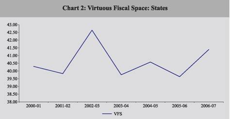 |
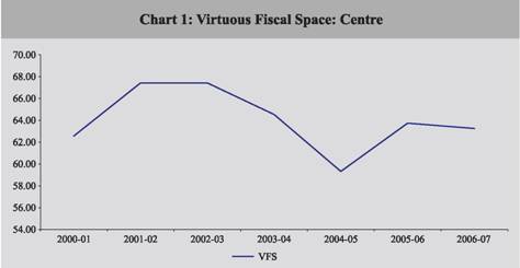
Chart 1 and 2 present a picture of Virtuous Fiscal Space for both Centre and States respectively. In case of the Centre (Chart 1) we observe a clear deterioration in 2003/04 and 2004/05. The passing of the FRBM and improved growth appears to have resulted in a significant improvement in VFS in 2005/06. In 2006/07 once again a marginal deterioration is noticeable with the VFS in 2006/07 being 0.70 percentage points better than it was in 2001/02.
In Chart 2 (i.e., VFS for States) we find 2003/04 as being a year when the VFS shows significant deterioration as was the case even at the Central Government level. Over the next two years (2004/05 and 2005/06) there have been marginal improvement and deterioration. In 2006/07 we once again see some improvement. This improvement could be attributed to the fact that most States had passed their FRLs by then and they were helped by the improved growth scenario. It was only after the Twelfth Finance Commission recommended a debt relief package be used as a ‘carrot’ for inducing the States to pass the Fiscal Responsibility legislation, that most States came forward to avail of the debt relief package and passed their fiscal responsibility legislations from March 2005.
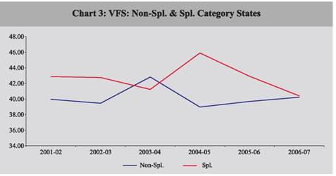
Chart 3 below traces the movement of the VFS separately for the Special and Non-Special category States.
In the context of VFS, the Special category States as a group have by and large been better performers than the Non-Special category States. However, in 2005/06 and 2006/07, the ratio has shown a steady deterioration despite the passing of the FRL by all special category States (barring Sikkim). The reason for this seems to be the increase in the share of administrative expenditure, pensions and wages and salaries by almost one percentage point each vis-à-vis 2004/05. An important point to note at this juncture is that VFS for States is overestimated and not technically very precise to the extent that data on wages and salaries is available for only 15 Non-Special category States and only 4 special category States (in the State Finances, RBI which is our data source for other categories).
 |
A two pronged strategy suggests itself for rectifying the situation: First, create greater fiscal space by curbing contractual or committed expenditures, introducing transparency in budgetary processes, and following some of the other best practices discussed in section III (A) above; and Second, improve expenditure quality and adopt better Public Expenditure Management practices so as to get the maximum impact from the available resources.
IV. Expenditure Quality: A Triple-E Framework
Expenditure ‘quality’ has several dimensions. However, for the purpose of our study we settle on the three facets, which allow us to obtain a quantifiable measure of expenditure ‘quality’. For each of these dimensions we check out how the various States have fared relatively. Such a categorisation of States would enable us design a scheme for integrating expenditure ‘quality’ into the devolution scheme of the Finance Commission. The Triple-E Framework, that we recommend, for assessing the ‘expenditure quality’ of State Governments has the following basic constituents: Expenditure Adequacy ( i.e., re-focusing the primary role of the Government, viz., on the provision of Public Goods); Effectiveness (i.e., assessing performance/output indicators for select sectors); and Efficiency of expenditure use (an exercise using Data Envelopment Analysis or DEA).
IV.(A) Expenditure Adequacy: Adequate Provisioning by focusing on Public Goods and Merit Goods
An economic case for Government intervention in the economy rests on either efficiency grounds or on distributional considerations. The efficiency argument that we draw on here is that of market failures arising in the presence of externalities. Externalities are said to exist when economic activities interact other than through the price system and responses to their existence provides a rationale for Government intervention (Miles et al, 2003).
Public goods provide one example of an externality. They possess the characteristic of Non-Excludability and Non-Rivalry which makes them ‘unmarketable’ or ‘not efficiently marketable’. An implicit assumption for markets to work is that property rights must be well-defined and enforceable. A meaningful assigning of ownership requires that the holder be able to withhold the benefits (costs) associated with the commodity from others, thus requiring excludability. Thus, nonexcludable goods are a subset of collective goods since they cannot be allocated through private markets. In certain instances even when it is possible to exclude, it is important to ascertain whether it is desirable to exclude. When goods are non-rivalrous, the opportunity cost of the marginal user is zero, making exclusion undesirable (even if feasible). Thus, the market cannot play a role in allocating these goods efficiently. Goods with characteristics of both non-excludability and Non-Rivalrous are classified as Pure Public Goods. However, many goods are not ‘pure’ public goods as they possess only one of the two properties (non-rivalry or non-excludability).
Merit Goods refer to those goods where the Government takes a ‘paternalistic’ position and intervenes because it knows what is in the best interest of the individuals better than the individuals themselves. All merit goods can technically be provided privately, but, since many consumers could be priced out, the Government intervenes and provides additional quantities publicly.
In the case of public goods, markets do not function efficiently and could result in under consumption (assuming possibility of exclusion) if a charge is placed on a good which is non-rival. However, if it is not charged for, it would lead to under supply. In the case of merit goods, markets do function but the State intervenes to ensure that sections of the population are not priced out. This provides the rationale for State intervention.
In the present study, we make an attempt to extract and categorise some of the broad expenditure categories of the State Governments (as classified in the RBI’s publication on State Finances) into expenditures for ‘Public Goods’ and for ‘Merit Goods’. It is important to clarify at the outset that these expenditure categories are somewhat broad and hence cannot be classified precisely (as will become evident in subsequent paragraphs). This necessarily implies that we start off by providing our rationale for categorising expenditure categories into public goods or merit goods. (Detailed composition, i.e., the specific sub-major heads and minor heads for each of these broad expenditure categories are available in Appendix A).
The composition of Public Goods and/or Merit goods and the rationale for this categorisation are elaborated upon below:
Public Goods Defined
(1)
Medical and Public Health: This expenditure category has been classified as a public good as it generates positive externalities of enhancing productivity and growth. However, since there is private participation in health care services especially in urban areas, a more precise definition of public goods would consider only rural health services where private participation is absent.2
(2)
Soil and Water Conservation: This expenditure category is classified as a public good as it has the property of non-excludability. It may be possible but not desirable to exclude anyone from the benefits of this expenditure category as consumption would be non-rival.
(3)
Forestry and Wild Life: Like Soil and Water Conservation, this expenditure head too classifies as a public good for the same reason that it may be possible, but not desirable, to exclude anyone from the benefits of this expenditure category as consumption would be non-rival.
(4)
Agricultural Research and Foundation: This includes research and education on irrigation and flood control. Information or knowledge is non-rival, hence this expenditure category would classify as a public good.
(5)
Power: Here markets may not be competitive as there are increasing returns to scale, i.e., the average cost of production declines as the level of production increases. Economic efficiency would thus require that there be a limited number of producers. A regulator may be required to protect the welfare of consumers.
(6) Roads and Bridges: Technically, this expenditure category falls into the category of ‘congestible public good’ and it becomes rivalrous only after a threshold level of users of the roads and bridges.
(7)
Police: This is a pure public good where excludability is neither desirable nor feasible. Public safety and law and order are non-rivalrous too.
Merit Goods Defined: We define Merit Goods to include the following expenditure categories:
(1) Education, Sports, Art and Culture: This expenditure category qualifies as a Merit Good as markets do function (we have a number of private schools) but the Government intervenes with a ‘paternalistic’ and benign motivation to strengthen provision. The conventional reason for public provision of education is distributive considerations. It is felt that education (especially elementary education) for the young should not be dependent on the wealth of their parents.
It is important to note that the broad expenditure head that we consider as Merit Good in our study also includes higher education which technically would not qualify as a ‘Merit Good’ as higher education would be a matter of choice and should be paid for by beneficiaries. Also, under our broad expenditure head we have Art and Culture which includes Public Libraries. Technically, libraries could have congestion costs. So also Museums - In the case of Museums or libraries there is congestion due to crowding. On the cost side, there are maintenance costs to be incurred. If the number of students enrolled doubles, the cost will roughly double. However, all these are certainly expenditures of the Government that have a ‘developmental’ role and are productive. Thus, although technically we should be considering only elementary and secondary education as merit goods, data classification of the RBI’s study on State Finances have required that we make use of a broader classification of Education, Sports, Art and Culture and categorise it as Merit Goods.
(2)
Family Welfare: This expenditure head would clearly qualify as a merit good as the Government adopts a paternalistic role and advises people.
(3)
Water Supply and Sanitation: This expenditure category has been categorised as a merit good as the Government provides it even when a price can be charged, i.e., market can function (meters are installed in many homes). In fact, strictly speaking water is a private good that is publicly provided. If a private good like water were to be freely provided, it would result in over consumption as demand for it would be to the point where the marginal benefit is zero, even though the marginal cost of its provision is positive (it costs to purify water and deliver it from source to individual’s home). Sanitation, on the other hand, is a public good where exclusion is not desirable.
(4)
Welfare of SC, ST and OBC: This expenditure category has been categorised as Merit Good as the objective of this expenditure is purely distributional.
(5)
Labour and Labour Welfare: This expenditure head too has been categorised as Merit Good on account of its distributional objective.
(6)
Social Security and Welfare: This expenditure category has been categorised as a Merit good on account of its distributional objective.
(7)
Nutrition: This expenditure has been categorised as Merit good on account of its distributional objective.
(8)
Relief on Account of Natural Calamities: This expenditure has been categorised as Merit Good on account of its distributional objective.
In our study we obtain the expenditure for each of the twenty-eight States (in per capita terms) on Public Goods and Merit Goods (comprising of the various expenditure categories, the rationale for which was provided above). The reasoning behind this exercise is to see which of the States have made adequate provision for carrying out their primary role of providing public goods. Adequate expenditure provision under each of these categories would be a necessary pre-condition for improvement in expenditure ‘quality’. In order to judge adequacy of expenditure reference has to be made to the needs of the States and cost disabilities that may be quite different for different States. Hence, there is no a priori ‘best’ case. However, given the complexities involved in computing cost disabilities (attempted only by the Australian federation and that too often charged with being arbitrary) and the fact that expenditure needs are assessed by the Finance Commissions in the form of backwardness, area of States, population of 1971 etc. (but are not the concern of this study), assessing the relative performance of States in this context of expenditure on public goods and merit goods is good first approximation to assessing States performance on what we would like to term as ‘core function’. Thus, keeping in mind these caveats, per capita expenditures incurred on Pubic Goods and Merit Goods by States was used as an indicator for Expenditure Adequacy – the first constituent of our Triple-E framework. Details on the performance of States on this count are available in section V.(A).
IV.(B) Effectiveness
Strictly speaking Effectiveness refers to the extent to which outputs of service providers meet the objectives/targets set. A move in the direction of measuring effectiveness requires a shift in focus from inputs to outputs or results of Governments spending. Results-based budgeting approach in the parlance of New Institutional Economics introduces rules and norms that induce (through positive and negative incentives) public representatives and managers to concentrate on a belief that public sector accountability should focus on what the Government does with the money it spends rather than how it controls such expenditure (Andrews, 2005). The results chain based on Shah (2000) is as shown in Fig. 1 below:
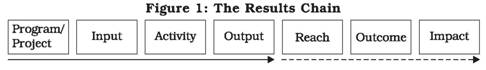 |
The results chain illustrates and helps draw attention to the various dimensions that need to be borne in mind when setting up and/or evaluating any program, viz., output, reach, outcome and impact.
In a performance-based management scheme, accountability is at the core. Andrews (2005) points out that performance-based budgeting has been adopted in Australia, Malaysia, OECD and Singapore. This is not to say that such a scheme is devoid of problems. In fact, he uses the example of South Africa to point out the problems associated with results-based accountability. He points out that the performance targets even though well developed in countries like South Africa, Malaysia, Singapore and in most States of U.S.A are generally kept separate from the actual budget which diminishes its significance. Secondly, in the case of South Africa in particular it has been noticed that targets are poorly detailed and thus lack real world value. The third problem noticed with existing system of performance based budgets is that even where effective targets are provided, the budgets fail to specify who is accountable for these results.
A first step towards introducing an output-based orientation that can easily be implemented is that of linking intergovernmental transfers to outputs (Shah 2007a). The economic rationale for linking intergovernmental transfers was elaborated upon in the Introduction of this study. Output based grants would create an incentive regime that would promote a results based accountability culture. Grants are often given to schools with conditions attached, i.e., for text books, computers, teacher aids, etc. Such conditions linked to inputs are often constraining and may not conform with the priorities of the recipient. However, output-based grants such as imposing conditions on achievement scores on standardised tests and reduction in dropout rates would help achieve accountability for results (Shah, 2007a).
Following the line of reasoning presented in Afonso et al (2005) the present study makes an attempt to compute performance indicators for each of the States. It is important to note that we have made a conscious effort to select output and not outcome indicators. Outcome indicators (such as literacy or infant mortality), while readily available are slow moving indicators, mostly available with a ten year lag. Hence these indicators would not prove to be useful for assessing the current expenditure performance of States. Also, given that placing accountability for such broad outcomes is not possible it would not be correct to use these indicators. Shah (2007a) too points out that output and not outcome indicators must be targeted. It is important to bear in mind that outputs are not independent of private sector provision – so for instance if private sector hospitals are well developed (as is the case in Maharashtra), then the number of public sector hospitals required is less relative to other States where the private sector facilities is relatively low. Bearing in mind this caveat, our study has zeroed in on performance indicators for only four sectors: Education, Health, Law and Order, and Power. In case of health sector we have addressed this issue by focusing on rural health alone (where private sector does not exist). For the other sectors such a fine tuning was not possible on account of data constraints. Undoubtedly, the output indicators to be targeted could be refined in the other sectors too. If targeting outputs is acceptable in principle, then making available relevant data so as to permit precision in selecting the output targets would itself be a challenging (and self-disciplining) task ahead of the policy makers. The present study is merely attempting to suggest a framework. Given the availability of data, the indicators selected for computing the Effectiveness Index are elaborated upon in Section V.(B).
IV.(C) Efficiency
In layman’s terms, efficiency means doing the right thing the right way (van Dooren et al, 2007). Technical efficiency (or operational), the most common efficiency measure, is the one that we compute here. It refers to the output-input ratio compared to a standard ratio, which is considered optimal. Both output and input-oriented efficiency can be defined. Output-oriented efficiency focuses on the maximisation of output for a given set of inputs, or alternatively, input orientation aims at the minimisation of inputs for a given set outputs. Thus the two key objectives of efficiency measurement in the public sector are to trace technical inefficiencies and identifying opportunities for improvements in the way resources are converted into outputs to identify inefficiencies in the mix of production factors (Manning et al, 2006).
Input levels are often predetermined for public services. If we look at the private sector, the budget is an estimate from which companies can deviate, for example, to exploit economies of scale. By contrast, in the public sector, budget is not only an estimate, but also an authorisation. It is an expression of political desire that specific amount of resources be used to attain societal outcomes as well as serve as a guarantee that the overall public budget is in balance. For instance, cultural institutions and environmental agencies usually have fixed inputs. These institutions, however, can attempt to maximise outputs. In other words, they could be output-efficient (Lonti and Woods, 2008).
Measurement of efficiency requires quantitative information on both inputs (or costs) and outputs (or volume) of public service provision. This is a daunting task. A correct measure of the economic value of output requires capturing the quantity and quality of products and services. Most countries measure activities for outputs such as the number of operations in hospitals or number of patrols carried out by the police. According to Atkinson et al (2005), activity indicators reflect what the non-market units are actually doing with their inputs and therefore are closer to the output. However, as the Atkinson report itself points out, this is clearly an imperfect measure. For example, if improved medical treatments reduce the number of operations necessary, then the number of operations performed is no longer a useful indicator since a higher number would imply a decrease of output and productivity. For some collective services, however, activity indicators may be the only indicators that can be found (Atkinson et al, 2005).
There are several other problems that make specification of outputs for the public sector a daunting task. A restriction arises from the nature of the objective function for the public sector which is characterised by multiple criteria. In addition to efficiency, public sector activities often try to achieve equity goals, and there often exists a trade off among these objectives. In addition to the existence of multiple objectives, the public sector differs from the private sector because of the diversity of principals that must be satisfied by agents. The multiplicity of tasks and principals cause serious problems when measuring public output. (Pedraja-Chpparo et al, 2005). Further, the output mix of many public sector organisations includes intangibles. Moreover, measuring outputs can also create incentives to cheat, particularly when output measures directly affect monetary or career incentives. This generally happens in one of the two ways: Data can be deliberately captured in a misleading way, or organisational behaviour can be adapted specifically in order to change the output measures, regardless of other perverse consequences (Van Dooren, 2006). Another important point that needs to be recognised in case of such efficiency analysis is that there are lags between inputs and outputs, and that a marked increase in public spending, such as that which has taken place in recent years, may only show up in improved output indicators at a later date. This applies particularly to Government output such as in education and health. In this situation, measures of productivity, however well based, have to be interpreted carefully.
A large and growing body of empirical research is observed to be examining public sector efficiency. Some of the well known studies which have made international comparison of expenditure performance using the efficiency frontier approach include: Afonso et al (2003) examine public expenditure in OECD; Clements (2002) looks at education spending in Europe; Gupta and Verhoven (2001) study education and health in Africa; St. Aubyn (2002, 2003) analyses health and education spending in Portugal; Afonso and St. Aubyn (2004) examine health and education spending in OECD; and Jacobs, Smith and Andrews (2006) measure efficiency in health care for U.K. Non-parametric techniques of Free Disposable Hull (FDH) and Data Envelopment Analysis (DEA) appear to be most popular with researchers who have addressed this research problem.
DEA is a linear programming model developed by Charnes, Cooper, and Rhodes (1978) that measures relative productive efficiency or productivity of each member of a set of comparable producing units. These units are termed Decision Making Units (DMUs). It is designed to measure relative efficiency in situations where there are multiple inputs and outputs, and there is no obvious objective way of aggregating either into a meaningful index of productivity efficiency. Efficiency is defined as a weighted sum of outputs to a weighted sum of inputs, where the weights structure is calculated by means of mathematical programming and constant returns to scale (CRS) are assumed. Subsequently Banker, Charnes and Cooper (1984) developed a model with variable returns to scale (VRS). The choice between CRS and VRS often poses problems. In the present study, we settled for CRS as the objective was to assess productivity irrespective of the scale of operation (Jacobs, Smith and Street, 2006).
The most common efficiency concept that is sought to be measured is technical efficiency: the conversion of inputs into outputs relative to best practice. In other words, given current technology, there is no wastage of inputs whatsoever in producing the given quantity of output. An organisation operating at best practice is said to be 100 per cent technically efficient and is assigned an efficiency parameter of one. Thus, inefficiency of the other DMUs is relative to the efficient DMU.
DEA has been recognised as a valuable analytical research instrument and a practical decision support tool. It has been credited for not requiring a complete specification for the functional form of the production frontier nor the distribution of inefficient deviations from the frontier. One of the primary advantages of DEA over other techniques is that each input or output can be measured in its natural physical units. As a result, there is no need for a weighting system that reduces those units into any single unit measure. This makes it particularly suitable for analysing the efficiency of Government service providers, especially those providing human services where it is difficult or impossible to assign prices to many of the outputs. However, like any empirical technique, DEA is based on a number of simplifying assumptions that need to be acknowledged when interpreting the results of DEA studies. Being a deterministic rather than statistical technique, DEA produces results that are particularly sensitive to measurement error; DEA only measures efficiency relative to best practice within the particular sample. However, despite these limitations, DEA is a useful tool for examining the efficiency of service providers (http://www.pc.gov.au/data/assets/pdf_file/0006/62088/dea.pdf).
The present study uses the DEA3 to obtain efficiency parameters which give us our Efficiency Index. The Efficiency parameters are presented in sub-section V. (C). Our empirical exercise considers the same four expenditure categories which were emphasised when computing the Effectiveness Index, viz., Education, Rural Health, Police and Power.
V. Operationalising the Triple-E Framework
The empirical exercises carried out in this study are illustrative – the primary objective of the exercises is to operationalise and integrate the Triple-E framework - Expenditure Adequacy, Effectiveness and Efficiency - into the devolution scheme of the Finance Commission.
Data Sources
The State Finances publication of RBI provides a comprehensive and consistent data set and hence has been the main data source used for this study in the case of fiscal data for States. However, the broad classifications used pose problems when attempting to precisely define expenditures on public goods (as was discussed when defining Public and Merit Goods in section IV above). Nevertheless, since the purpose of identifying public/merit goods expenditure in this study is to identify priority areas of expenditure for the Government or, in other words, improve ‘quality’ of expenditure, this objective of ours is adequately served even with the broad expenditure categories (and somewhat loosely defined expenditures on public goods) as are available in State Finances, RBI.
The need for a more detailed expenditure classification was felt when attempting to obtain a measure of efficiency using DEA. Hence, for the section of the study using DEA we have had to switch data sources and turn to the Finance Accounts (FAs) brought out by the Accountant General of various States. Since not all of the FAs are available in the public domain nor are they readily available for a few years, the exercise had to be limited to using one year’s data alone. The exercise using the data from FAs thus suffers from the limitation that all cross-sectional exercises are prone to distortions due to the fact that the selected year could be an outlier for some cross-section units. Ideally, an average of a few years (as has been done in case of identifying expenditure on public goods using State Finances) would always make the exercise more robust.
The output indicators have been obtained from www.indiastat.com and State analysis series of CMIE. The lack of systematically and consistently organised and compiled data for output indicators is in itself indicative of the fact that the Indian policy makers have thus far focused on financial aspects and not paid much heed to the impact which the resources have had in terms of outputs. Lack of systematic data compelled us to fall back on using the data for the latest year available. If expenditure quality is to improve then there has to be shift in the focus from merely resources to be spent to the targets to be achieved and the outputs attained. The Finance Commission can play a major role in initiating this shift in focus.
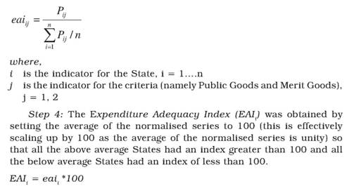
V.(A) Expenditure Adequacy Index
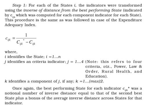
Expenditure Adequacy forms the first component of our Triple-E framework. It captures a necessary condition of the Government carrying out its basic role of providing public goods. Adequate expenditure on essential services would be a prerequisite for improving on outputs and outcomes. Thus adequacy of expenditure on Public Goods and Merit Goods determines our Expenditure Adequacy Index. The step-wise procedure for obtaining the Expenditure Adequacy Index (EAI) and a listing of the expenditure categories is provided below:
Step 1: We identify the various expenditure categories which could be classified as Public Goods and Merit Goods (as listed above), indicating the ‘meritorious’ component of the budget (Table 3). We consider the per capita expenditure for each State on these categories and average it over four years 2003/04 to 2006/07 (RE) in order to avoid any sharp outliers.
Table 3: Composition of Public and Merit Goods |
Expenditure Per capita on Public Goods include: |
(i) |
Medical and Public Health, |
(ii) |
Soil and Water Conservation |
(iii) |
Forestry and Wild Life, |
(iv) |
Agricultural Research and Education |
(v) |
Power |
(vi) |
Roads and Bridges |
(vii) |
Police |
Expenditure Per capita on Merit Goods include: |
(i) |
Education, Sports, Art and Culture, |
(ii) |
Family Welfare |
(iii) |
Water Supply and Sanitation |
(iv) |
Welfare of SC, ST and OBC Labour and Labour Welfare, |
(v) |
Social Security and Welfare |
(vi) |
Nutrition, Relief on Account of Natural Calamities |
Note: For detailed break-up of the above major heads into minor heads see Appendix A. |
 |
The Expenditure Adequacy Index (EAI) for the non-special and special category States have been tabulated in Table 4A and 4B. The basic data used for the computation of the index is listed in Table B5 (Appendix B)
.
We find that the first five rankers among the non-special category States have an index greater than or equal to 100, i.e., their performance on this count is average and better than the average. These include Goa, Haryana, Maharashtra, Karnataka and Tamil Nadu. The three special category States that have an index in excess of 100 are Sikkim, Mizoram and Arunachal Pradesh. It is also interesting to note that the special category States exhibit considerable variability in EAI, a feature not seen for the non-special category States. The coefficient of variation was much less for non-special category States than special category States.
A comparison of the performance of the States on this count along with their performance on the effectiveness and efficiency indicators in subsequent sub-sections would provide us with a fair idea about whether the States spending adequately (relatively) also fare well on output and efficiency.
Table 4A: Expenditure Adequacy Index and State Ranks (Non-Special Category States) |
State |
Expenditure Adequacy Index (EAI) |
Rank |
Andhra Pradesh |
99 |
8 |
Bihar |
79 |
17 |
Chattisgarh |
93 |
10 |
Goa |
202 |
1 |
Gujarat |
98 |
9 |
Haryana |
108 |
2 |
Jharkhand |
91 |
12 |
Karnataka |
100 |
4 |
Kerala |
99 |
6 |
Madhya Pradesh |
86 |
14 |
Maharashtra |
104 |
3 |
Orissa |
87 |
13 |
Punjab |
99 |
7 |
Rajasthan |
92 |
11 |
Tamil Nadu |
100 |
5 |
Uttar Pradesh |
83 |
15 |
West Bengal |
80 |
16 |
Coefficient of Variation |
1.16 |
|
Table 4B: Expenditure Adequacy Index and State Ranks (Special Category States) |
State |
Expenditure Adequacy Index (EAI) |
Rank |
Arunachal Pradesh |
144 |
3 |
Assam |
27 |
11 |
Himachal Pradesh |
43 |
5 |
Jammu and Kashmir |
47 |
4 |
Manipur |
42 |
6 |
Meghalaya |
35 |
9 |
Mizoram |
337 |
1 |
Nagaland |
41 |
7 |
Sikkim |
313 |
2 |
Tripura |
37 |
8 |
Uttarakhand |
33 |
10 |
Coefficient of Variation |
0.27 |
|
V.(B) Effectiveness Index
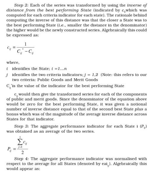
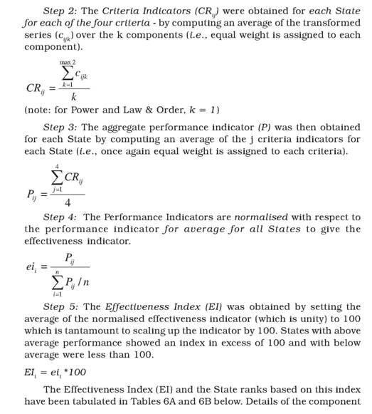
The Effectiveness Index (EI) is the second component of our Triple-E framework. It captures the performance of the States on specific output indicators and follows a similar procedure as was outlined above for the Expenditure Adequacy Index. However, here some additional steps were required as two of the four criteria (education and health) had more than one component. Hence, component indicators needed to be aggregated to obtain criteria indicators which needed to be further aggregated to obtain performance indicators and then to work out the effectiveness index.
It is important to select the output indicators with care. Our concern when identifying these output indicators was that they should be relatively quicker moving output indicators which are available with a lag of at most a couple of years as against the slow moving outcome indicators which are available with a lag of almost ten years. This is an important consideration if these indicators are to be incorporated into the devolution scheme of intergovernmental transfers by the Finance Commission. We would also like to draw attention to the fact that our output indicators (like our expenditure adequacy indicators) once again aim at providing the necessary condition for improving expenditure quality. So filling up sanctioned posts of doctors and availability of health centres are expected to improve the health status. Similarly, a reasonable teacher pupil ratio is expected to help improve the quality of education. A listing of the four criteria and their respective components has been listed out in Table 5. The steps are similar to those followed in case of Expenditure Adequacy Index. However, here there are four criteria (Power, Law & Order, Rural Health, and Education) and each of these criteria has one or two components. Hence, an additional step of computing the criteria indicators from the component indicators was required. A listing of the specific output indicators and the step-wise details of the procedure are as follows:
Table 5: Criteria and Components for Effectiveness Index |
Criteria |
Components |
(A) Health Indicator |
a) Shortfall in PHC/CHC/SUBC as per norms |
b) Doctors per PHC |
(B) Education Indicator |
a) Enrolment ratio in secondary education |
b) Pupil Teacher Ratio |
(C) Law and Order Indicator |
a) Incidence of Crime |
(D) Infrastructure Indicator (Power) |
a) T&D losses as per cent of availability |
PHC: Primary Health Centre. CHC: Community Health Centre.
SUBC: Sub-Centre. T&D: Transmission and Distribution. |
indicators, performance indicators and EI for the special and non-special category States have been tabulated in Table B.6 in Appendix B.
Table 6A: Effectiveness Index and State Ranks (Non-Special Category States) |
State |
Effectiveness Index (EI) |
Rank |
Andhra Pradesh |
79 |
8 |
Bihar |
30 |
17 |
Chattisgarh |
70 |
9 |
Goa |
123 |
7 |
Gujarat |
133 |
5 |
Haryana |
43 |
14 |
Jharkhand |
125 |
6 |
Karnataka |
212 |
2 |
Kerala |
197 |
3 |
Madhya Pradesh |
33 |
15 |
Maharashtra |
48 |
13 |
Orissa |
54 |
11 |
Punjab |
59 |
10 |
Rajasthan |
142 |
4 |
Tamil Nadu |
269 |
1 |
Uttar Pradesh |
31 |
16 |
West Bengal |
51 |
12 |
Coefficient of Variation |
0.71 |
|
Table 6B: Effectiveness Index and State Ranks (Special Category States) |
State |
Effectiveness Index (EI) |
Rank |
Arunachal Pradesh |
86 |
7 |
Assam |
19 |
9 |
Himachal Pradesh |
91 |
6 |
Jammu and Kashmir |
118 |
3 |
Manipur |
92 |
5 |
Meghalaya |
19 |
10 |
Mizoram |
97 |
4 |
Nagaland |
13 |
11 |
Sikkim |
273 |
1 |
Tripura |
219 |
2 |
Uttarakhand |
72 |
8 |
Coefficient of Variation |
0.81 |
|
We find that Tamil Nadu, Karnataka, Kerala, Rajasthan, Gujarat, Jharkhand and Goa among the non-special category States have an index exceeding 100. Thus, Haryana and Maharashtra which were above average performers on the expenditure adequacy index, fare badly on the effectiveness index. Among the special category States, Sikkim, Tripura and Jammu and Kashmir have Effectiveness Index exceeding 100. Mizoram and Arunachal Pradesh which were above average on expenditure adequacy fall below average on the effectiveness count. Once again the Coefficient of variation is seen to be higher for the special category States although the difference is not as much as was observed in case of the Expenditure Adequacy Index.
This observation serves to underline the point that merely high expenditures do not translate into better outputs and outcomes. Thus a special focus on output is crucial when earmarking resources.
V.(C) Efficiency Index
The Non-Parametric Data Envelopment Analysis (DEA) technique was used to obtain efficiency parameters using the same four criteria considered for the Effectiveness Index, viz., Rural Health, Education, Power, and Law and Order. The “inputs” are the expenditure on these four categories. It is important to note that for two of the criteria, viz., Power and Police, the expenditure data are the same as used in case of the expenditure adequacy index (i.e., an average of four years was considered), but for rural health service and primary and secondary education we obtained more precise expenditures for this sub-category from the Finance Accounts of the various States. For these, however, only one year’s data (either 2006-07 or 2005-06) as was available was considered. Undoubtedly, this would affect the precision of the results obtained. However, since the motivation for the empirical exercise carried out in this study is to illustrate and operationalise the Triple E Framework, a lack of precision in availability of data did not constrain us. The expenditure data (i.e., the inputs) have been considered in real prices (GSDP deflator was used). The inputs and outputs for each of the four criteria have been tabulated in Table 7.
In case of DEA, the output indicators were transformed so that “more is better”. Thus, in case of pupil-teacher Ratio, T & D losses and incidence of crime, the inverse was used so that ‘more is better’. The Efficiency parameters for each of the criteria have been tabulated in Table B7 (Appendix B). The Efficiency Index and the State rankings are listed in Table 8A and 8B.
Goa, Orissa, Chhattisgarh, Jharkhand and West Bengal are the non-special category States which have an efficiency index surpassing the average of non-special category States. The variability of the Efficiency Index is once again seen to be higher for the special category States.
Table 7: Inputs and Outputs in DEA Exercise |
Criteria |
Input |
Output |
(A) Infrastructure (Power) |
Total Expenditure on Power (constant p) (average 2003-04 to 2006-07) |
(a) Electricity generated |
(b) T&D losses % of
availability (100-losses) |
(B) Health |
Total Expenditure on Rural Health Services (constant p) (average 2003-04 to 2006-07) |
(a) No. of PHCs |
(b) No. of SUBCs |
(c) No. of CHCs |
(d) Doctors in PHCs |
(C) Education |
Total Expenditure on Secondary Education (constant p) (average 2003-04 to 2006-07) |
(a) Pupil teacher ratio (inverse) |
(b) Gross enrolment ratio in secondary education |
(D) Law and Order (criteria 4) |
Total Expenditure on Police (constant p) (average 2003-04 to 2006-07) |
(a) Police strength |
(b) Incidence of crime (inverse) |
PHC: Primary Health Centre. CHC: Community Health Centre.
SUBC: Sub-Centre. T&D: Transmission and Distribution.
Source: Outputs from www.indiastat.com; Expenditure on power and police from State Finances, RBI;
Expenditure on rural health and elementary and secondary education from Finance Accounts, CAG, various years. |
Table 8A: Efficiency Index and State Ranks (Non-Special Category States) |
State |
Efficiency Index (EFI) |
Rank |
Andhra Pradesh |
77 |
10 |
Bihar |
71 |
17 |
Chattisgarh |
173 |
3 |
Goa |
195 |
1 |
Gujarat |
79 |
8 |
Haryana |
81 |
6 |
Jharkhand |
142 |
4 |
Karnataka |
79 |
9 |
Kerala |
72 |
14 |
Madhya Pradesh |
76 |
13 |
Maharashtra |
76 |
12 |
Orissa |
174 |
2 |
Punjab |
71 |
16 |
Rajasthan |
77 |
11 |
Tamil Nadu |
81 |
7 |
Uttar Pradesh |
71 |
15 |
West Bengal |
105 |
5 |
Coefficient of Variation |
0.42 |
|
Table 8B: Efficiency Adequacy Index and State Ranks (Special Category States) |
State |
Efficiency Index (EFI) |
Rank |
Arunachal Pradesh |
245 |
2 |
Assam |
75 |
6 |
Himachal Pradesh |
87 |
5 |
Jammu and Kashmir |
38 |
7 |
Manipur |
34 |
8 |
Meghalaya |
90 |
4 |
Mizoram |
205 |
3 |
Nagaland |
14 |
11 |
Sikkim |
260 |
1 |
Tripura |
21 |
10 |
Uttarakhand |
31 |
9 |
Coefficient of Variation |
0.92 |
|
Juxtaposing the performance of various States on the basis of the three indices that we have identified throws up some interesting and significant observations. We tabulate below the top five rankers, the bottom five rankers and the average performers for each of the criteria in Table 9A and 9B.
Table 9A shows that Maharashtra and Haryana, while among the top five in the expenditure adequacy index, are among the bottom five in the effectiveness index and average performers in the efficiency index. Goa which was the top ranker in expenditure adequacy was an average performer on the effectiveness front but a good performer on the efficiency front. Karnataka and Tamil Nadu, which were among the top five in the expenditure adequacy, were also among the top five in the effectiveness index, but average performers in the efficiency index. Bihar, Uttar Pradesh and Madhya Pradesh are consistently poor performers on all three indices.
Table 9A: Summary Rankings: Non-Special Category States |
Index |
TOP 5 |
AVERAGE |
BOTTOM 5 |
Expenditure Adequacy Index (EAI) |
Goa |
Jharkhand |
Bihar |
Haryana |
Rajasthan |
West Bengal |
Maharashtra |
Chattisgarh |
Uttar Pradesh |
Karnataka |
Gujarat |
Madhya Pradesh |
Tamil Nadu |
Andhra Pradesh |
Orissa |
|
Punjab |
|
|
Kerala |
|
Effectiveness Index (EI) |
Tamil Nadu |
West Bengal |
Bihar |
Karnataka |
Orissa |
Uttar Pradesh |
Kerala |
Punjab |
Madhya Pradesh |
Rajasthan |
Chattisgarh |
Haryana |
Gujarat |
Andhra Pradesh |
Maharashtra |
|
Goa |
|
|
Jharkhand |
|
Efficiency Index (EFI) |
Goa |
Maharashtra |
Bihar |
Orissa |
Punjab |
Punjab |
Chattisgarh |
Rajasthan |
Uttar Pradesh |
Jharkhand |
Andhra Pradesh |
Kerala |
West Bengal |
Karnataka |
Madhya Pradesh |
|
Tamil Nadu |
|
|
Haryana |
|
A similar grouping for special category States, have been reported in Table 9B.
Table 9B shows that Sikkim is a consistently good performer. It ranks among the first two on all three indices. Arunachal Pradesh and Mizoram rank among the top three in two out of three indices and are seen to be average performers on the third index.
Table 9B: Summary Rankings: Special Category States |
Index |
TOP 3 |
AVERAGE |
BOTTOM 3 |
Expenditure Adequacy Index (EAI) |
Mizoram |
Tripura |
Assam |
Sikkim |
Nagaland |
Uttarakhand |
Arunachal Pradesh |
Manipur |
Meghalaya |
|
Himachal Pradesh |
|
|
J & K |
|
Effectiveness Index (EI) |
Sikkim |
Uttarakhand |
Nagaland |
Tripura |
Arunachal Pradesh |
Meghalaya |
J & K |
Himachal Pradesh |
Assam |
|
Manipur |
|
|
Mizoram |
|
Efficiency Index (EFI) |
Sikkim |
Manipur |
Nagaland |
Arunachal Pradesh |
J & K |
Tripura |
Mizoram |
Assam |
Uttarakhand |
|
Himachal Pradesh |
|
|
Meghalaya |
|
The preceding analysis for both non-special and special category States shows that there is a clear disconnect between spending (i.e., expenditure adequacy) and performance on output indicators and on efficiency, the two other components of expenditure quality. One can hardly over-emphasise the importance of expenditures having the necessary desired impact in terms of output and efficient utilisation of resources. Thus, the inclusion of expenditure quality in the TOR of the Thirteenth Finance Commission is a welcome addition. The Thirteenth Finance Commission is ideally placed to bring the concern of expenditure quality to the Centre stage. A possible scheme of integrating the three indices of expenditure quality discussed above into the devolution pattern of the Finance Commission has been outlined in section VI.
VI. Integrating Expenditure Quality in the Devolution Scheme of FC
The Twelfth Finance Commission initiated the idea of tied grants for health and education. A two step normative procedure was used to identify the States which were seen to perform poorly vis-à-vis the group average and a grant was assigned to these States to cover some proportion of the distance. Using this procedure, the Twelfth Finance Commission provided grants to eight States. Thus, a tied grant was made available for education and health to States that were in ‘need’ of greater resources. We would like to see the Thirteenth Finance Commission extend this idea of tied grant for education and health to all States and mandate the setting out of output targets to be attained. We would like to advocate that the needs-based tied grant for education and health introduced by the Twelfth Finance Commission must be persisted with. Over and above this, we would like to see the Thirteenth Finance Commission introduce an incentive fund, the allocation from which would also be tied to spending on education and health by the States and outputs to be attained from these resources identified at the outset. It is true theoretically that tied grants impinge on the freedom of sub-national Governments and go against the spirit of a federal setup. However, for Merit Goods and Public Goods (like health and education), we do believe that a ‘paternalistic’ attitude by the Finance Commission is justified.
The inter-se distribution from the incentive fund, which we would like to label as a “Quality Control Fund” (QCF) would be based on the three aspects of expenditure quality that we have identified, viz., Expenditure Adequacy, Effectiveness and Efficiency. It would be in the nature of a reward or a bonus to the States for their performance on the various aspects of expenditure quality. Rewarding performance would be the single point objective of the QCF. Since the QCF is an add on, rewarding States which perform well from this fund would be in the spirit of being incentive compatible without being punitive. Sure, some of the backward States will not receive any substantial amount from this fund, but we are speaking of quality - and quality always comes at a price!
This section outlines a possible channel for integrating expenditure quality in the devolution scheme of the Finance Commission. The procedure outlined here follows the methodology set out by Karnik, Pethe and Karmarkar (2001) which set out a quantitative framework for the Second State Finance Commission of Maharashtra. We illustrate the procedure by keeping aside a Quality Control Fund, of say Rs. X crore, for devolving to the States on the basis of the three criteria of Expenditure Adequacy, Effectiveness and Efficiency. A formula-based and simple devolution scheme as has been employed by us would allow us the flexibility to easily modify the total fund or the weights assigned to the two sub-parts for non-special and special category States or even the weight assigned to the three indices of expenditure quality (Figure 2).
We illustrate the scheme with a Quality Control Fund (QCF) of Rs.1000 crore. This total kitty was split into two: QCF for special category States (QCFs ) and non-special category States (QCFns ). The division into these separate pools was done by giving each State an equal weight. This way the kitty for non-special category States was Rs.607 crore and that for special category States was Rs.393 crore4. Each of these two parts was further sub-divided for the three smaller funds kept aside for the three aspects of expenditure quality, viz., Expenditure Adequacy, Effectiveness and Efficiency. Initially, an equal weight was assigned to each. Later, we experimented with changes in weights to check for sensitivity. The following step-wise procedure was followed:
Step 1: Set out the total QCF and apportion it into QCF for special and non-special category States. Sub-divide into three sub-sets for EAI, EI and EFI as shown below:
Step 2: The index values for each of the three indices – Expenditure Adequacy, Effectiveness and Efficiency were transformed into weights by dividing each State’s index (EAI, EI or EFI) by the sum of the index for all States of that group. Thus, the sum of these weights would equal unity.
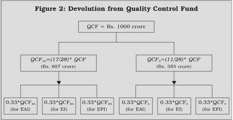 |
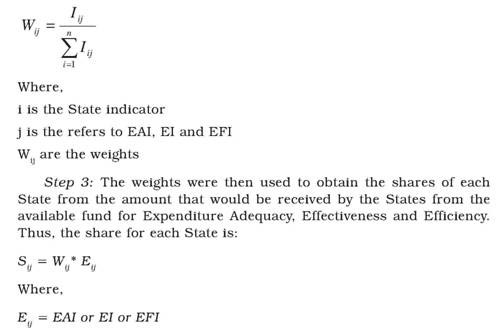 |
The shares of each State from the QCF that were obtained using the procedure outlined above and the rankings of the States have been tabulated in Tables 10A and 10B.
Goa is the clear gainer from among the non-special category States, followed by Tamil Nadu, Karnataka and Kerala. Bihar and Uttar Pradesh receive the smallest amounts from this fund. From among the special category States, the biggest gainer is Sikkim followed by Mizoram, while Assam and Jammu and Kashmir are the worst performers.
We did check on the sensitivity of the shares received by the States by varying the weights assigned to Expenditure Adequacy, Effectiveness and Efficiency. Two alternate scenarios were created:
Table 10A: State-wise Shares from Quality Control Fund (Non-Special Category States) |
QCF = Rs.l000crore
QCFns = Rs.607 crore |
(In Rupees crore) |
|
Expenditure
Adequacy
(EAI) |
Effectiv
eness (EI) |
Efficiency
(EFI) |
Total Allocation of State from QCFns |
Share of
State
(Per cent) |
Rank |
QCFns
(Criteria-wise) |
202.33 |
202.33 |
202.33 |
607.00 |
|
|
Andhra Pradesh |
11.75 |
9.44 |
9.22 |
30.41 |
5.01 |
10 |
Bihar |
9.41 |
3.53 |
8.42 |
21.36 |
3.52 |
17 |
Chhattisgarh |
11.04 |
8.37 |
20.56 |
39.97 |
6.58 |
6 |
Goa |
24.03 |
14.61 |
23.16 |
61.79 |
10.18 |
1 |
Gujarat |
11.72 |
15.85 |
9.45 |
37.02 |
6.10 |
9 |
Haryana |
12.81 |
5.17 |
9.68 |
27.65 |
4.56 |
12 |
Jharkhand |
10.78 |
14.85 |
16.95 |
42.59 |
7.02 |
5 |
Karnataka |
11.96 |
25.21 |
9.36 |
46.53 |
7.67 |
3 |
Kerala |
11.82 |
23.48 |
8.60 |
43.91 |
7.23 |
4 |
Madhya Pradesh |
10.29 |
3.97 |
8.99 |
23.26 |
3.83 |
15 |
Maharashtra |
12.39 |
5.71 |
9.06 |
27.17 |
4.48 |
14 |
Orissa |
10.30 |
6.46 |
20.74 |
37.51 |
6.18 |
7 |
Punjab |
11.81 |
7.04 |
8.43 |
27.27 |
4.49 |
13 |
Rajasthan |
10.98 |
16.93 |
9.17 |
37.07 |
6.11 |
8 |
Tamil Nadu |
11.92 |
32.02 |
9.60 |
53.53 |
8.82 |
2 |
Uttar Pradesh |
9.85 |
3.72 |
8.43 |
22.00 |
3.62 |
16 |
West Bengal |
9.53 |
6.01 |
12.56 |
28.10 |
4.63 |
11 |
Scenario 1: 20% (EAI) 40% (EI) 40% (EFI)
Scenario 2: 50% (EAI) 25% (EI) 25% (EFI)
The first scenario was intended to give greater weight to output and efficiency, which are intended to capture the impact of spending, and the second scenario was intended to give maximum weight to expenditure adequacy, as this is the first stage of improving on expenditure quality. The relative rankings of the States in these alternate scenarios are presented in Tables 11A and 11B.
Table 10B: State-wise Shares from Quality Control Fund (Special Category States) |
QCFs = Rs.393 crore |
(In Rupees crore) |
|
Expenditure
Adequacy
(EAI) |
Effectiveness (EI) |
Efficiency (EFI) |
Total Allocation of State from QCFns |
Share of
State
(Per cent) |
Rank |
QCFs
(Criteria-wise) |
131.00 |
131.00 |
131.00 |
393.00 |
|
|
Arunachal Pradesh |
17.11 |
10.28 |
29.19 |
56.59 |
14.40 |
3 |
Assam |
3.26 |
2.31 |
8.88 |
14.45 |
3.68 |
11 |
Himachal Pradesh |
5.12 |
10.78 |
10.41 |
26.31 |
6.70 |
6 |
Jammu and |
5.60 |
14.08 |
4.50 |
24.18 |
6.15 |
10 |
Kashmir |
|
|
|
|
|
|
Manipur |
4.97 |
11.00 |
4.10 |
20.07 |
5.11 |
7 |
Meghalaya |
4.22 |
2.29 |
10.72 |
17.23 |
4.39 |
4 |
Mizoram |
40.09 |
11.49 |
24.43 |
76.01 |
19.35 |
2 |
Nagaland |
4.90 |
1.60 |
1.66 |
8.16 |
2.08 |
5 |
Sikkim |
37.30 |
32.49 |
30.96 |
100.76 |
25.65 |
1 |
Tripura |
4.45 |
26.08 |
2.44 |
32.98 |
8.39 |
8 |
Uttarakhand |
3.91 |
8.55 |
3.66 |
16.12 |
4.10 |
9 |
We find the relative rankings to be completely unchanged in Scenario 1 where we give a relatively higher weight to Effectiveness and Efficiency. Only in scenario 2 where 50% weight is assigned to Expenditure Adequacy we find an improvement in the relative rankings of some States. Maharashtra, Haryana and Gujarat show an improved ranking in scenario 2 because as we had noted previously these States have fared well on the Expenditure Adequacy Index. The alternate scenarios for non-special
category States show no change at all in the relative ranks. Thus, the relative positions of States appear to be fairly robust to any change in weights for the three indices.
Table 11A: Alternate Scenarios: Non-Special Category States |
State |
Equal Weights
(as reported in table
10A and B) |
20% (EAI) 40% (EI) 40% (EFI) |
50% (EAI) 25% (EI) 25% (EFI) |
Rs. crore |
Rank |
Rs. crore |
Rank |
Rs. crore |
Rank |
Andhra Pradesh |
30.41 |
10 |
29.44 |
10 |
31.62 |
10 |
Bihar |
21.36 |
17 |
19.98 |
17 |
23.08 |
17 |
Chhattisgarh |
39.97 |
6 |
41.35 |
6 |
38.26 |
6 |
Goa |
61.79 |
1 |
59.73 |
1 |
64.36 |
1 |
Gujarat |
37.02 |
9 |
37.39 |
9 |
36.56 |
7 |
Haryana |
27.65 |
12 |
25.50 |
13 |
30.34 |
11 |
Jharkhand |
42.59 |
5 |
44.63 |
5 |
40.03 |
5 |
Karnataka |
46.53 |
3 |
48.66 |
3 |
43.87 |
3 |
Kerala |
43.91 |
4 |
45.60 |
4 |
41.80 |
4 |
Madhya Pradesh |
23.26 |
15 |
21.73 |
15 |
25.16 |
15 |
Maharashtra |
27.17 |
14 |
25.17 |
14 |
29.67 |
12 |
Orissa |
37.51 |
7 |
38.83 |
7 |
35.86 |
9 |
Punjab |
27.27 |
13 |
25.64 |
12 |
29.31 |
13 |
Rajasthan |
37.07 |
8 |
37.90 |
8 |
36.04 |
8 |
Tamil Nadu |
53.53 |
2 |
57.09 |
2 |
49.09 |
2 |
Uttar Pradesh |
22.00 |
16 |
20.49 |
16 |
23.88 |
16 |
West Bengal |
28.10 |
11 |
28.00 |
11 |
28.22 |
14 |
Table 11B: Alternate Scenarios: Special Category States |
State |
Equal Weights
(as reported in table
10A and B) |
20% (EAI) 40% (EI) 40% (EFI) |
50% (EAI) 25%
(EI) 25% (EFI) |
Rs. crore |
Rank |
Rs. crore |
Rank |
Rs. crore |
Rank |
Arunachal Pradesh |
56.59 |
3 |
57.64 |
3 |
55.28 |
3 |
Assam |
14.45 |
10 |
15.38 |
10 |
13.29 |
10 |
Himachal Pradesh |
26.45 |
5 |
28.50 |
5 |
23.57 |
5 |
Jammu and Kashmir |
24.18 |
6 |
25.65 |
6 |
22.33 |
6 |
Manipur |
20.07 |
7 |
21.11 |
7 |
18.78 |
7 |
Meghalaya |
17.23 |
8 |
18.15 |
8 |
16.09 |
8 |
Mizoram |
76.01 |
2 |
67.16 |
2 |
87.08 |
2 |
Nagaland |
8.16 |
11 |
6.85 |
11 |
9.79 |
11 |
Sikkim |
100.76 |
1 |
98.52 |
1 |
103.54 |
1 |
Tripura |
32.98 |
4 |
36.90 |
4 |
28.07 |
4 |
Uttarakhand |
16.12 |
9 |
17.00 |
9 |
15.03 |
9 |
VII. Summary and Conclusion
The present study has sought to introduce, conceptualise and operationalise a scheme for integrating the ‘quality’ dimension of public spending into the devolution scheme of intergovernmental transfers by the Finance Commission.
The Twelfth Finance Commission mentioned the importance of outcome in expenditure management and made a beginning towards improving expenditure ‘quality’ by recommending special grants for education and health for certain States. The Thirteenth Finance Commission needs to carry this further especially since it has been given the mandate to incorporate expenditure ‘quality’ in its recommendations. We strongly urge the Thirteenth Finance Commission to reward the States for their performance on Expenditure Quality, tie the funds that the States receive from this incentive fund to spending on education and health and make a small beginning towards results-based approach by mandating that output targets be set for the funds received from the Quality Control Fund.
The operational part of the scheme being recommended is certainly open to some fine tuning in case of all the three Es of our Triple-E approach: (i) The definition of Public Goods when using the expenditure adequacy measure could be made more precise by using the Finance Accounts (lack of easy access to this data source for a few years prevented its use here); (ii) Some more innovative output measures could be experimented with to obtain performance indicators to gauge the effectiveness – also one could make this measure more comprehensive by including output indicators for basic amenities such as for water and housing; and (iii) The efficiency indices too could also be made more comprehensive. While all this fine tuning could improve our measure of expenditure ‘quality’, the central message of this study remains unchanged – a ‘Quality Control Fund’ should be created by the Finance Commission. Inter-se distribution from this would be a reward to the States for their performance in the context of expenditure quality. The funds received from this incentive fund should be tied to spending on education and health. It would be a major change of approach if the Finance Commission went a step further and mandated the States to set out some realistic output targets for the funds that they received from the Quality Control Fund. Even if resource constraints meant that the Finance Commission could set aside only a very small Quality Control Fund – it would be a big stride towards results-based output-oriented transfers and could herald a sea change in the very approach of budgeting and intergovernmental relations!
References
Ablo, Emmanuel, and Ritva Reinikka, 1998, Do Budgets Really Matter? Evidence from Public Spending on Education and Health in Uganda, World Bank Policy Research Working Paper No. 1926 (Washington: World Bank).
Afonso, A., L. Schuknecht and V. Tanzi (2003): Public Sector Efficiency: An International Comparison, ECB Working Paper no. 242.
Afonso, A., L. Schuknecht and V. Tanzi (2005): Public sector efficiency: An international comparison, Public Choice vol. 123, pp. 321-347.
Afonso, A. and St. Aubyn (2004): Non-Parametric Approaches to Education and Health: Expenditure Efficiency in OECD Countries, (Mimeo), ISEG/UTL-Technical University of Lisbon.
Andrews, M. (2005) : Performance Based Budgeting Reform: Progress, Problems and Pointers in Shah ed., Fiscal Management, World Bank.
Asian Development Bank (2001): What is Public Expenditure Management, The Governance Brief.
Atkinson, A.B. et al. (2005) Measurement of Government Output and Productivity for the National Accounts, Basingstoke: Palgrave.(http://www.statistics.gov.uk/about/data/methodology/specific/PublicSector/Atkinson/downloads/Atkinson_Report_Full.pdf).
Banker, R.D., A. Charnes and W.W. Cooper (1984): Some Models for Estimating Technical and Scale Efficiencies in Data Envelopment Analysis, Management Science, vol. 30 (9), pp. 1078-1092.
Brennan, G. and J.M. Buchanan (1980): The Power to Tax: Analytical Foundation of a Fiscal Constitution, Cambridge University Press, Cambridge.
Charnes, A., W.W. Cooper, and E. Rhodes (1978): Measuring the Efficiency of Decision Making Units, European Journal of Operational Research, vol.2, pp. 429-444.
Clements, (2002): “How Efficient is Education Spending in Europe?” European Review of Economics and Finance, 1(1), 3-26.
Diamond, J.(2006): Budget System Reform in Emerging Economies: The Challenges and theReform Agenda, Occasional Paper No. 245 (Washington: International Monetary Fund).
Garg, S.C. (2006): Transformation of Central Grants to States Growing Conditionality and Bypassing State Budgets, Economic and Political Weekly, December 2.
GOI, (1997): Government Subsidies in India, Discussion Paper.
Gupta and Verhoven (2001): “The Efficiency of Government Expenditure –Experiences from Africa”, Journal of Policy Modelling, 23, pp. 433-467.
Heller, P. (2005): Understanding Fiscal Space, IMF Policy Discussion Paper, PDP 05/4.
Heller, P. (2007): Fiscal Policy for Growth and Development: The Fiscal Space Debate, Paper presented at G-20 Workshop on Fiscal Policy: Fiscal Elements of Growth and Development, Istanbul.
Hoppner, F. and C. Kastrop (2005): The Role of “Quality of Public Finances” in the Context of the Reformed Stability and Growth Pact paper presented at Banca D’Italia Research Department Public Finance Workshop in Public Expenditure.
Jacobs, R., P.C. Smith and A. Street (2006): Measuring Efficiency in Health Care, Analytic Techniques and Health Policy, Cambridge University Press.
Jurgen Von Hagen (2005) in Shah (ed.), Fiscal Management, World Bank, USA.
Karnik, A.V. A.M. Pethe and D. Karmarkar (2001): Developing a Quantitative Framework for Determining Devolution of funds from the State Government to Local Bodies Final Report submitted to Maharashtra State Finance Commission, Government of Maharashtra, September, 2001.
Karnik, A.V. A.M. Pethe and D. Karmarkar (2006): Developing a Quantitative Framework for Determining Devolution of funds from the State Government to Local Bodies in Niraja Jayal, Amit Prakash and Pradeep Sharma (eds) Local Governance in India: Decentralization and Beyond, Oxford University Press, New Delhi.
Lalvani, M. (2008): Budget 2008-09: Demonstrating a ‘New Political Budget Cycle’, Economic and Political Weekly.
Lonti, Z. and M. Woods (2008) Towards Government at a Glance: Identification of Core Data and Issues related to Public Sector Efficiency, OECD Working Paper on Public Governance no. 7 OECD Publishing.
Manning, Nick, D.J. Kraan and J. Malinska (2006). “How and Why Should Government Activity Be Measured in Government at a Glance?” OECD: Paris.
McCarten (2000) Multi-Tiered Governments and Hard/Soft Budget Constraints: The Case of India http://www1.worldbank.org/wbiep/deCentralization/saslib/McCarten.pdf.
Miles, D., G. Myles and I. Preston, 2003: The Economics of Public Spending, Oxford University Press, New York.
Mueller, D. (2003): Public Choice III, Cambridge University Press.
Paul, S., S. Balakrishnan, K. Gopakumar, S. Sekhar, M. Vivekananda (2004): State of India’s Public Services: Benchmarks for the States, Economic and Political Weekly, February 28.
Pedraja-Chpparo F.,J. Jimenez and P. Smith (2005): Assessing Public Sector Efficiency: Issues and Methodologies, paper presented at Banca D’Italia Research Department Public Finance Workshop in Public Expenditure.
Prayas Energy Group (2008): Awareness and Action for Better Electricity Supply: An Agenda for the Community, Pune.
Reinikka, Ritva, and Jakob Svensson, 2004, “Local Capture: Evidence from a Central Government Transfer Program in Uganda,” Quarterly Journal of Economics, Vol. 119, No. 2, pp. 679–705.
Reserve Bank of India, “State Finances – A Study of Budgets”, various issues.
Schick, Allen, 1997, Modern Budgeting (Paris: Organisation for Economic Co-operation and Development).
Seabright, P. (1996): Accountability and Decentralisation in Government: an Incomplete Contracts Model”, European Economic Review, 1996.
Shah, A. (2000): Governing for Results in a Globalized and Localized World, Paper presented at the International Conference on Federalism, Monterry, Mexico, March.
Shah, A. (2007a): A Practitioner’s Guide to Intergovernmental Fiscal Transfers in Intergovernmental Fiscal Transfers: Principles and Practice ed., R. Boadway and A. Shah, The World Bank.
Shah, A. (2007b): A Framework Evaluating Alternative Institutional Arrangements for Fiscal Equalization Transfers in Fiscal Equalization: Challenges in The Design of Intergovernmental Transfers ed. Jorge Marinez-Vazquez and Bob Searle, Springer, USA.
Srivastava, D.K. et al. (2003): Budgetary Subsidies in India: Subsidising Social and Economic Services, NIPFP.
St. Aubyn (2002): Evaluating Efficiency in the Portuguese Health and Education Sectors, paper presented to the conference “Desenvolvimento Económico Português no Espaço Europeu: Determinantes e Políticas”, Banco de Portugal, May, Fundação Calouste Gulbenkian, Lisbon.
St. Aubyn (2003): “Evaluating efficiency in the Portuguese Education Sector”, Economia, (forthcoming).
Tanzi, V. , 2000, “Rationalizing the Government Budget: Or Why Fiscal Policy Is So Difficult,” in Economic Policy Reform: The Second Stage, ed. by Anne O. Krueger (Chicago: University of Chicago Press), pp. 435–52.
Tullock, G. (1959): Problems of majority voting. Journal of Political Economy vol. 67, pp. 571–579.
Van Dooren, W. et. al. (2007): Institutional Drivers Of Efficiency In The Public Sector Public Governance no. GOV/PGC(2007) 16/ANN, OECD publishing http://www.oecd.org/dataoecd/42/38/40305170.pdf.
Von Hagen, J. (2002): Fiscal Rules, Fiscal Institutions, and Fiscal Performance, The Economic and Social Review, Vol. 33, No. 3, Winter, 2002, pp. 263-284
Von Hagen, J. and I. Harden (1996): Budget Processes and Commitment to Fiscal Discipline, IMF working paper.
Weingast, B., K. Shepsle and C. Johnsen (1981): The Political Economy of Benefits and Costs: A Neoclassical Approach to Distributive Politics, Journal of Political Economy, vol. 89, no..4 pp.642-664.
World Bank (2004): World Development Report: Making Services Work for the Poor, World Bank.
World Bank (2006): Reforming Public Services in India: Drawing Lessons from Success, A World Bank Report, World Bank.
Ye, Xiao, and Sudharshan Canagarajah (2002): Efficiency of Public Expenditure Distribution and Beyond: A Report on Ghana’s 2000 Public Expenditure Tracking Survey in the Sectors of Primary Health and Education, Africa Region Working Paper Series No. 31 (Washington: World Bank).
Appendix
Appendix A |
Detailed Composition of Major Heads which define Public and Merit Goods |
Public Goods |
(1) |
Medical and Public Health: This broad expenditure category (as available in State Finances, RBI) includes: |
|
(i) |
Urban Health Services-Allopathy which comprises of Employee State Insurance, Central Government Health Scheme, Hospitals and Dispensaries; |
|
(ii) |
Urban Health Services – other systems of Medicine; |
|
(iii) |
Rural Health Services – Allopathy which includes Sub-Centres, Primary Health Centres, and Community Health Centres; |
|
(iv) |
Rural Health Services – other systems of Medicine; |
|
(v) |
Medical Education, Training and Research; |
|
(vi) |
Public Health including Public Health Laboratories, Public Health Education, training, prevention of food adulteration; and |
|
(vii) |
General category including health statistics and evaluation. |
(2) |
Soil and Water Conservation: This category of expenditure includes the following categories: |
|
(i) |
Soil survey and testing; |
|
(ii) |
Soil conservation; |
|
(iii) |
Land reclamation; |
|
(iv) |
Extension and training. |
(3) |
Forestry and Wild Life: This comprises of: |
|
(i) |
Forestry including education and training, research, forest conservation; |
|
(ii) |
Environmental Forestry and Wild Life including wild life preservation, zoological park, public gardens; |
|
(iii) |
Afforestation and Ecology. |
Appendix A (Contd.) |
Detailed Composition of Major Heads which define Public and Merit Goods |
(4) |
Agricultural Research and Foundation: This includes |
|
(i) |
Major Irrigation; |
|
(ii) |
Medium Irrigation (Commercial and Non-Commercial) both of which includes |
|
|
(a) Machinery and equipment, direction and administration and |
|
|
(b) General including Research, training, survey and investigation. |
(5) |
Power |
(6) |
Roads and Bridges |
(7) |
Police |
Merit Goods |
(1) |
Education, Sports, Art and Culture: More specifically this broad expenditure category comprises of: |
|
(i) |
Elementary Education; |
|
(ii) |
Secondary Education; |
|
(iii) |
University and Higher Education; |
|
(iv) |
Adult Education; |
|
(v) |
Language Development; |
|
(vi) |
General. |
(2) |
Family Welfare: This expenditure head would clearly qualify as a merit good as the Government adopts a paternalistic role and advises people. It includes |
|
(i) |
Training; |
|
(ii) |
Research and Evaluation; |
|
(iii) |
Rural Welfare Services; |
Appendix A (Contd.) |
Detailed Composition of Major Heads which define Public and Merit Goods |
|
(iv) |
Urban Welfare Services; |
|
(v) |
Maternity and Child Health. |
(3) |
Water Supply and Sanitation: This broad expenditure category comprises: |
|
(i) |
Water Supply including Rural and Urban water supply programs; |
|
(ii) |
Sewerage and Sanitation, which includes |
|
|
(a) Training, Research, Survey and Investigation, |
|
|
(b) Machinery and Equipments, prevention of air and water sanitation. |
(4) |
Welfare of SC, ST and OBC: It comprises of: |
|
a. |
Welfare of SC and of ST, |
|
b. |
Welfare of Backward Classes; and |
|
c. |
General expenditures. |
Apart from education, housing, administration, this includes expenditure on Health for SC, ST and Tribals, which could be classified as public goods. |
(5) |
Labour and Labour Welfare: It includes three Sub-Major Heads |
|
(i) |
Labour including minor heads like industrial relations, labour welfare, education; |
|
(ii) |
Employment Service; and |
|
(iii) |
Training including minor heads like research and statistics, working conditions and safety, training of craftsmen and supervisors. |
(6) |
Social Security and Welfare: It includes three sub-major heads, viz., |
|
(i) |
Rehabilitation, which includes rehab of repatriates, displaced persons; |
|
(ii) |
Social welfare, including child welfare, women’s welfare, welfare of handicapped, welfare of aged, infirm and destitute; |
Appendix A (Concld.) |
Detailed Composition of Major Heads which define Public and Merit Goods |
|
(iii) |
National Social Assistance Program, including Old Age Pensions scheme, Family Benefit Scheme, Maternity Benefit Scheme; and |
|
(iv) |
Other Social Security and Welfare Programs, including Government employee insurance schemes, pensions under social security schemes. |
(7) |
Nutrition: This comprises three sub-Major heads; |
|
(i) |
Production of Nutritious Foods and Beverages; |
|
(ii) |
Distribution of Nutritious Foods and Beverages; including Special Nutrients Programs and Mid-day Meals; and |
|
(iii) |
General including Research and Development, Diet Surveys and Nutrition Planning, Nutrition education, statistics and evaluation. Some of the minor heads like research and education would typically classify as pure public goods. |
(8) |
Relief on Account of Natural Calamities: This includes the following: |
|
(i) |
Drought; |
|
(ii) |
Floods and Cyclones; |
|
(iii) |
Famine Relief Fund; |
|
(iv) |
Calamity Relief Fund. The minor heads under each includes Public Health, Veterinary Care, Drinking water, nutrition, assistance to farmers for repairs, damages etc. |
Appendix B |
Table B1: Fiscal Responsibility Legislation of States-Month and Year of Enactment |
State |
Month / Year of Enactment |
State |
Month / Year of Enactment |
1 |
Andhra Pradesh |
Jun-05 |
15 |
Maharashtra |
Apr-05 |
2 |
Arunachal Pradesh |
Mar-06 |
16 |
Manipur |
Aug-05 |
3 |
Assam |
Sep -05 |
17 |
Meghalaya |
Mar-06 |
4 |
Bihar |
Apr-06 |
18 |
Mizoram |
Oct-06 |
5 |
Chhattisgarh |
Sep-05 |
19 |
Nagaland |
Aug-05 |
6 |
Goa |
May-06 |
20 |
Orissa |
Jun-05 |
7 |
Gujarat |
Mar-05 |
21 |
Punjab |
Oct-03 |
8 |
Haryana |
Jul-05 |
22 |
Rajasthan |
May-05 |
9 |
Himachal Pradesh |
Apr-05 |
23 |
Sikkim |
No |
10 |
Jammu and Kashmir |
Aug-06 |
24 |
Tamil Nadu |
May-0o |
11 |
Jharkhand |
May-07 |
25 |
Tripura |
Jun-05 |
12 |
Karnataka |
Sep-02 |
26 |
Uttarakhand |
Oct-05 |
13 |
Kerala |
Aug-03 |
27 |
Uttar Pradesh |
Feb-04 |
14 |
Madhya Pradesh |
May-05 |
28 |
West Bengal |
No |
Note: Sikkim and West Bengal have not enacted FRL. |
Appendix B (Contd.) |
Table B2: Components of Developmental Expenditure of States
(as Per Cent of GDP) |
Item |
1990-95 |
1995-00 |
2000-05 |
2005-06 |
2006-07 |
2007-08 |
(Average) |
(RE) |
(BE) |
1. |
Developmental Expenditure (Revenue & Capital) (A + B) |
9.84 |
8.78 |
8.89 |
8.83 |
9.76 |
9.63 |
|
A. |
Social Services (a to l) |
4.84 |
4.71 |
4.76 |
4.54 |
5.02 |
4.97 |
|
|
(a) |
Education, Sports, Art and Culture |
2.60 |
2.53 |
2.51 |
2.23 |
2.35 |
2.28 |
|
|
(b) |
Medical and Public Health |
0.80 |
0.61 |
0.57 |
0.54 |
0.60 |
0.58 |
|
|
(c) |
Family Welfare |
- |
0.12 |
0.10 |
0.08 |
0.09 |
0.08 |
|
|
(d) |
Water Supply and Sanitation |
0.36 |
0.36 |
0.38 |
0.38 |
0.39 |
0.39 |
|
|
(e) |
Housing |
0.09 |
0.09 |
0.08 |
0.08 |
0.11 |
0.12 |
|
|
(f) |
Urban Development |
0.11 |
0.13 |
0.18 |
0.20 |
0.33 |
0.42 |
|
|
(g) |
Welfare of SCs, STs and OBCs |
0.33 |
0.31 |
0.31 |
0.33 |
0.37 |
0.38 |
|
|
(h) |
Labour and Labour Welfare |
0.07 |
0.06 |
0.05 |
0.05 |
0.06 |
0.05 |
|
|
(i) |
Social Security and Welfare |
0.23 |
0.20 |
0.25 |
0.26 |
0.34 |
0.37 |
|
|
(j) |
Nutrition |
0.09 |
0.13 |
0.10 |
0.11 |
0.13 |
0.12 |
|
|
(k) |
Expenditure on Natural Calamities |
0.13 |
0.14 |
0.18 |
0.24 |
0.19 |
0.11 |
|
|
(l) |
Others |
0.04 |
0.04 |
0.05 |
0.06 |
0.07 |
0.07 |
|
B. |
Economic Services (a to i) |
5.01 |
4.07 |
4.12 |
4.28 |
4.74 |
4.66 |
|
|
(a) |
Agriculture and Allied Activities |
1.13 |
0.86 |
0.75 |
0.63 |
0.73 |
0.70 |
|
|
(b) |
Rural Development |
0.82 |
0.58 |
0.56 |
0.60 |
0.67 |
0.66 |
|
|
(c) |
Special Area Programmes |
0.09 |
0.08 |
0.06 |
0.06 |
0.09 |
0.07 |
|
|
(d) |
Irrigation and Flood Control |
1.22 |
1.08 |
0.95 |
1.05 |
1.16 |
1.14 |
|
|
(e) |
Energy |
0.61 |
0.56 |
0.93 |
0.89 |
0.86 |
0.83 |
|
|
(f) |
Industry and Minerals |
0.27 |
0.18 |
0.13 |
0.13 |
0.14 |
0.15 |
|
|
(g) |
Transport and Communications |
0.63 |
0.57 |
0.56 |
0.70 |
0.84 |
0.84 |
|
|
(h) |
Science, Technology and Environment |
0.01 |
0.01 |
0.01 |
0.01 |
0.01 |
0.01 |
|
|
(i) |
General Economic Services |
0.24 |
0.16 |
0.18 |
0.21 |
0.23 |
0.26 |
2. |
Loans and Advances by State Governments |
0.87 |
0.57 |
0.53 |
0.39 |
0.35 |
0.33 |
Total Developmental Expenditure (1 + 2) |
10.72 |
9.36 |
9.42 |
9.22 |
10.11 |
9.96 |
RE: Revised Estimates.BE: Budget Estimates.
Source: State Finances, RBI, various issues. |
Appendix B (Contd.) |
Table B3: Guarantees of State Governments as per cent of Revenue Receipts |
(As at end-March 2006) |
(Per cent) |
State |
Guarantees/Revenue Receipts |
1. |
Andhra Pradesh |
49.9 |
2. |
Assam |
10.1 |
3. |
Bihar |
3.3 |
4. |
Gujarat |
56.2 |
5. |
Haryana |
40.2 |
6. |
Himachal Pradesh |
105.0 |
7. |
Jammu and Kashmir |
N.A. |
8. |
Karnataka |
29.6 |
9. |
Kerala |
78.0 |
10. |
Madhya Pradesh |
66.5 |
11. |
Maharashtra |
122.8 |
12. |
Orissa |
24.8 |
13. |
Punjab |
54.4 |
14. |
Rajasthan |
62.9 |
15. |
Tamil Nadu |
18.6 |
16. |
Uttar Pradesh |
25.2 |
17. |
West Bengal |
57.0 |
Total (Per cent of Revenue Receipts) |
45.7 |
Note: Data are available for only 17 States.
Source: State Finances 2007-08, RBI. |
Appendix B (Contd.) |
Table B4: Virtuous Fiscal Space (As Per cent of Revenue Receipts) |
|
Centre |
States |
Non-Spl. Category States |
Spl. Category States |
2001-02 |
67.43 |
39.83 |
39.96 |
42.87 |
2002-03 |
67.43 |
42.64 |
39.46 |
42.76 |
2003-04 |
64.54 |
39.76 |
42.83 |
41.23 |
2004-05 |
59.32 |
40.58 |
38.97 |
45.90 |
2005-06 |
63.74 |
39.63 |
39.69 |
47.26 |
2006-07 |
63.26 |
41.39 |
40.23 |
34.79 |
Appendix B (Contd.) |
Table B5: Expenditure Per Capita Special and Non-Special Category States |
(Rs.) |
State |
Public Goods |
Merit Goods |
Non-Special Category States |
Andhra Pradesh |
1706.37 |
1282.92 |
Bihar |
480.94 |
637.83 |
Chhattisgarh |
1145.13 |
1208.38 |
Goa |
6077.74 |
4109.65 |
Gujarat |
1594.41 |
1317.83 |
Haryana |
1934.42 |
1568.37 |
Jharkhand |
1003.49 |
1146.16 |
Karnataka |
1710.90 |
1361.20 |
Kerala |
1039.69 |
1529.87 |
Madhya Pradesh |
1111.73 |
870.23 |
Maharashtra |
1470.61 |
1592.88 |
Orissa |
652.21 |
1045.99 |
Punjab |
1861.36 |
1239.14 |
Rajasthan |
970.89 |
1239.33 |
Tamil Nadu |
1042.89 |
1559.80 |
Uttar Pradesh |
902.21 |
718.98 |
West Bengal |
425.77 |
726.12 |
AVERAGE |
1478.28 |
1362.04 |
Special Category States |
Arunachal Pradesh |
4946.80 |
4256.98 |
Assam |
964.59 |
1442.85 |
Himachal Pradesh |
2584.74 |
3101.47 |
Jammu and Kashmir |
3553.99 |
1961.38 |
Manipur |
2885.49 |
2538.51 |
Meghalaya |
2219.13 |
2221.53 |
Mizoram |
5528.04 |
5143.14 |
Nagaland |
3088.59 |
1986.50 |
Sikkim |
5232.19 |
5934.80 |
Tripura |
2258.87 |
2562.38 |
Uttarakhand |
1837.53 |
2068.83 |
AVERAGE |
3190.90 |
3019.85 |
Public Goods: Medical and Public Health, Soil and Water Conservation, Forestry and Wild Life, Agricultural Research and Foundation, Power, Roads and Bridges, Police.
Merit Goods: Education, Sports, Art and Culture, Family Welfare, Water Supply and Sanitation, Welfare of SC, ST and OBC, Labour and Labour Welfare, Social Security and Welfare, Nutrition, Relief on Account of Natural Calamities.
Source: State Finances, RBI various issues. |
Appendix B (Contd.)
|
B6: Data for Effectiveness Index |
State |
T&D losses
(as % of
availability) |
Incidence of
cognizable
crimes |
Shortfall in PHC/CHC/SUBC as % of required
as per norms |
Doctor per PHC |
Gross enrolment
ratio in secondary
education (IX-XII)
(enrolment/
population of relevant age group) |
Pupil
Teacher
Ratio in
high & post
basic schools |
|
(Per cent) |
(nos.) |
(Per cent) |
(nos.) |
(Per cent) |
(nos.) |
Non-Special Category States |
Andhra Pradesh |
23.76 |
173909 |
4.74 |
1.40 |
47.66 |
33 |
Bihar |
35.87 |
100665 |
41.51 |
0.98 |
32.23 |
55 |
Chhattisgarh |
26.68 |
45177 |
3.75 |
2.23 |
37.3 |
38 |
Goa |
35.15 |
2204 |
1.85 |
2.79 |
57.82 |
24 |
Gujarat |
30.29 |
120972 |
1.37 |
0.85 |
38.64 |
34 |
Haryana |
32.00 |
50509 |
19.48 |
1.06 |
43.6 |
27 |
Jharkhand |
21.02 |
36364 |
26.09 |
7.07 |
14.8 |
54 |
Karnataka |
22.12 |
117710 |
0.54 |
1.22 |
46.4 |
18 |
Kerala |
22.16 |
105255 |
1.57 |
1.27 |
60.15 |
27 |
Madhya Pradesh |
41.27 |
194711 |
17.57 |
0.70 |
35.72 |
32 |
Maharashtra |
32.39 |
191788 |
13.48 |
0.66 |
55.6 |
35 |
Orissa |
33.24 |
52792 |
16.20 |
1.06 |
43.43 |
22 |
Punjab |
25.12 |
32068 |
10.83 |
0.72 |
39.6 |
28 |
Rajasthan |
44.77 |
141992 |
0.55 |
0.77 |
33.06 |
27 |
Tamil Nadu |
19.18 |
148972 |
1.50 |
2.03 |
62.08 |
29 |
Uttar Pradesh |
34.93 |
127001 |
22.82 |
0.62 |
36.32 |
61 |
West Bengal |
24.70 |
68052 |
20.34 |
0.88 |
31.39 |
63 |
Special Category States |
Arunachal Pradesh |
30.86 |
2294 |
0.00 |
0.92 |
42.37 |
28 |
Assam |
51.07 |
43673 |
5.28 |
1.00 |
32.23 |
20 |
Himachal Pradesh |
15.35 |
13093 |
0.00 |
1.06 |
131.26 |
26 |
Jammu & Kashmir |
40.36 |
20787 |
0.00 |
1.72 |
35.38 |
14 |
Manipur |
70.61 |
2884 |
0.00 |
1.33 |
48.61 |
24 |
Meghalaya |
26.23 |
1935 |
27.64 |
1.05 |
33.27 |
24 |
Mizoram |
63.67 |
2073 |
0.00 |
0.61 |
44.67 |
12 |
Nagaland |
48.26 |
1103 |
21.73 |
0.63 |
21.28 |
23 |
Sikkim |
43.75 |
703 |
0.00 |
2.00 |
33.3 |
11 |
Tripura |
49.53 |
3940 |
21.17 |
2.08 |
38.86 |
25 |
Uttaranchal |
37.21 |
8412 |
0.26 |
0.82 |
58.03 |
18 |
Source: www.indiastat.com |
Appendix B (Concld.) |
Table B7: Efficiency Parameters from DEA (Constant returns to scale) |
State |
Crime |
Secondary Education |
Rural Health |
Power |
Non-Special Category States |
Andhra Pradesh |
0.21 |
0.047 |
0.436 |
0.072 |
Bihar |
0.181 |
0.04 |
0.312 |
0.002 |
Chhattisgarh |
1 |
0.178 |
1 |
0.172 |
Goa |
1 |
1 |
1 |
0.003 |
Gujarat |
0.46 |
0.058 |
0.24 |
0.063 |
Haryana |
0.32 |
0.169 |
0.423 |
0.018 |
Jharkhand |
0.163 |
0.083 |
1 |
0.039 |
Karnataka |
0.207 |
0.099 |
0.455 |
0.039 |
Kerala |
0.223 |
0.085 |
0.243 |
0.107 |
Madhya Pradesh |
0.304 |
0.083 |
0.327 |
0.026 |
Maharashtra |
0.402 |
0.029 |
0.196 |
0.118 |
Orissa |
0.499 |
0.193 |
0.776 |
1 |
Punjab |
0.232 |
0.134 |
0.183 |
0.04 |
Rajasthan |
0.295 |
0.068 |
0.372 |
0.05 |
Tamil Nadu |
0.264 |
0.063 |
0.453 |
0.111 |
Uttar Pradesh |
0.219 |
0.037 |
0.282 |
0.015 |
West Bengal |
0.496 |
0.031 |
0.21 |
0.637 |
AVERAGE |
0.380882 |
0.141 |
0.465176 |
0.147765 |
Special Category States |
Arunachal Pradesh |
0.687 |
0.99 |
1 |
0.694 |
Assam |
0.243 |
0.067 |
1 |
0.172 |
Himachal Pradesh |
0.828 |
0.651 |
1 |
0.629 |
Jammu and Kashmir |
0.563 |
0.202 |
0.945 |
0.044 |
Manipur |
0.625 |
0.69 |
0.927 |
0.148 |
Meghalaya |
1 |
0.628 |
0.968 |
0.901 |
Mizoram |
0.857 |
1 |
0.597 |
0.252 |
Nagaland |
0.393 |
0.421 |
0.699 |
0.407 |
Sikkim |
1 |
1 |
0.744 |
1 |
Tripura |
0.748 |
0.393 |
0.799 |
0.437 |
Uttarakhand |
0.31 |
0.264 |
0.657 |
1 |
AVERAGE |
0.66 |
0.57 |
0.85 |
0.52 |
Source: www.indiastat.com and State Finances, RBI, various issues. |
* Mala Lalvani is a Professor at the Department of Economics, University of Mumbai; Kumudini Hajra is Director, Division of State and Local Finances, Department of Economic Analysis and Policy (DEAP), Reserve Bank of India (RBI) and Brijesh Pazhayathodi is Research Officer, Division of Central Finances, DEAP, RBI.
1 We would like to thank Prof. Indira Rajaraman for drawing our attention to this at a meeting organised by the Maharashtra Economic Development Council (MEDC),
2 We consider expenditure on rural public health for the DEA exercise alone.
3 Other measures of obtaining efficiency measures or improved techniques could be experimented with. Currently as a first stage the freely available Data Envelopment Analysis Programme (DEAP) software has been employed. We would like to thank Dr. Abhiman Das, RBI for some crucial suggestions and for cautioning us about the care that needs to be exercised when using DEA and DEAP software. Also, advice from Dr. Uma Swaminathan, Department of Economics, University of Mumbai in gratefully acknowledged.
4 [(17/28)*1000] = Rs.607 crore for non-special category States and [(11/28)*1000] = Rs.393 crore for special category States. Please note that this scheme of bifuracation of the divisible pool is merely illustrative. |
 IST,
IST,