 IST,
IST,


Market Returns and Flows to Debt Mutual Funds
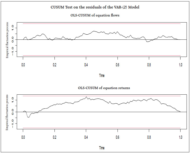
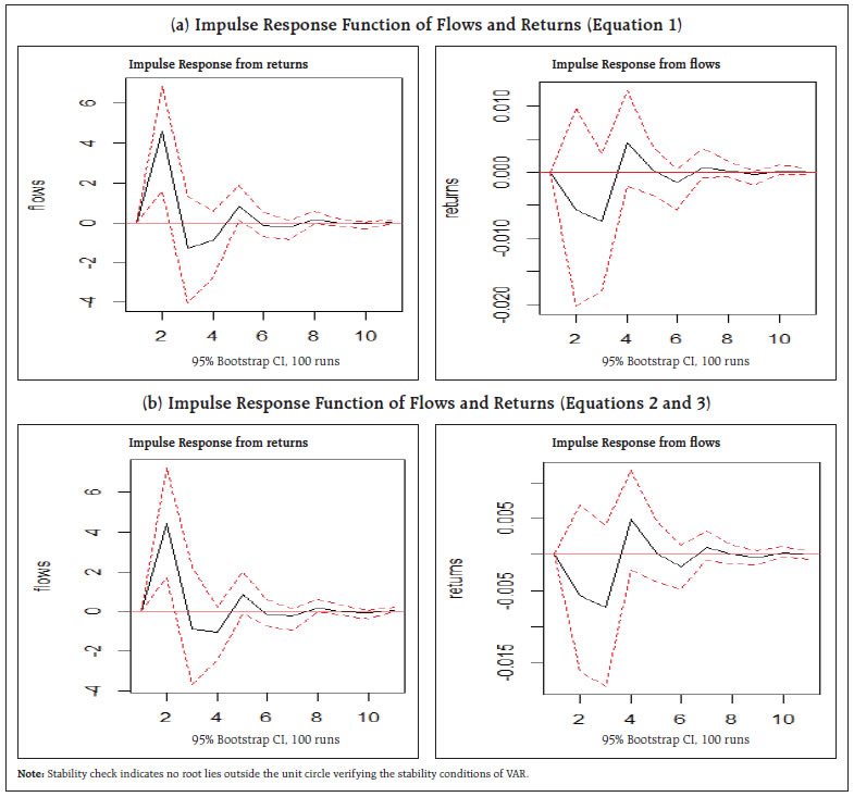
by Dr. Mayank Gupta^, Satyam Kumar^, The scale of debt-oriented mutual funds (MFs) in India has expanded over the years. The study examines drivers of flows to debt mutual funds. It investigates the relationship between net flows to debt MFs and return on debt MFs. We proxy debt MF returns by constructing an index using CRISIL benchmark indices. Further, the relationship between flows and returns on debt MFs is analysed in the presence of various market fundamentals. The study finds that returns cause flows but not vice-versa. Introduction There has been tremendous growth in the volume of debt securities in India. A significant part of the evolution of this market-led financial intermediation system has been supported by the debt-oriented MFs, which invest in debt securities. These debt-oriented MFs subscribe to short-tenor and long-tenor securities of Government and corporates, viz., T-bills, central government securities, state development loans (SDLs), commercial papers (CPs), certificates of deposit (CDs) and corporate bonds. Further, they are also active participants in Tri-party repo (TREPS) and market repo segments, predominantly on the lending side. Although return from equity mutual funds has been generally higher in the past, debt mutual funds have created a niche for themselves as certain investors try to avoid uncertainty and volatility in stock market. Besides, a stable and regular income motivates investors to prefer debt MFs. However, credit risk or risk of default is present as the issuer may default on interest or principal payments. Against this background, the study has attempted to understand the relationship between net flows to debt MFs and returns on debt MFs i.e., whether flows impact returns and/or returns impact flows in India. The overall return on debt MFs is not readily available, therefore, it is arrived at by constructing an index using monthly data on CRISIL benchmark indices against which the performance of debt mutual fund schemes are tracked. Further, the study estimates this relationship in the presence of market fundamentals by incorporating information on credit spreads, output/ state of the economy, rate of return on competitive savings instrument, liquidity and inflation rate. The rest of the article is organised as follows. Section II discusses stylised facts on debt MFs. Section III discusses determinants of flows to debt MFs. Section IV covers the analysis of relationship between net flows and return on debt MFs. Lastly, section V reports the concluding observations. Rise of Debt Securities and Debt Mutual Fund Industry The past decade has seen tremendous growth in the debt securities in India (Chart 1a). The share of debt securities in debt financing of corporates has also increased (Chart 1b). There are many advantages of having diversified financing mechanisms, viz., efficient distribution of risks and reduced dependence on a single source of financing. The twin developments of rising volume of debt securities and increasing deployment of savings in debt MFs are interconnected as they tend to reinforce each other’s growth. Over the years, debt MFs are intermediating a sizeable amount of financing of debt securities of Government and corporates and contributing to the growth of the economy (Chart 2). 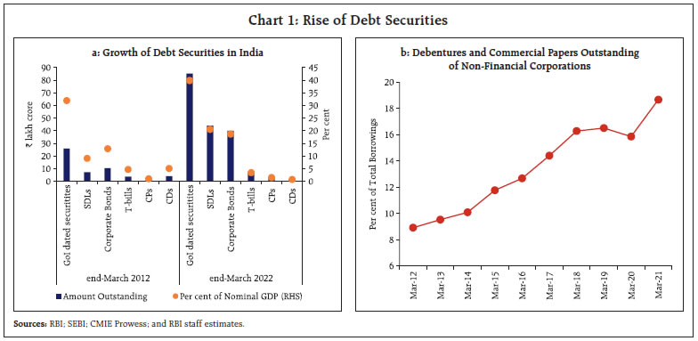 Scale and Scope of Debt Mutual Funds The assets under management (AUM) of debt MFs stood at ₹12.6 lakh crore at end-September 2022, increasing from ₹3.7 lakh crore at end-March 2012, registering a compounded annual growth rate of 12.2 per cent (Chart 3). However, the share of assets managed by debt mutual funds in the overall mutual fund industry decreased to 32.8 per cent from 63.8 per cent during this period with rise in other categories of mutual funds, viz., equity, balanced, and other schemes. 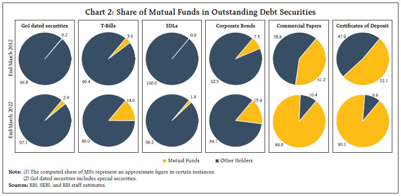 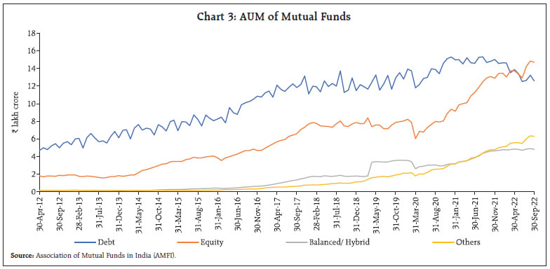 Open-ended debt schemes1, i.e., schemes available for subscription and repurchase by investors on a continuous basis, account for 98.5 per cent of the AUM held with debt MFs at end-September 2022. Among the open-ended debt schemes category, liquid funds, i.e., funds with investment in debt/money market securities with maturity of up to 91 days account for maximum share of 28.4 per cent (Chart 4 and Annex 1). 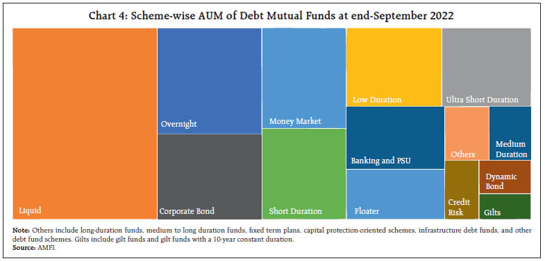 At end-June 2022, corporates remained the largest class of investors, contributing ₹8.5 lakh crore to the AUM of ₹12.5 lakh crore of debt MFs, typically investing in funds of shorter duration. High Net-worth Individuals (HNIs) are the second largest class of investors, accounting for ₹3.2 lakh crore of AUM and favouring funds of relatively longer duration since their investment objectives are likely to be different from those of corporates (Chart 5). 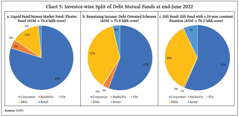 In contrast to Indian scenario, retail investors hold vast majority of MF assets (nearly 88 per cent), including substantial money market fund assets, in the US (Chart 6). Institutional investors hold a relatively small share of MF assets (nearly 12 per cent), mostly in money market funds2. International experience suggests that countries with more-developed capital markets tend to have more-developed fund industries3. However, households prefer banking products over regulated funds in countries where banks have historically played a significant role in the financial ecosystem (e.g., Japan). In 2021, the annual Investment Company Institute (ICI) survey of mutual fund ownership found that 59.0 million, or 45.4 per cent, of households in the United States owned MFs4. While equity assets form major share of MF assets, developed economies like US are witnessing increased flows to debt MFs due to ageing population. 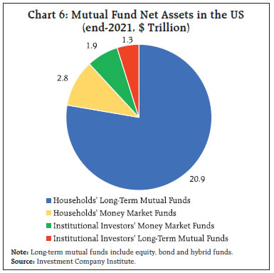 Debt Portfolio of Mutual Funds The aggregate debt portfolio of MFs in India (including debt, balanced funds, etc.) has witnessed structural transformation over the years; CDs used to account for the maximum share of the debt portfolio but have since lost their share to other debt instruments. Presently, MFs maintain most of their debt portfolio in corporate bonds, playing an active role in meeting the financing requirements of the corporates (Chart 7). CPs also account for a sizeable share of MFs’ portfolio. However, in the recent period, the combined allocation to corporate bonds and CPs has moderated to 42.2 per cent at end-July 2022 from a peak of 77 per cent at end-July 2018, amid risk aversion following the Infrastructure Leasing & Financial Services Limited (IL&FS) episode5 and COVID-19 pandemic. Further, credit risk funds, i.e., funds with a minimum of 65 per cent of total assets in AA and below rated corporate bonds, have not generated much interest amongst investors and have been witnessing a consistent decline in AUM since April 2019. Meanwhile, MFs have increased their investments significantly in Government securities, T-bills, and TREPS6. The proportion of Government securities (including T-bills) in the debt portfolio of mutual funds has increased in the recent period, reaching 27.2 per cent at end-July 2022. The rise in investment in TREPS to some extent, may be explained by the growing popularity of overnight funds, i.e., funds that invest in overnight securities having a maturity of one day - as indicated by the co-movement in MFs’ investments in TREPS and AUM of overnight funds (Chart 8). The AUM of overnight funds has grown by almost ten times between April 2019 and July 2022 amid a notable shift in preference from liquid funds to overnight funds. This shift is primarily a result of the SEBI’s introduction of a graded exit load7 on investors who exit the liquid fund within seven days of their investment8. Further, SEBI’s initiative to allow MFs to offer instant access facility9 in overnight schemes has increased the attractiveness of overnight funds10. 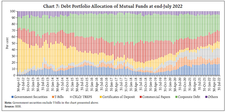 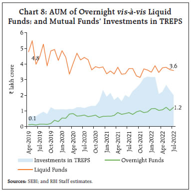 III. Determinants of Debt Fund Flows: Some Discussion The cash flows generated by non-financial corporates has tracked the net change in AUM of corporates in debt MFs quite well in the recent period (Chart 9). Strong operational performance translates into higher cash flows and may be expected to translate into higher savings and investments by corporates in financial instruments, including the mutual funds. Fund flows to short-term debt mutual fund schemes exhibit a high positive correlation amongst themselves, except in the case of overnight funds (Chart 10.a). There exists a high negative correlation between monthly net flows to debt mutual funds and corporation tax payments (r = -0.67). Further, there has been some seasonal pattern in flows into debt MFs. During quarter ending month, with an increase in corporates’ tax payments, flows into debt mutual funds exhibit a decline or turn negative due to redemption by corporates (Chart 10b). 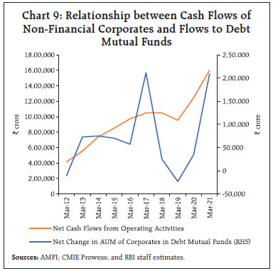 The impact of Covid-19 on debt MFs was exacerbated in March 2020 as it coincided with the tax filing month. The heightened volatility during Covid-19 led to redemption pressures and liquidity strains, accentuated by shallow corporate bond markets. It also led to the closure of some debt MF schemes, which sent chills across the domestic financial markets and created fears of similar winding-up by other debt MFs. Subsequently, to ease the liquidity pressures and safeguard financial stability, the Reserve Bank of India had stepped in with a Special Liquidity Facility for MFs (SLF-MF) amounting to ₹50,000 crore, which helped in restoring confidence in the financial markets. In the recent period of H2: 2021-22 and H1: 2022-23, debt MFs witnessed net redemptions as investors stayed away to avoid price risk amid hardening of bond yields. 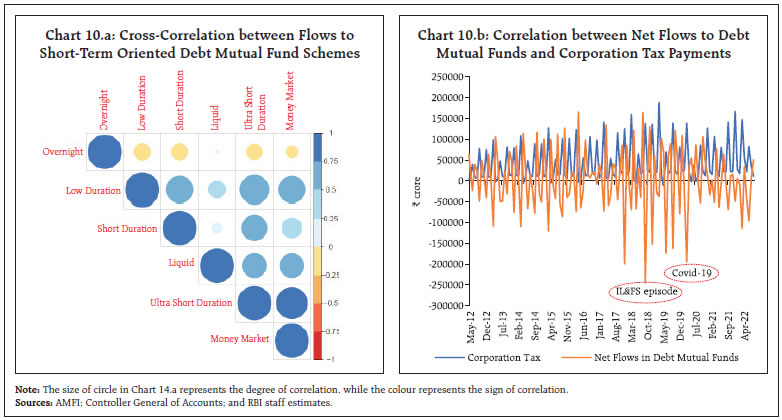 IV. Relationship between Net Flows and Returns on Debt Mutual Funds In recent years, debt mutual funds have gained increasing prominence in the process of financial intermediation. Accordingly, the possibility of any spillover risks in the financial system emanating from such non-banking intermediaries has increased. Therefore, it is important to understand the behavioural pattern of investors in debt mutual funds, and linkages between flows and returns (Chart 11). The objective is to understand whether a sharp drop in bond prices (or lower returns on debt MFs) can trigger a cascade of redemptions by mutual fund investors and/or whether any episode of sharp redemptions can exert significant downward pressure on bond prices (and reduce the net assets value of debt MFs). 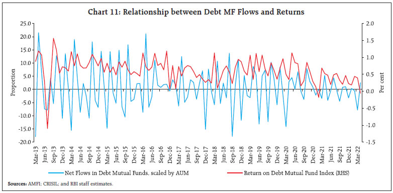 As the debt mutual fund industry and non-bank financial intermediation grow rapidly, understanding the relationship between fund flows and returns becomes important. Although an enormous amount of literature is available for equity mutual funds, literature on determinants of flows to debt mutual funds is limited in the Indian context. Fortune (1998) suggests that in the US (1985-1996), net new money flows into debt-type funds are predictors of returns on debt securities while equity fund flows do not predict returns on either equities or bonds. The study further finds that security returns have a contemporaneous and direct effect on fund flows. Another study in the context of US uses data from 1992-2005 period and finds that bond fund investors chase funds that are the performance leaders on a risk-adjusted basis rather than on the basis of raw returns (Zhao, 2005). The author also finds poor long-term equity market returns tends to increase investors’ investments in government security funds and finds that most bond fund investors are sensitive to expenses; they avoid funds with high operating expenses. In the Indian context, a study identifies the presence of seasonality factors in both debt and equity fund flows (Madhumathi et al, 2012). It finds that market volume and volatility influence debt mutual fund flows during the period July 2005 to August 2012. In the wake of this, an empirical exercise has been undertaken to understand the relationship between net flows and returns on debt mutual funds, i.e., whether flows impact returns and/or returns impact flows in India. Further, in the second part of the section, we explore these dynamics in the presence of various market fundamentals, which are used as exogenous variables. As per the best of our knowledge, no study has been done on the similar subject so far in India. Data and Methodology The monthly data on net flows are obtained from Association of Mutual Funds in India (AMFI) for the period March 2013 to March 2022. Net flows are normalised by the previous month’s net AUM to control for the increasing trend in flows (Remolona et. al, 1997). Further, the net normalised flows have been de-seasonalised to control for seasonal variations. To arrive at a proxy for returns on debt mutual funds, we construct a weighted average index using monthly data on CRISIL benchmark indices against which the performance of similar type of debt mutual fund schemes are tracked. While doing so, the implicit assumption is that the actual return on debt mutual funds shall track the return on their respective CRISIL benchmark indices. For this exercise, we use 15 different CRISIL benchmark indices, viz., CRISIL overnight index, liquid fund index, ultra-short-term debt index, low duration index, money market index, short term bond fund index, medium-term debt index, medium to long term debt index, long term debt index, composite bond index, corporate bond composite index, short term credit risk index, banking and PSU debt index, dynamic gilt index and 10-year gilt index.11 These indices, which are used as benchmarks for 15 types of open-ended debt mutual funds12, are aggregated using average assets under management held under such mutual funds during April 2019-March 202213, as weights. CRISIL liquid fund index accounts for the highest weight of around 33 per cent in the aggregate index. Summary statistics show that the volatility of monthly flows is high as compared to returns. The correlation coefficient is positive and statistically significant suggesting that flows and returns move together. The stationarity results are shown in Table 1. Both the series are stationary. To assess the inter-temporal relation between flows and returns, a reduced form bivariate VAR model is deployed14 as shown below: 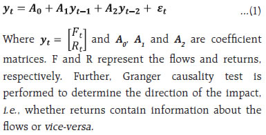 The results of the reduced-form bivariate VAR model are presented in Table 2. Lag length selection was done based on the Bayesian Information Criteria (BIC), which shows lag selection at 2. Flows are significantly influenced by one month lagged returns [Table 2(1)]. Flows exhibit strong autocorrelation up to two months lag. The R2 for flows equation is 0.31 implying past returns do indeed contribute to current flows. However, returns are not impacted by previous months’ flows [Table 2 (2)] but are impacted by one month lagged returns. Also, the R2 for returns equation is low implying that capacity of flows to explain the returns is marginal. The results of the Granger Causality test between flows and returns are reported in Table 3. The null hypothesis that “returns do not Granger-cause flows” is rejected at a very high level of statistical significance, suggesting that past values of returns contain significant information about current flows. However, we fail to reject the null hypothesis “flows do not Granger-cause returns,” implying that the past value of flows does not contain any information about current returns. Thus, one-way Granger causality is established between flows and returns, i.e., past values of returns influence current flows but not vice-versa. For diagnostic checks, we apply the Portmanteau test to check for serial correlation in the residuals of the VAR-(2) model and ARCH test to check for heteroscedasticity in the residuals of the VAR-(2) model. No heteroscedasticity and serial correlation were found in the residuals of the VAR-(2) model. To test for structural break in the residuals, we apply the cumulative sum (CUSUM) test. No structural beak in the residuals was noted (Annex 2). The impulse response functions are presented in Annex 3, which corroborate the findings. As an improvement to the reduced-form bivariate VAR and the causality test, we analyse the relationship between flows and returns on debt mutual funds in the presence of market fundamentals. For doing this, we incorporate the following variables viz., corporate bond spreads to measure credit/default risk, Index of Industrial Production as a proxy for the state of the economy, banks’ average savings and term deposits rate to measure rate of return on competitive savings instrument, average amount outstanding under RBI’s liquidity adjustment facility to measure liquidity conditions, and CPI inflation rate15 (Table 4). To understand the state of the economy variable, we use the concept of growth cycles. The growth cycle is defined as the alternate sequence of high and low growth phases (rather than expansion and contraction in the levels of general economic activity) through deviations of the actual growth rate of the economy from the long-run trend growth rate. Contraction in the growth cycle indicates a slowdown in economic activity while an expansion indicates a surge in the economic activity. Thus, a dummy variable representing 0 (contraction) and 1 (expansion) are used. To obtain this, we first extract the cyclical component of the IIP (log) series. One of the most widely used detrending methodologies is the Hodrick- Prescott (HP) filter (Hodrick & Prescott, 1980). However, according to King and Rebelo (1993), HP filter seriously alters measures of persistence, variability, and co-movement. As a result, we use band-pass filters proposed by Baxter and King (1999) and Christiano and Fitzgerald (2003). Band pass filters retains components of the time series with periodic fluctuations between 6 quarters (18 months) and 32 quarters (96 months), while suppressing components at higher (irregular) and lower frequencies (trend). These filters approach the trend-cycle decomposition and smoothing problem in the frequency domain. In our work, we use the asymmetric Christiano-Fitzgerald filter (CF) to isolate the trend and cyclical component. The CF filter puts different weights to each observation and hence the filter is asymmetric. The cyclical component is standardised before the application of the dating algorithm. We use the Harding-Pagan algorithm (2002) to identify expansion and recession. The selection of various macroeconomic variables has been done on the basis of existing literature [such as Kopsch et. al (2015)], and common understanding. In the presence of market fundamentals, if we obtain unidirectional causality from returns to flows as obtained earlier, then this would indeed show that it is the returns which drive the debt mutual fund flows. The debt mutual fund flows are simply responding to changes in returns. The following regression equations incorporating market fundamentals are used: 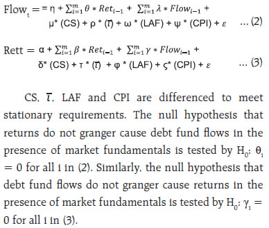 The results reporting the direction of the flows-returns relationship in the presence of market fundamentals are presented in Table 5. The results obtained are similar to earlier results. The results reject the hypothesis that past returns do not granger cause current flows. It shows that in the presence of market fundamentals, flows exhibit auto-correlation up to two lags. Further, flows are impacted by one-month lagged returns and credit spreads. The primary objective behind saving/ investing in debt mutual funds is safety of principal and any increase in credit risk seems to be acting as deterrence of flows to debt mutual funds. Table 5(2) shows that we fail to reject the null hypothesis of past flows granger causing current returns. Returns are affected by one month lagged returns and CPI. An increase in inflation drives up the expectation of monetary policy tightening by the central bank, which may be leading to increase in bond yields and fall in bond prices (due to an inverse relationship between yields and prices). A fall in bond prices translates into a declining return on mutual fund holdings. The R2 and adjusted R2 have increased marginally for flows and returns as compared to Table 2 suggesting that exogenous variables do not contribute much in explaining variation in current flows and current returns. The flows into the debt MFs exhibit seasonality, witnessing redemption by corporates at every quarter-end, especially at the end of the financial year, mainly to meet tax payment obligations. The empirical exercise suggests that past returns contain information about current flows in debt MFs but not vice-versa. A period of dwindling returns can lead to outflows from debt MFs. This is true even in the presence of various market fundamentals. Some of these fundamental market indicators also play a role in determining flows and returns. Credit spreads are found to be inversely related to flows, and CPI inflation is found to be inversely associated with returns. References Baxter, M., & King, R. G. (1999). Measuring business cycles: approximate band-pass filters for economic time series, The Review of Economics and Statistics, 81(4), 575-593. Christiano, L. J., & Fitzgerald, T. J. (2003). The band pass filter, International Economic Review, 44(2), 435-465. Fortune, P. (1998). Mutual funds, Part II: Fund flows and security returns. New England Economic Review, 3-22. Harding, D., & Pagan, A. (2002). Dissecting the cycle: a methodological investigation. Journal of monetary economics, 49(2), 365-381. Hodrick, R. J., & Prescott, E. C. (1980). Postwar US Business Cycles: An Empirical Investigation [Discussion paper No. 451]. Centre for Mathematical Studies in Economics and Management Science, Northwestern University, Evanston, 111. King, R. G., & Rebelo, S. T. (1993). Low frequency filtering and real business cycles. Journal of Economic dynamics and Control, 17(1-2), 207-231. Kopsch, F., Song, H. S., & Wilhelmsson, M. (2015). Determinants of mutual fund flows. Managerial Finance. Madhumathi, R., Gopal, N., & Ranganatham, M. (2012, December). Determinants of Debt and Equity Mutual Fund Flows in India. In XI Capital Markets Conference (pp. 21-22). Remolona, E. M., Kleiman, P., & Gruenstein Bocain, D. (1997). Market returns and mutual fund flows. Economic Policy Review, 3(2). Zhao, X. (2005). Determinants of flows into retail bond funds. Financial Analysts Journal, 61(4), 47-59. Classification of Debt Schemes
  ^ The authors are from the Department of Economic and Policy Research. * The authors express their gratitude to Shri Sanjay Hansda for his encouragement and valuable guidance. The authors also thank Kaustav Sarkar, Chaitali Bhowmick, Amit Pawar and internal referee for their insightful comments. Data support from CRISIL is also duly acknowledged. The views expressed in this article are those of the authors and do not represent the views of the Reserve Bank of India. 1 These schemes do not have a fixed maturity period. Investors can conveniently buy and sell units at Net Asset Value (NAV) which is declared daily. The key feature of open-end schemes is liquidity. 2 https://www.icifactbook.org/pdf/2022_factbook.pdf 3 https://www.ici.org/system/files/2021-05/2021_factbook.pdf 4 https://www.ici.org/system/files/2021-10/per27-12.pdf 5 During 2018, IL&FS, a systemically important non-deposit accepting core investment company (CIC-ND-SI) defaulted on repayments of CPs, nonconvertible debentures (NCDs) and bank loans which resulted in subsequent rating downgrades of IL&FS and a few other NBFCs. 6 Erstwhile Collateralised Borrowing and Lending Obligation (CBLO). 7 Graded exit load means applicability of exit load based on time interval between date of subscription and date of redemption, i.e., higher exit load applies if an investor exits MF within one day of subscription in comparison to an investor who exits on the sixth day of subscription. 8 SEBI’s circular on ‘Risk management framework for liquid and overnight funds and norms governing investment in short term deposits’ dated September 20, 2019. 9 Instant access facility is an option available to investors to get access to their funds within a short window of giving the redemption request. 10 SEBI’s circular on ‘Deployment of unclaimed redemption and dividend amounts and instant access facility in overnight funds’ dated July 30, 2021. 11 These indices seek to capture coupon and price returns of the underlying portfolio comprising of money market and debt securities. 12 These account for around 90 per cent of total AUM held under debt mutual funds. 13 The AMFI’s data on new categories of mutual fund schemes are available from April 2019 onwards only while CRISIL’s benchmark indices data for such schemes are available for prior period also. 14 To understand the dynamic relationship between variables as well as their interaction with one another, VAR is a natural choice. 15 In another model, we had additionally used VIX as one of the exogenous variable, however our results broadly remained similar to the earlier results. | ||||||||||||||||||||||||||||||||||||||||||||||||||||||||||||||||||||||||||||||

Share this page:


Install the RBI mobile application and get quick access to the latest news!
Scan the QR code to install our app


Page Last Updated on:


