 IST,
IST,
RBI WPS (DEPR): 09/2013: Corporate Pricing Power, Inflation and IIP Growth: An Empirical Investigation
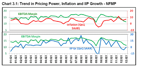
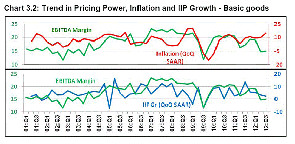
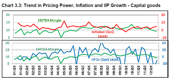
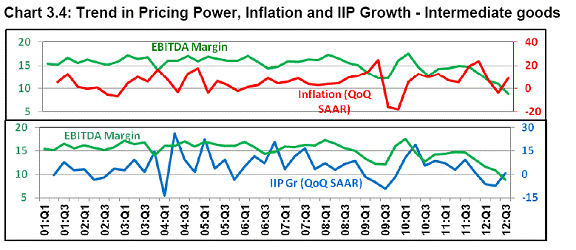
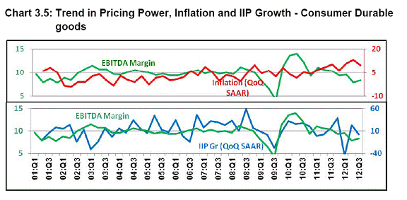
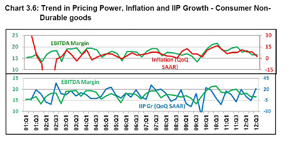
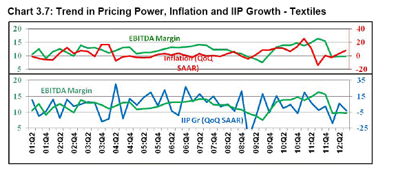
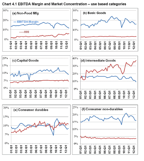
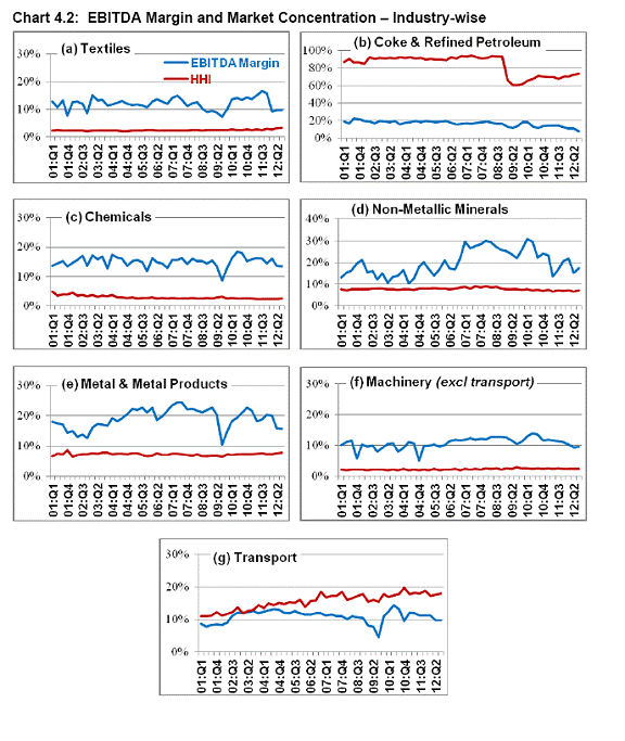
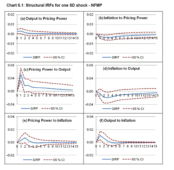
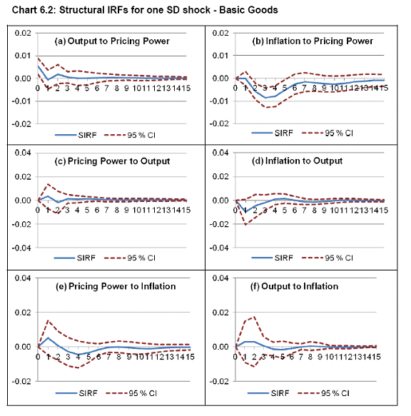
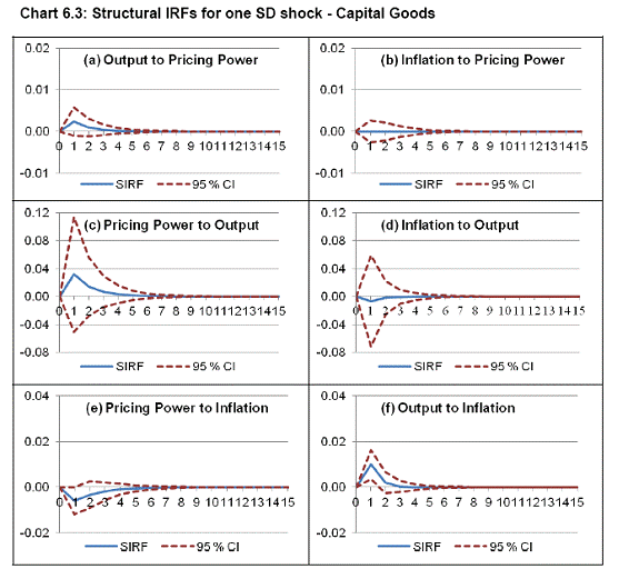
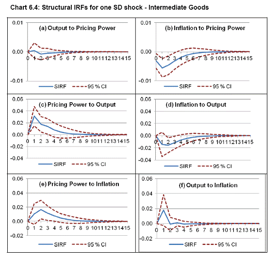
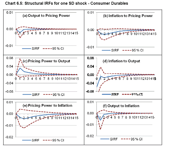
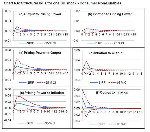
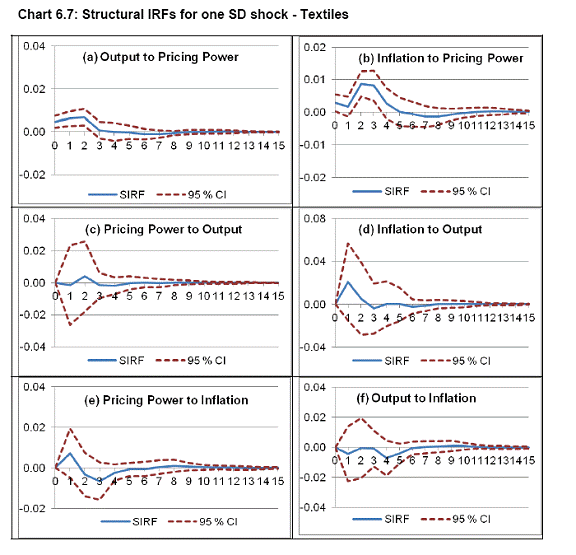
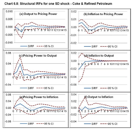
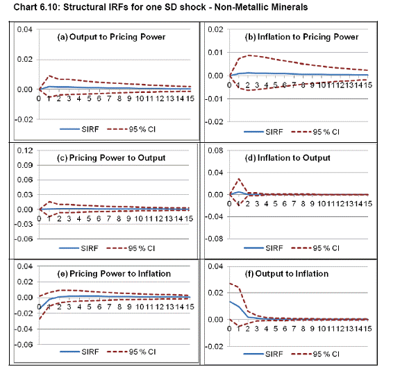
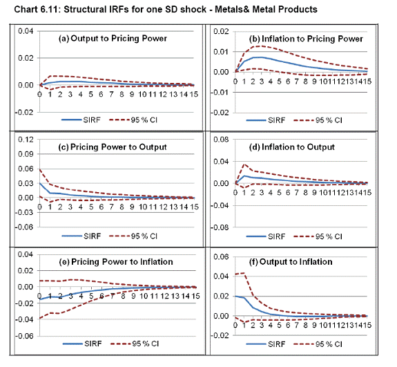
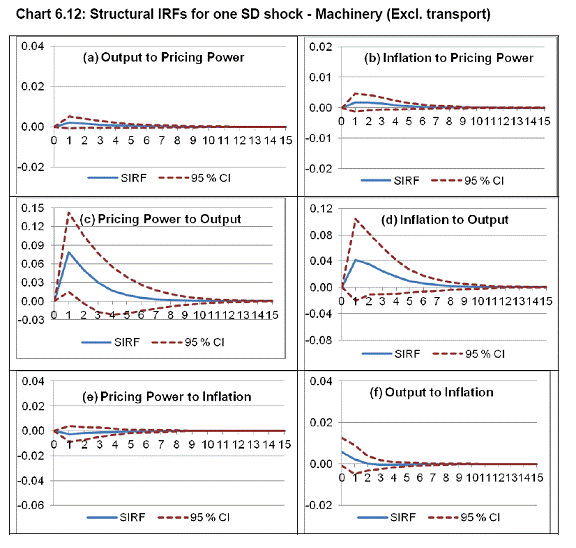
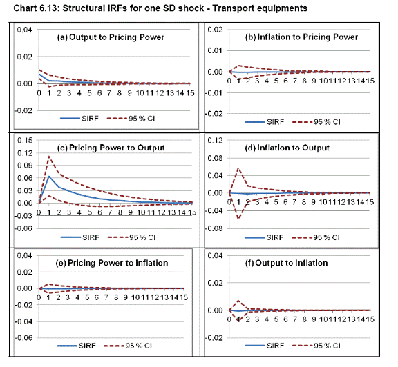
| Press Release RBI Working Paper Series No. 09 Abstract 1Pricing power measures the extent to which a business can pass on the increases in input costs to consumers through increases in the prices of finished goods. The corporate pricing power in India has declined since 2009-10:Q1. Production has also fallen sharply since 2010-11:Q3. However, WPI inflation has been sticky and remained at a relatively higher level. In this context, this paper attempts to examine the relationship among corporate pricing power, inflation and growth in India under a structural VAR framework keeping in view the role of market structure and cycles of the economy. Empirical results indicate that pricing power has a statistically significant and positive impact on output growth in case of non-food manufacturing products. The impact of pricing power on inflation is also positive but relatively subdued. A fall in pricing power, therefore, is followed by higher and faster decline in output than in inflation. JEL Classification: L11, E31, C32 Keywords: Pricing Power, Inflation, Growth, Market Structure 1. Introduction In an inflationary environment, pricing power plays an important role in predicting corporate performance. It measures the extent to which a business can pass on the increases in input costs to consumers through increases in the prices of finished goods. If the firms are able to pass through the increase in input costs to their customers and protect their profit margin, they are supposed to have pricing power. In a monopolistic market structure, businesses with a high value added are likely to be able to pass on all inflationary costs. The changes in market power influence the degree to which prices adjust to productivity and inflation shocks. This is more so when the sellers’ ability to change prices is constrained. On the other hand, lower and more stable inflation is considered a key factor behind the reduction in the degree to which firms pass through both price increases at competing firms and cost increases due to exchange rate movements or other factors (Taylor, 2000). In standard economic theory, higher use of labour, capital and other inputs pushes production costs up in an expansionary phase of economy which subsequently gets reflected in higher product prices. But when the economy operates below its potential, the increase in production cost slows down, which restricts firms’ ability to raise prices. This suggests that pricing power of firms depends on inflation, market power as well as the level of economic activity. Empirical evidence, however, has been varied concerning the exact nature of this relationship. In the Indian context, there is empirical evidence showing that there has been a reduction in pricing power during 2009-20122. Decline in pricing power was broad based and was not of similar magnitude across industries. During the same period, monetary policy remained contractionary. However, the wholesale price index (WPI) inflation for the non-food manufacturing products (NFMP) has not reacted by similar downward shift and has been rather sticky till the recent period. Explaining this counter intuitive anomaly is the basic purpose of this paper. The context of the issue is as follows. In the aftermath of the 2008 global financial crisis, India’s GDP growth declined significantly from 9.3 per cent in 2007-08 to 6.7 per cent in 2008-09 partly due to the impact of external demand shocks on domestic economy. Through expansionary monetary and fiscal policy actions, growth recovered quickly during 2009-10 and 2010-11 to 8.6 per cent and 9.3 per cent, respectively. Subsequently, however, due to domestic and external factors, GDP growth slowed down to 6.5 per cent in 2011-12. This decline was broad based and was more pronounced for industrial sector. During the same period, inflation rate in India rose from 4.7 per cent in 2007-08 to 8.1 per cent in 2008-09 and fell to 3.8 per cent in 2009-10. Thereafter, the inflation rate backed up and stayed near double digits during 2010-11 and 2011-12. Besides an elevated headline inflation, a kind of generalised price pressure kept non-food manufactured products inflation at a higher level. Akin to GDP growth trajectory, performance of Indian corporates was also diverse. Their pricing power, as can be measured by the operating profit margin viz. ‘Earnings Before Interest, Taxes, Depreciation, and Amortisation’ (EBITDA) to sales ratio, declined sharply from its highest level at 17.5 per cent in 2009-10:Q1 to 11.5 per cent in 2011-12:Q33. The above discussion brings out the fact that corporate pricing power in India has declined since 2009-10:Q1. While production has fallen sharply since 2010-11:Q3, WPI inflation has been sticky and remained at a relatively higher level. Reserve Bank, on its part, hiked the policy interest rate by a cumulative 375 basis points between March 2010 and October 2011. Given these facts, the paper analyses the questions viz., why lower pricing power did not get translated into lowering in price rise? Is it broad-based across industry? Do market power and business cycles have any role in explaining such behaviour? In this paper, we have tried to address some of these issues. Towards this, we explicitly acknowledge that the degree of pass-through or pricing power of corporates should not be taken as exogenous to the inflationary environment. Following Boivin et al. (2009), we argue that sticky prices and economic activity do fluctuate in response to sector-specific shocks, even though, they tend to respond only sluggishly to aggregate macroeconomic shocks such as monetary policy shocks. These suppositions underscore the need for sector specific analysis. Accordingly, this paper examines the relationship between corporate pricing power, inflation and growth in India for the aggregate as well as the standard use-based industry classifications and broad industry groups. In order to capture the dynamic endogenous relationships among the variables, a structural vector auto regression (SVAR) framework is used, after controlling the effects of market power and business cycles. Overall results indicate that macroeconomic consequences of persistently sticky inflation and decline in industrial demand are pushing pricing power downwards and on the other hand, the fall in pricing power is more consequential in further fall in the output. The paper is organised as follows. In Section 2, we review the literature on the impact of pass-through or pricing power of corporate on growth and inflation covering briefly both theory and empirical evidence, particularly for advanced economies. Section 3 briefly captures some stylised facts based on the trends in corporate pricing power, inflation and growth in India. In order to capture the diverse response of pricing power across industries, information is presented across various use-based classifications and industry groups. The role of market power and business cycles in determining pricing power is presented in Section 4. Subsequently, in Section 5, we present the empirical model using a SVAR framework. Empirical results are discussed in Section 6. Finally, Section 7 presents the conclusions, with some policy discussions. 2. A brief review of literature Economists have long studied the relationship between resource utilisation and inflation. It is rightly acknowledged that the changes in the pricing power of firms affect the relationship between output and inflation. Generally, the relation between inflationary environment and pricing behaviour is studied under two strands of economic theories - monetary theory and the theory of price setting with imperfect competition. Theories of price adjustment have dealt with imperfect competition models where firms have some market power (Blanchard and Kiyotaki, 1987). The staggered price setting models, as proposed by Ball and Cecchetti (1988) indicated that observed changes in pricing power could be either due to inflation persistence expectation or input cost fluctuations. That is, the extent to which a firm adjusts to rising input costs is guided by the expected persistence of that increase. If the persistence of inflation is low, firm’s expected persistence of cost and price changes get reduced which finally results into declining pricing power. So the role of monetary policy in delivering a low and stable inflation becomes important for firms pricing behaviour. This was mostly the case for the United States during the late 1990s. Before the onset of 2008 global financial crisis, one of the most remarkable changes in the global economy pertaining to monetary policy was the sharp reduction in exchange rate pass-through (Taylor, 2006). This pass-through was fairly broad based, both at traded commodity level as well as aggregate price indices (Devereux and Yetman, 2003). Some, including Rogoff (2006), attributed this decline to globalisation and the reduced pricing power of firms due to foreign competition. But Taylor (2006) credited this decline in pricing power to monetary policy changes. He emphasised that with the adoption of inflation targeting, implicitly or explicitly, persistence of exchange rate variability affecting prices declined. Thus, firms preferred postponing of pass-through of increased input cost on account of adverse effect of exchange rate, as its effect turned temporary. Nominal prices in the economy fluctuate for many reasons. Empirical studies clearly suggest three different outcomes of the responsiveness of nominal prices to various shocks - it is incomplete, it fluctuates over time and it has positive correlation with average inflation. For example, for the U.S. and other developed countries, as the rate of inflation over time remained subdued, firms’ response to nominal price setting to changes in costs actually declined (Taylor, 2000). However, researchers like Choudhri and Hakura (2006), Campa and Goldberg (2005), Devereux and Yetman (2002) presented contrary evidence and argued that the pass-through of nominal exchange rate movements to consumer prices was indeed increasing. They interpreted the exchange rate movements as exogenous cost shocks. Similar evidence was also observed by Gagnon (2007) for Mexico. In addition, empirical evidence also showed a negative relation between the average mark-up and inflation trend (Gali and Gertler, 1999; Banerjee, Mizen, and Russell, 2007). Majority of empirical evidence of sticky-price models was primarily developed to explain the aggregated price behaviour of firms. However, Boivin et al. (2009) argued that ‘these models appeared to explain poorly the behaviour of more disaggregated price series and models with relatively flexible sectoral prices did not seem to explain the empirical evidence obtained from aggregate series’. They found differential impact on sectoral prices to sector-specific shocks. In particular, monetary policy shocks had significantly lagged impact on a large number of price series. Earlier on the similar lines, Bils and Klenow (2004) for the U.S, Fabiani et al. (2004) for Italy and Alvarez et al. (2006) for Spain and the Euro area used disaggregated price data and broadly observed that higher inflation led to more frequent price changes. Although there exists a large literature on price setting behaviour, most of the research in this area has primarily been conducted in developed countries. On the contrary, little research has taken place within the context of developing countries on price setting behaviour. Particularly in the Indian context, evidence of the impact of monetary policy on corporate pricing behaviour has been limited. Indirectly some authors provided weakening of corporate sector performance during 1990-2002 in terms of profitability and which was contributed partly by adverse interest rate/foreign exchange movements (Topalova, 2004). Recent decline in pricing power of Indian companies and its possible impact on inflation has been well documented in the Reserve Bank’s quarterly macroeconomic analysis (RBI, 2012). With slowdown of the economy, waning of the pricing power was mostly attributed to moderation in demand as also lower non-oil commodity prices. However, its impact on inflation, particularly on non-food manufacturing products, was slow and prolonged over a period of time. In the next section, we discuss how pricing power of Indian companies has evolved over time and its dynamic relation with growth and inflation. 3. Trends in corporate pricing power, inflation and growth: some stylised facts Manufacturing sector holds an important position in India’s economic growth due to its strong linkages with other sectors of the economy and its potential to create employment. Further, activity of the manufacturing sector determines the overall business cycle. As regards inflation, the manufacturing sector probably gets more affected than the services sector mainly due to the dependence of the former on raw materials. In a high inflation scenario, the bottomline is adversely affected due to increase in cost of the raw materials. As a result, the selling price of the product might also rise. Thus, the higher selling price compensates the increase in cost price and the profit margin remains protected or gets fatter. However, the realisation in terms of higher selling price heavily depends on the demand situation. With increased price resulting to declining demand, the pass-through of the increased cost becomes difficult. Therefore, the pricing power of the corporates starts falling. On the other hand, in a low inflation scenario the cost of input as well as the selling price - both remain lower, limiting the prospect of a better profit margin. In our study, the relationship between corporate pricing power, inflation and industrial production is examined focusing on the non-food manufacturing sector based on quarterly data for the period 2000-01:Q1 to 2011-12:Q3. Non-food manufacturing products (NFMP) in this paper include the ‘Manufacturing’ sector of National Industrial Classification (NIC) - 2004 excluding the manufacturing of food products and beverages. The weights of these different categories in Wholesale Price Index (WPI) and in Index of Industrial Production (IIP), however, are not similar (Appendix Table 3.1). The movements in inflation and IIP growth may be subject to this limitation. Profit margin for non-food manufacturing products has been on gradual upward movement since 2000-01 and reached peak at 17.4 per cent in 2006-07:Q3. After a marginal fall next quarter, it again went up in 2007-08:Q1. Thereafter, it started gradual decline and accentuated further during the financial crisis of 2008-09 touching the bottom in nine years at 11.1 per cent in 2008-09:Q3. It rebounded strongly in the next two quarters to reach the peak again in 2009-10:Q1. However, the performance could not be sustained and there has been almost secular decline since then. Inflation moved in a cyclical fashion in the range of zero to 10 per cent, except in few quarters. It was negative during 2008-09:Q3 to 2009-10:Q1 and was above 10 per cent in 2010-11:Q4. The growth in IIP has been quite volatile during the entire period. In recent periods, it has fallen sharply since 2010-11:Q3. However, inflation appeared to be sticky and not following the trend in corporate profit margin and IIP growth (Appendix Chart 3.1). Dynamics of these variables at use based classification and select industry group levels are explored in detail in the subsequent sections. 3.1 Descriptive analysis of pricing power, inflation and growth: Use based classification For analysing the common trends, NFMP can be further disaggregated based on five use based categories, viz., (i) Basic Goods (minerals, coal, diesel, electricity, iron and steel etc.), (ii) Capital Goods (machineries, plant and machine equipment, computers, bus, truck, etc.), (iii) Intermediate Goods (non-food articles, naphtha, lubricants, oil cakes, textiles etc.), (iv) Consumer Durables (gold, silver, wood products, air conditioner, refrigerator, TV, motor vehicles etc.) and (v) Consumer Non-Durables (food, beverages, petrol, kerosene, clothing, paper, footwear, medicines etc.). In case of basic goods, inflation and IIP growth moved more or less in tandem during the period (2000-01:Q1 to 2011-12:Q3). The EBITDA margin peaked at 23.3 per cent in 2006-07:Q1 and remained at a high level for more than two years before falling during the crisis year 2008-09. Inflation was at its highest levels during 2007-08:Q4 and 2008-09:Q1. Post financial crisis, inflation has been sticky at around 10 per cent except in 2010-11:Q2. Though there was some recovery in 2010-11:Q4 and 2011-12:Q1, EBITDA margin, on the other hand, displayed a declining trend after 2010-11:Q1 (Appendix Chart 3.2). Major constituents of basic goods (viz. basic metals, ATF, diesel) being imported, inflation might have been sticky and was not affected much by the fall in EBITDA margin. EBITDA margin in capital goods remained close to 10 per cent or less till 2005-06:Q1 and then above 10 per cent till 2011-12:Q1. It was less volatile and much lesser affected during the financial crisis as compared with the other categories. Since its peak at 13.7 per cent in 2009-10:Q3, the EBITDA margin has started falling marginally in a gradual manner. It is important to note that inflation was comparatively lower in this category. It moved in a range between zero and 5 per cent since 2009-10:Q2. The IIP growth has been much more volatile and was on declining trend since 2010-11:Q2 (Appendix Chart 3.3). In intermediate goods, the EBITDA margin was mostly above 15 per cent during 2000-01 to 2007-08 barring few quarters. From the high at 17.3 per cent in 2007-08:Q1, it declined sharply to a low of 12.2 per cent in the middle of 2008-09. Then it bounced back in the next two quarters to the peak of 17.5 per cent in 2009-10:Q1. However, it fell again sharply in the next two quarters and reached 12.8 per cent in 2009-10:Q3. Since 2010-11:Q3, the EBITDA margin was on steep unidirectional fall and it fell to below the financial crisis level since 2011-12:Q1. The fall in IIP growth has also been sharp since 2010-11:Q4 except a rebound in 2011-12:Q3. Inflation in intermediate goods, more often than not, followed the EBITDA margin. It also came down sharply from a high level of 23.8 per cent in 2010-11:Q4 in next two quarters (Appendix Chart 3.4). The intermediate goods mainly comprise of manufactured non-food articles (though oil cake is an important input for milk). The inflation in this category is probably more closely related to manufacturing activities. Major constituents of consumer durables goods are gold and silver. The EBITDA margin fell sharply in 2008-09:Q3 but rebounded strongly in the next three quarters before reaching the peak at 14.0 per cent in 2009-10:Q2. Thereafter, it moved in a steep declining trend. Inflation was seen to be low and below 5.0 per cent for a long period 2000-01:Q4 to 2008-09:Q1 except on a few occasions. It did not fall too much during the financial crisis also. Contrary to the steep fall in EBITDA margin, inflation was in an up-trend since the lows of 2009-10:Q2. The IIP growth was quite volatile during this period (Appendix Chart 3.5). For consumer non-durables goods, EBITDA margin was seen relatively high and was not much affected by the financial crisis (the lowest was at 13.4 per cent in 2008-09:Q3). Inflation and EBITDA margin moved more or less in similar direction. Major constituent under consumer non-durables goods category are food items, and which recorded high inflation during 2009-10. Since 2009-10:Q3, both inflation and EBITDA margin displayed a declining trend (Appendix Chart 3.6). To summarise, basic goods, intermediate goods and consumer non-durables recorded higher level of profit margin than capital goods and consumer durables. Also, profit margin in these three categories appeared less rigid. However, profit margin in all the categories declined since 2009-10:Q3. Importantly, the profit margin in intermediate goods fell below the lows during the financial crisis year and at lowest level in the last 12 years. Like profit margin, inflation in capital goods and consumer durables was less volatile and moved in narrower range as compared with other categories. Growth in IIP was quite volatile in case of capital goods, consumer durables and non-durables and relatively less volatile for basic and intermediate goods. 3.2 Descriptive analysis of pricing power, inflation and growth: Industry sectors Apart from use based categories, some select broad industry groups, identified using NIC 2-digit industry level classification, were also considered. The industries selected for the analysis were (i) ‘Textiles’, (ii) ‘Coke & Refined Petroleum’, (iii) ‘Chemicals’, (iv) ‘Non-Metallic Minerals’, (v) ‘Metal and metal products’, (vi) ‘Machinery (excluding transport)’ and (vii) ‘Transport equipments’. As observed at industry level, the trend in EBITDA margin, inflation and IIP growth was not uniform. In ‘Textiles’, ‘Chemicals’ and ‘Metal & Metal Products’ industries, all the three variables displayed decline towards the end of 2010-11 and then in 2011-12. The EBITDA margin in the ‘Textiles’ industry rose to its peak in the last twelve years in the aftermath of 2008-09 crisis. But it fell sharply in 2011-12:Q1. Also, it appeared that inflation has fallen first and EBITDA margin followed, suggesting a case for low inflation leading to low pricing power. On the other hand, the fall in EBITDA margin and in inflation has been almost together in case of ‘Chemicals’ and ‘Metal & Metal Products’. The IIP growth also fell along with the other two variables towards the end of the study period in ‘Metal & Metal Products’ industry. In ‘Coke & Refined Petroleum’ industry, while EBITDA margin declined since 2010-11:Q3, inflation witnessed decline since 2011-12:Q1. Inflation in ‘Machinery (excluding transport)’ and ‘Transport equipments’ industries has been at relatively low levels post financial crisis and it did not show any declining trend. The EBITDA margin and IIP growth came down during that period after financial crisis (Appendix Charts 3.7 to 3.13). 4. Dynamics of corporate pricing power, inflation and growth - role of market structure and business cycle In the literature it has been argued that the pricing power of the corporates would be determined by the market structure as well as the business cycle (Mankiw and Romer, 1991; Etro, 2009). The businesses turn increasingly into a price taker as the market becomes more and more competitive. Perfectly competitive market is characterised by (a) the price-taking participating firms, each without any influence over the market price; (b) free entry and exit of firms in the long run, ensuring a long run normal profit equilibrium; and (c) each supplier producing products having little differentiation to the consumer, i.e., which are close substitutes, resulting in the perfectly elastic demand curve facing each of the individual supplier. During the upswing of the business cycle, the corporates would enjoy higher pricing power which would erode at the downturns. In the former leg of the cycle, the demand is strong and growing, providing the firms an ability to pass through any rise in any of the input costs with ease and thereby having a pricing power. In the latter leg, the demand becomes weak and exert pressure on the firms to shed the accumulated inventory, sometimes even at a loss. They would be left with very little pricing power and may not be able to pass through any rise in the input cost. That apart, various researchers have also probed the role of the state of inflation in the economy in having a major influence in the ability and inclination of the firms to pass-through the price shocks in inputs and staff costs (Taylor, 2000). It has been argued that “lower pass-through is caused by lower perceived persistence of cost changes.” It is quite conceivable that a low inflation regime can lead to a self-sustaining environment where corporates lose their pricing power to a great extent. In contrast, in a high inflation scenario, the consumers’ sensitivity to the change in price gets numbed and it becomes comparatively easier for firms to raise the prices and getting back the pricing power, fueling the inflationary pressures further. However, the present day reality is little more complex. We find that most businesses are producing multiple products and services operating simultaneously in different markets. This becomes even more complex as the firms operate in markets across geographies with the increasingly integrated global economy. The different economies have vastly different inflation regimes right now. At the same time, markets can become more and more segmented - each with strikingly different characteristics. The factors influencing the pricing power, thus, might vary drastically across the industries. A descriptive analysis of the measure of market concentration and market structure along their co-movements with pricing power was done using quarterly data for the period 2000-01:Q1 to 2011-12:Q3. This was done separately for use-based categories and for broad industry groups. Herfindahl Index (Herfindahl–Hirschman Index or HHI) and the concentration ratio (CR) are among the most commonly used market concentration measures. The HHI was calculated as the sum of square of the share of firms’ sales in the industry / sector. Two other concentration ratios were estimated with total of shares of top 4 (CR4) and top 8 (CR8) firms in terms of their sales. The measures CR4 and CR8 across various groups/ industries displayed almost similar trends. It is worth noting that the concentration measures CR4 and CR8 are absolutely insensitive to any change in the share among the top 4 and top 8 firms, respectively. HHI, on the other hand, attaches higher weight to larger firms by taking square of the share and reflects any type of change in the share of the firms. The concentration in different use based categories/industry sectors in comparison with their operating profit margin are discussed below. It was observed that basic goods, capital goods and consumer non-durables were highly competitive (Appendix Chart 4.1). Concentration in consumer durables, even though was less initially, increased over the years. Intermediate goods category was the only industry where concentration was in medium-high range since 2001-02. Except in the three quarters during the financial crisis (2008-09:Q3 to 2009-10:Q1), this category has been highly concentrated since 2005-06:Q2. In case of industry groups, only ‘Coke & Refined Petroleum’ industry registered very high concentration, as measured using HHI, which might be attributed to government policies, administered pricing and dominance by few companies (Appendix Chart 4.2). However, concentration declined in 2008-09:Q1 due to significant increase in sales of other smaller companies in the sector. Thereafter, it again increased and this industry group remained a significantly concentrated one. In spite of high concentration, the operating profit margin in the industry was on a gradual decline trend since 2009-10:Q1. This apparent contradictory observation appeared to be due to the presence of few dominant companies. In a weak demand scenario, the profit margin fell and at the same time the concentration increased due to lower moderation in sales of the dominant companies than the other smaller ones. The concentration in the ‘Transport’ industry (major constituent is vehicles) increased gradually over the years. Further, all the other five industries viz. ‘Textiles’, ‘Chemicals’, ‘Non-Metallic Minerals’, ‘Metal & Metal Products’ and ‘Machineries (excluding transport)’ were competitive as indicated by low HHI. To ascertain any statistical relationship between concentration and operating profit margin, the significance of correlations of HHI with operating profit margin for the industries/ sectors were tested (Appendix Table 4.1). The correlation was significant and positive in case of ‘Coke & Refined Petroleum’, ‘Non-Metallic Minerals’, ‘Machineries (excluding transport)’ and in basic goods in use based categories. It was positive and significant at 10 per cent level in ‘Transport’ industry. This indicated that a higher concentration was expected to yield higher profit margin in these industries / sector. On the contrary, the correlation was negative and significant (at 10 per cent level) for intermediate goods and for consumer non-durables in use based categories. Based on the initial descriptive analysis, it was evident to study the relationship among pricing power, inflation and output in an econometric framework which is driven by data and imposes minimum theoretical restrictions. Therefore, a Structural Vector Auto Regression (SVAR) framework was used to study the dynamics among the three variable viz. pricing power, output and inflation. Further, this relationship was examined after controlling for market structure and business cycle movements. The initial descriptive analysis also suggested the need for studying the relationships at disaggregated use-based/industry level. In this section, some broad theoretical descriptions of the empirical model used are discussed. SVAR is a multivariate, linear representation of a vector of observables on its own lags and (possibly) other variables. The interpretation of SVAR models require additional identifying assumptions in form of structural relations that must be motivated based on institutional knowledge, economic theory, or other extraneous constraints on the model responses. Only after decomposing forecast errors into structural shocks that are mutually uncorrelated and have an economic interpretation, the causal effects of these shocks on the model variables can be assessed. Let Xt denote a n×1 vector of variables of interest at time t. A simple VAR model for Xt is given as where C(L) is a polynomial in the lag operator, and et is a n×1 vector of one-step-ahead linear forecast errors in Xt given information on lagged values of X. The structural relations could be built into (1) by putting economic restrictions to draw inference about these structural relations from consistent estimates of C(L) and Σ. These structural relations can be given as Where, εt is an n×1 vector of behavioural shocks that are mutually and serially independent by assumptions. The VAR innovations et can be related to the behavioural shocks εt, if current and past εt and Xt span the same space as where A0 identifies the contemporaneous correlations among the variables in the system. This implies the following restrictions on the covariance structure of the VAR innovations To identify the structural model, n(n + 1)/2 restrictions, therefore, need to be imposed on A0 of which n(n − 1) restrictions could be satisfied by normalising the diagonal elements in A0 to unity. The estimated variance-covariance matrix Σ only corresponds to the reduced-form counterpart if the SVAR-model is exactly identified. The validity of the over-identifying restrictions can be tested by Lagrange Multiplier (LM) test of over-identifying restriction defined as Where 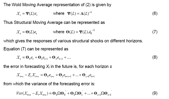 on the basis of this formula, we can compute the share of the total variance of the forecast error for each variable attributable to the variance of each structural shock. The structural impulse response functions (IRF) and structural forecast error variance decomposition (FEVD) emanating from SVAR can be made use of for understanding the association among pricing power, inflation and output at aggregate level as well as at disaggregate level such as for use-based categories and industry groups. This section provides the results of the SVAR analysis. Pricing power, as mentioned earlier, was measured using the operating profit margin (EBITDA to sales ratio). The annualised growth rates of the seasonally adjusted Index of Industrial Production (IIP) and Wholesale Price Index (WPI) were used to represent output growth and inflation, respectively. The analyses were done for Non-Food Manufactured Product (NFMP) group as a whole as well as for the use based categories viz. Basic Goods (BG), Capital Goods (CG), Intermediate Goods (IG), Consumer Durables (CD) and Consumer Non-Durables (CND) separately. Further, analysis was also carried out for seven major industry groups, viz., ‘Textiles’, ‘Coke & Refined Petroleum’, ‘Chemicals’, ‘Non-Metallic Minerals’, ‘Metals and metal products’, ‘Machinery (excluding transport)’ and ‘Transport equipments’. The quarterly data from 2000-01:Q1 to 2011-12:Q3 of 995 companies4 were used for the analysis. The SVARs were estimated controlling for industry concentration, measured using Herfindahl–Hirschman Index (HHI), and business cycles, identified using the Composite Leading Indicator Index for India published by OECD. The lag lengths were identified using Schwarz Bayesian Information Criterion (SBIC). SVARs are characterised by the ordering of variables and the structural restriction metrics. The ordering of the variables was kept common in all the SVARs as pricing power, output and inflation. However, the structural identifications for each of the SVARs were identified and incorporated based on the tests of over-identifying restrictions and, therefore, were different for various SVARs presented in the subsequent sections. The inferences were mainly drawn from the impulse response functions (IRF) and forecast error variance decompositions (FEVD). The detailed results are discussed in the following sections. 6.1 Non-food manufactured products - Results The BIC criteria for the SVAR with pricing power, output and inflation for NFMP as the endogenous variables and HHI for NFMP and the dummy variable representing business cycle as the exogenous variables suggested a lag length of two. The Lagrange multiplier (LM) test of over-identifying restriction suggests that the output affects pricing power contemporaneously, while all other variables affect each other with at least one lag (chi2(2)= 3.639 Prob> chi2 = 0.162). The structural impulse response functions with respect to one standard deviation shocks estimated from the SVAR are presented in Appendix Chart 6.1. The 4-quarter, 8-quarter and 12-quarter ahead structural FEVD are given in Appendix Table 6.1. The FEVD (Appendix Table 6.1) suggests that variation in pricing power in NFMP firms is mainly determined by its own shock (61 per cent in 12-quarter ahead) and shocks from inflation (30 per cent in 12-quarter ahead). Appendix Chart 6.1(b) suggests that a positive shock in inflation significantly reduces the pricing power and its effect lasts to around 4-5 quarters. Even though the response of pricing power to the positive (negative) output shocks is lesser in magnitude, they are found to increase (decrease) the pricing power significantly up to 1-period ahead (Appendix Chart 6.1(a)). Thus, the fall in pricing power of NFMP companies is the result of persistent high inflation and low output. For NFMP, output is more responsive to shocks in pricing power (45 per cent in 12-quarter ahead) than to shocks in inflation (18 per cent in 12-quarter ahead). A negative shock in pricing power significantly reduces the output in one quarter ahead (Appendix Chart 6.1(c)), while high inflation shock reduces the output significantly over a period of 4-5 quarters (Appendix Chart 6.1(d)). Thus, the current fall in the industrial output is partially explained by the fall in the pricing power and the high inflation. The NFMP inflation responds more to its own shocks (73 per cent in 12-quarter ahead) and has a subdued response to the other shocks (Appendix Chart 6.1(e-f)). Even though it is found that a negative shock in output significantly decreases inflation in 1-2 quarters, it explains only 19 per cent of the variation in the inflation. Thus, the observed elevated level of NFMP inflation may be attributed to the low response of inflation to fall in pricing power and lags in the transmission of fall in the industrial output to prices. 6.2 Use based classification groups - Results 6.2.1 Basic goods In case of basic goods, the BIC criteria suggested a lag length of two. The SVAR for basic goods is estimated using the variables pricing power, output and inflation as endogenous variables with HHI for basic goods and the dummy for business cycle as the exogenous variables. The LM test suggests that the output affects pricing power contemporaneously, while all others affect each other with at least one lag (chi2(2)= 0.7642 Prob> chi2 = 0.682). The structural impulse responses of various variables to one standard deviation shocks and the corresponding structural FEVD are given in Appendix Chart 6.2 and Appendix Table 6.2, respectively. Appendix Table 6.2 suggests that the variations in pricing power of manufacturers of basic goods are explained by its own shocks (51 per cent in 12-quarter ahead) and shocks from inflation (43 per cent in 12-quarter ahead). The responses of pricing power to output shocks are short lived and smaller in magnitude (Appendix Chart 6.2(a)). However, high inflation reduces the pricing power significantly in 5-6 quarters (Appendix Chart 6.2(b)). Both output and inflation in case of basic goods are found to be almost non-responsive to the shocks from other variables (Appendix Chart 6.2(c-f)), even though inflation looks like affecting output negatively over a period of one quarter (Appendix Chart 6.2(d)). Thus, it can be concluded that the fall in the pricing power of the basic good manufacturing firms is due to the high inflation and fall in the corresponding industrial output. Further, the shocks in the pricing power affect neither output nor inflation, and have, therefore, only a trivial role in explaining the inflation-output dynamics. 6.2.2 Capital goods For capital goods, the SVAR is estimated with pricing power, output and inflation as endogenous variables with HHI for capital goods and the dummy for business cycle as the exogenous variables. The BIC suggested a lag length of one. As per the LM test all variables affect each other with at least one lag (chi2(3)= 0.8927 Prob> chi2 = 0.827). Appendix Chart 6.3 and Appendix Table 6.3 present the structural impulse response functions to one standard deviation shocks and the structural FEVD for the capital goods, respectively. Appendix Table 6.3 suggests that variation in pricing power and output of the capital goods manufacturers are mostly explained by own shocks. Also, the impulse responses presented in Appendix Charts 6.3(a-d) are found to be insignificant. The inflation in capital goods is partially explained by the shocks in the industrial output. A negative output shock decreases the inflation significantly in 1-2 quarters (Appendix Chart 6.3(f)). This partially explains the low inflation in capital goods. However, the shocks of pricing power seem to be almost insignificant in explaining the inflation (Appendix Chart 6.3(e)). In the case of capital goods, it is likely that inflation is explained by the output shocks, while both pricing power and output seem to be exogenous to the system. 6.2.3 Intermediate goods The estimated identifying restriction of SVAR in case of intermediate goods suggests that inflation affects pricing power contemporaneously, while other effects are with at least one lag (LM chi2(2)= 1.964 Prob> chi2 = 0.375). Following the earlier cases, for intermediate goods, SVAR is estimated with pricing power, output and inflation as endogenous variables and HHI for intermediate goods and the dummy for business cycle as exogenous variables. The BIC criteria suggested a lag length of one. The structural impulse response functions and FEVD for intermediate goods are presented in Appendix Chart 6.4 and Appendix Table 6.4, respectively. Appendix Table 6.4 suggests that in case of intermediate goods, the shocks of pricing power explain 17 per cent variation in output (12 quarters ahead) and 9 per cent variation in inflation (12 quarters ahead). A negative shock of pricing power significantly reduces output in 3-4 quarters (Appendix Chart 6.4(c)) and inflation in 4-5 quarters (Appendix Chart 6.4(e)). The variation in pricing power is partially explained (37 per cent in 12-quarter ahead) by shocks in inflation (Appendix Table 6.4). A positive shock in inflation significantly reduces the pricing power in 3-4 quarters, even though the magnitude seems to be less (Appendix Chart 6.4(b)). However, the output shocks are insignificant in explaining the variation in pricing power of intermediate good producing firms (Appendix Chart 6.4(a)). The positive inflation shocks seem to significantly reduce the industrial output in 3-4 quarters (Appendix Chart 6.4(d)) and a negative shock in output reduces inflation one quarter ahead (Appendix Chart 6.4(f)). Thus, it could be concluded that pricing power holds significant explanatory role in the downward movement of output and inflation in intermediate goods. 6.2.4 Consumer durable goods Similar to earlier cases, SVAR is estimated for consumer durables also with pricing power, output and inflation as endogenous variables; and HHI and the dummy for business cycle as exogenous variables. The estimated lag length as per the BIC criteria was one. LM test for over-identification suggests that inflation affects output contemporaneously, while other effects are with at least one lag (chi2(2)= 0.9814 Prob> chi2 = 0.612). Appendix Chart 6.5 and Appendix Table 6.5 give the structural impulse response functions to one standard deviation shocks and the structural FEVD for consumer durables, respectively. It can be noticed from Appendix Table 6.5 that the shocks in inflation marginally describe the variation in both pricing power (9 per cent in 12-quarter ahead) and output (11 per cent in 12-quarter ahead), even though variation in all the three variables are mostly explained by their own shocks. A positive ‘consumer durables’ inflation shock seems to significantly reduce the pricing power of its firms, 2-3 quarters ahead, though the magnitude is quite marginal (Appendix Chart 6.5(b)). Similarly, a positive inflation shock causes a fall in output almost in the same quarter (Appendix Chart 6.5(d)). All other impulse responses are found to be statistically insignificant (Appendix Chart 6.5). Thus, it could be argued that in the case of consumer durables, inflation shocks seem to drive both output and pricing power marginally. 6.2.5 Consumer non-durable goods The SVAR has been estimated with pricing power, output and inflation as endogenous variables; and HHI and business cycle dummy as exogenous variables. BIC criteria suggested a lag length of one. The test for over-identifying restriction suggests that output affects inflation contemporaneously, while other effects are with at least one lag (chi2(2)= 2.427 Prob> chi2 = 0.297). The structural impulse response functions to one standard deviation shocks and the corresponding structural FEVD are given in Appendix Chart 6.6 and Appendix Table 6.6, respectively. Appendix Table 6.6 suggests that pricing power is almost non-responsive to shocks in output and inflation. Only significant response is that of inflation to output shocks (10 per cent in 12-quarter ahead). The response of inflation to negative output shock is significantly negative in the same quarter (Appendix Chart 6.6(f)). All other impulse responses are found to be statistically insignificant (Appendix Chart 6.6). Thus, falling trend in consumer non-durables output has resulted in some marginal fall in its prices. 6.3 Major industry-wise classification - Results As in the cases of use based categories, for each industry an SVAR is estimated with pricing power, output and inflation as endogenous variables and HHI for the corresponding industry and the dummy for business cycle as exogenous variables. BIC criteria are used to select the optimal lag length. The Lagrange multiplier (LM) test of over-identifying restriction is used to establish the contemporaneous relationships. Appendix Charts 6.7 to 6.13 and Appendix Tables 6.7 to 6.13 give the structural impulse response functions to one standard deviation shocks and the structural FEVDs, respectively, for the select industries. For ‘textiles’ industry, output and inflation seem to affect pricing power, but pricing power does not seem to affect either inflation or output. Inflation and output explain 45 per cent and 29 per cent variation in 12-quarters-ahead pricing power of textile industries, respectively, (Appendix Table 6.7). For ‘coke & refined petroleum’ industry, inflation is found to affect pricing power (21 per cent variation in pricing power in 12 quarters ahead), while the reverse relationship is found to be insignificant (Appendix Table 6.8). However, low pricing power is found to reduce the output (Appendix Chart 6.8). Like in the case of ‘textiles’ industry, for ‘chemicals’ industry also the variation in pricing power is explained by inflation and output. Around 27 per cent variation in 12- quarters-ahead pricing power is explained by inflation and output (Appendix Table 6.9). In case of ‘non-metallic minerals’, pricing power neither determines nor is determined by inflation and output (Appendix Table 6.10 and Appendix Chart 6.10). In case of ‘metals and metal products’, inflation affects pricing power, however, the reverse relationship is not significant (Appendix Chart 6.11b). Shock in inflation causes 26 per cent of the variation in the pricing power 12 quarters ahead. In case of ‘machinery (excluding transport)’ industry, fall in pricing power is reflected in significant fall in output (Appendix Chart 6.12(c)). Around 15 per cent of the variation in output can be explained by the changes in pricing power for the industry. However, inflation is neither found to be significant in explaining or being explained by pricing power. For ‘transport’ industry, fall in pricing power significantly explains fall in output (Appendix Chart 6.13(c)). On the other hand, increase in the output significantly increases the pricing power (Appendix Chart 6.13(a)). However, inflation and pricing power relationship seems to be insignificant. To summarise, at broad industry level, pricing power was not found to have a statistically significant impact on inflation for any industry group other than partially explaining variation in inflation in ‘Metals and metal products’ (13 per cent in 12 quarters ahead) and in ‘Non-Metallic Minerals’ (8 per cent). Hence, the fall in pricing power was not seen, in general, to be reflected in a fall in inflation. Pricing power is found to have a statistically significant impact on output for the groups, viz., ‘Machinery (excluding transport)’, ‘Transport equipments’ (explaining variation by 15 per cent each) and ‘Metals and metal products’ industries (explaining variation by 11 per cent). Hence, it was observed that a decline in pricing power was responded by a fall in output. On the other hand, rise in inflation increased pricing power in ‘Textiles’, ‘Coke and Refined Petroleum’, ‘Chemicals’ and ‘Metals and metal products’. Higher output also caused higher pricing power in ‘Textiles’ and ‘Chemicals’ industries. The dynamics of corporate pricing power and its impact on inflation is well researched area in developed countries. Broad consensus suggests that increased pricing power help pass the surge in input costs to the consumer and hence leads to higher inflation and in falling pricing power the pass-through gets restricted calling for a decline in price level. However, recent trends on these indicators in India were at odds with the general agreement. Data showed that corporate pricing power in India was gradually declining since 2009-10:Q1. Production also fell sharply since 2010-11:Q3. However, WPI inflation has been sticky and remained relatively at a higher level. In this background, this paper examined if the trend in corporate pricing power was getting reflected into the dynamics of inflation and growth based on a SVAR framework, after controlling the impact of market structure and phases of business cycles. Also, the paper examined whether the stickiness of inflation, despite falling pricing power, is a broad-based industry phenomenon. Empirical results indicate that pricing power has a statistically significant and positive impact on output growth in case of non-food manufacturing products. The impact of pricing power on inflation is also positive but relatively subdued. A fall in pricing power was followed by higher and faster decline in production than in inflation. Among use based categories, pricing power displayed significant and positive impact on both inflation and output in the case of intermediate goods only. For other use-based categories, the impact of pricing power on inflation was not statistically significant. This was also observed at broad industry level, except that pricing power partially explained the variation in inflation in ‘metals and metal products’ and in ‘non-metallic minerals’ industries. Finally, it was observed that market structure had a limited role in explaining the nexus among pricing power, inflation and output. In a period of high and persistent inflation, the effect of declining pricing power on reducing inflation has so far been limited. Bottom-line of the corporates is affected by higher input costs and lower output realisation. As the increase in input costs arising from both internal and external shocks was not passed through by increases in selling price, the profit margin of firms declined. Also, due to subdued demand conditions, firms’ response to higher input costs was reflected more in reduced production than in lower prices. @Authors are Assistant Advisers (Angshuman Hait and Joice John) and Directors (Abhiman Das and Anujit Mitra), respectively, in the Department of Statistics and Information Management, Reserve Bank of India, Mumbai. Corresponding author: Angshuman Hait, email. 1Authors are thankful to Smt. Rekha Misra, Director, DEPR, RBI for her valuable inputs. Data used in the paper are sourced from the public domain. Views expressed in the paper are those of the authors and not of the organisation to which they belong. 2Macroeconomic and Monetary Developments, RBI, various issues. 3Based on quarterly data of a sample of 995 companies for the period 2000-01:Q1 to 2011-12:Q3. Data Source: Capitaline database. 4Companies are classified into NFMP, use based categories and industry groups mainly based on the sources of income. Data Source: Capitaline database. References Alvarez L., Dhyne E., Hoeberichts M., Kwapil C., Le Bihan H., Lunnemann P., Martins F., Sabbatini R., Stahl H., Vermeulen P., And Vilmunen, J (2006). Sticky Prices in the Euro Area: A summary of new micro evidence., Journal of the European Economic Association, 4 (2-3): 575-584. Ball, L and S. G. Cecchetti (1988): ‘Imperfect Information and Staggered Price Setting’, American Economic Review, 78 (5), 999-1018. Banerjee, A., Mizen, P., and Russell, B. (2007): ‘Inflation, Relative Price Variability and the Markup: Evidence from the United States and the United Kingdom’, Economic Modelling,24, 82-100. Bils M. and Klenow P. (2004): ‘Some Evidence on the Importance of Sticky Prices’, Journal of Political Economy, 112: 947-985. Blanchard, O. and N. Kiyotaki (1987): ‘Monopolistic competition and the effects of aggregate demand’, American Economic Review, 77: 647-666. Boivin, J., M. P. Giannoni and I. Mihov (2009): ‘Sticky Prices and Monetary Policy: Evidence from Disaggregated US Data’, American Economic Review, 99, 350-384. Campa, J. and L. Goldberg (2005): ‘Exchange-Rate Pass-Through into Import Prices’, Review of Economics and Statistics, 87, 679-90. Choudhri, E. and D. Hakura (2006): ‘Exchange Rate Pass-Through to Domestic Prices: Does the Inflationary Environment Matter?’, Journal of International Money and Finance, 25, 614-639. Devereux, M. B. and J. Yetman (2002): ‘Price Setting and Exchange Rate Pass-Through: Theory and Evidence’, Price Adjustment and Monetary Policy: Bank of Canada Conference Proceedings, 347-371. Devereux, M. B. and Yetman, J. (2003): ‘Predetermined Prices and the Persistent Effects of Money on Output’, Journal of Money, Credit and Banking, 35, 729-741. Etro, F. (2009): Endogenous Market Structures and the Macroeconomy, Springer Fabiani, S., A. Gatulli, and R. Sabbatini (2004): ‘The Pricing Behavior of Italian Firms: New Survey Evidence on Price Stickiness’, European Central Bank Working Paper, No.333. Gagnon, E. (2007): ‘Price Setting During Low and High Inflation: Evidence from Mexico’, Federal Reserve Board International Finance Discussion Paper, 2007-896. Gali, J., and M. Gertler (1999): ‘Inflation Dynamics: A Structural Econometric Analysis’, Journal of Monetary Economics, 44, 195-222. Mankiw N. G. and Romer D (editors 1991): New Keynesian Economics, Vol I, Imperfect competition and sticky prices, MIT Press. Rogoff, Kenneth (2006): ‘Impact of Globalization on Monetary Policy’, The New Geography: Effects and Policy Implications, 2006 Jackson Hole Symposium, Federal Reserve Bank of Kansas City. Taylor, J. B. (2000): ‘Low inflation, pass-through, and the pricing power of firms’, European Economic Review, 44(7), 1389-1408. Taylor, J. B. (2006): ‘The Implications of Globalization for Monetary Policy’, prepared for Academic Consultants Meeting, Federal Reserve Board, September. Topalova P. (2004): ‘Overview of the Indian Corporate Sector: 1989-2002’, IMF Working Papers 04/64, International Monetary Fund. Appendix 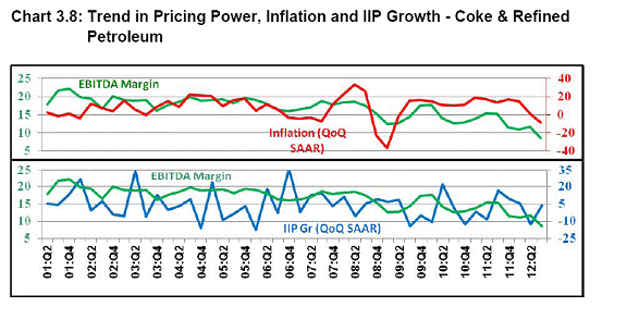 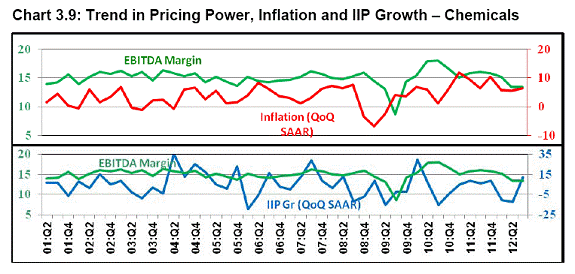 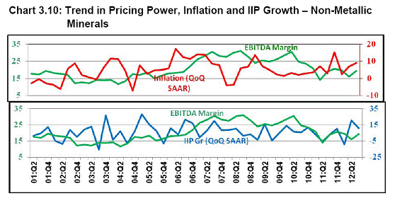 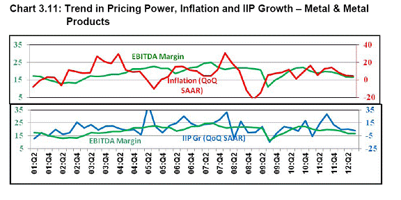 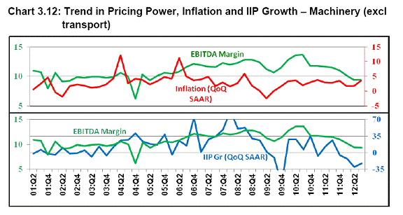 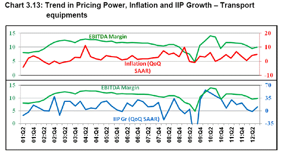 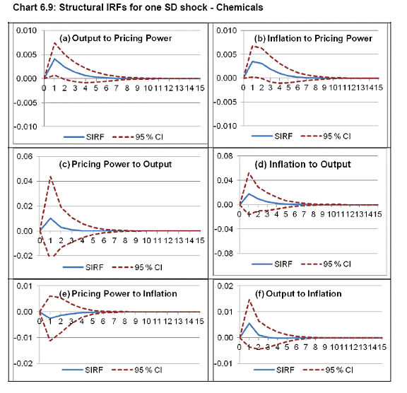 |
Page Last Updated on:


