Macroeconomic Stability Map

The Macroeconomic Stability Map is based on seven sub-indices, each pertaining to a specific area of macroeconomic risk. Each sub-index on macroeconomic risk includes select parameters representing risks in that particular field. These sub-indices have been selected based on their impact on macroeconomic or financial variable such as GDP, inflation, interest rates or asset quality of banks. The seven sub-indices of the overall macroeconomic stability index and their components are briefly described below:

Global Index: The global index is based on output growth of the world economy. A fall in output growth affects overall sentiments for the domestic economy in general and has implications on demand for domestic exports, in particular. Capital flows to the domestic economy are also affected by growth at the global level. Therefore, a fall in output growth is associated with increased risks.

Domestic Growth: The domestic growth index is based on growth of gross domestic product. A fall in growth, usually, creates headwinds for banks’ asset quality, capital flows and over-all macroeconomic stability. Hence, a fall in growth is associated with increased risks.

Inflation: Wholesale Price Index based inflation is used to arrive at the Inflation Index. Increase in inflation reduces purchasing power of individuals and complicates investment decision of corporates. Therefore, an increase in inflation is associated with higher risks.

External Vulnerability Index: The current account deficit (CAD) to GDP ratio, reserves cover of imports and ratio of short term debt to total debt are included in the External Vulnerability Index. Rising CAD and ratio of short term debt to total debt and falling reserves cover of imports depict rising vulnerability.

Fiscal Index: The Fiscal Index is based on fiscal deficit and primary deficit. Higher deficits are associated with higher risk. High government deficit, in general, reduces the resources available to the private sector for investment and also has implications for inflation.

Corporate Index: The health of the corporate sector is captured through profit margin [EBITDA (earnings before interest, tax, depreciation and amortisation) to sales] and the interest coverage ratio [EBIT (earnings before interest, tax) to interest payments]. Lower profit margin and lower interest coverage ratio are associated with higher risks.

Household Index: This index is based on retail non-performing assets, an increase in retail NPAs is associated with higher risk.

Corporate sector Stability Indicator and Map

The Corporate sector Stability Indicator and Map have been constructed using the following method:

Data: The balance sheet data of non-government non-financial public limited companies.

Frequency: Annual (1992-93 to 2013-14). For 2012-13 and 2013-14, the half-yearly balance sheet data is used for the analysis.

Following ratios have been used for the analysis (considering 5 dimensions):

a. Profitability : RoA (Gross Profit/Total Assets) #, Operating Profit/Sales #, Profit After Tax/Sales #;

b. Leverage : Debt/ Assets, Debt/ Equity; (Debt is taken as Total Borrowings)

c. Sustainability : Interest Coverage Ratio (EBIT to interest expenses) #, interest expenses/total expenditure;

d. Liquidity : Quick Assets/ Current Liabilities (quick ratio) #;

e. Turn-Over : Total Sales / Total Assets #.

# Negatively related to risk.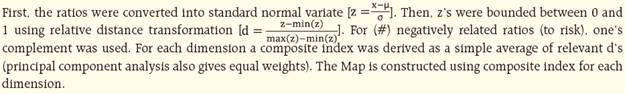

The overall corporate sector stability indicator is a weighted average of 5 dimensions. The weights are obtained using principal component analysis (PCA). The derived weights for 5 dimensions are as follows:

Systemic Liquidity Index

Systemic liquidity in the financial system refers to the liquidity scenario in the banking sector, non-banking financial sector, the corporate sector and the prevailing foreign currency liquidity. Current needs for liquidity are also influenced by the expectations about the availability of funds and their rates in future. The Systemic Liquidity Index (SLI) was constructed using the following four indicators representing various segments of the market:

• Weighted Average Call Rate minus RBI Repo Rate

• 3 month Commercial Paper (CP) Rate minus 3 month Certificate of Deposits (CD) Rate

• 3 month CD Rate minus 3 month Forward Implied Deposit Rate

• Weighted Average Call Rate minus 3 Month Overnight Index Swap (OIS) Rate

The SLI was derived as a simple average of the Standard normal or Variance-equal transformed values of the above mentioned indicators.

Banking Stability Map and Indicator

The Banking Stability Map and Indicator (BSI) present an overall assessment of changes in underlying conditions and risk factors that have a bearing on stability of the banking sector during a period. Following ratios are used for construction of each composite index:

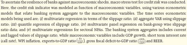
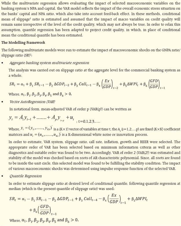
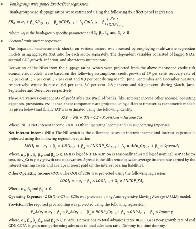
The five composite indices represent the five dimensions of Soundness, Asset-quality, Profitability, Liquidity and Efficiency. Each composite index, representing a dimension of bank functioning, takes values between zero (minimum) and 1 (maximum). Each index is a relative measure during the sample period used for its construction, where a high value means the risk in that dimension is high. Therefore, an increase in the value of the index in any particular dimension indicates an increase in risk in that dimension for that period as compared to other periods. For each ratio used for a dimension, a weighted average for the banking sector is derived, where the weights are the ratio of individual bank asset to total banking system assets. Each index is normalised for the sample period as ‘Ratio-on-a-given-date minus Minimum-value-in-sample-period divided by Maximum-value-in- sample-period minus Minimum-value-in-sample-period’. A composite index of each dimension is calculated as a weighted average of normalised ratios used for that dimension, where the weights are based on the marks assigned for assessment for CAMELS rating. Based on the individual composite index for each dimension, the Banking Stability Indicator is constructed as a simple average of these five composite sub-indices.

Banking Stability Measures (BSMs) – Distress Dependency Analysis

In order to model distress dependency, methodology described by Goodhart and Segoviano (2009) has been followed. First, the banking system has been conceptualised as a portfolio of banks(BIs). Then, the PoD of the individual banks, comprising the portfolio, has been inferred from equity prices. Subsequently, using such PoDs as inputs (exogenous variables) and employing the Consistent Information Multivariate Density Optimizing (CIMDO) methodology (Segoviano, 2006), which is a non-parametric approach based on cross-entropy, the banking system’s portfolio multivariate density (BSMD) have been derived. Lastly, from the BSMD a set of conditional PoDs of specific pairs of BIs, and the banking system’s joint PoD(JPoD) are estimated.

The BSMD and thus, the estimated conditional probabilities and the JPoD, embed the banks’ distress dependency. This captures the linear (correlation) and non-linear dependencies among the BIs in the portfolio, and allows for these to change throughout the economic cycle. These are key advantages over traditional risk models that most of the time incorporate only correlations, and assume that they are constant throughout the economic cycle.

The BSMs uses the following indicators of distress dependency:

Banking Stability Index (BSI): The expected number of banks that could became distressed given that at least one bank has become distressed.

Toxicity Index (TI): The average probability that a bank under distress may cause distress to another bank in the system.

Vulnerability Index (VI): The average probability of a bank coming under distress given distress in other banks in the system.

Network Analysis

Matrix algebra is at the core of network analysis, which is essentially an analysis of bilateral exposures between entities in the financial sector. Each institution’s lending and borrowings with all others in the system are plotted in a square matrix and are then mapped in a network graph. The network model uses various statistical measures to gauge the level of interconnectedness in the system. Some of the most important are as follows:

Connectivity: This is a statistic that measures the extent of links between the nodes relative to all possible links in a complete graph.

Cluster Coefficient: Clustering in networks measures how interconnected each node is. Specifically, there should be an increased probability that two of a node’s neighbours (banks’ counterparties in case of the financial network) are also neighbours themselves. A high clustering coefficient for the network corresponds with high local interconnectedness prevailing in the system.

Shortest Path Length: This gives the average number of directed links between a node and each of the other nodes in the network. Those nodes with the shortest path can be identified as hubs in the system.

In-betweeness centrality: This statistic reports how the shortest path lengths pass through a particular node.

Eigen vector measure of centrality: Eigenvector centrality is a measure of the importance of a node (bank) in a network. It describes how connected a node’s neighbours are and attempts to capture more than just the number of out degrees or direct ‘neighbours’ a node has. The algorithm assigns relative centrality scores to all nodes in the network and a bank’s centrality score is proportional to the sum of the centrality scores of all nodes to which it is connected. In general, for an NxN matrix there will be N different eigen values, for which an eigen vector solution exists. Each bank has a unique eigen value, which indicates its importance in the system. This measure is used in the network analysis to establish the systemic importance of a bank and by far it is the most crucial indicator.

Tiered Network Structures: Typically, financial networks tend to exhibit a tiered structure. A tiered structure is one where different institutions have different degrees or levels of connectivity with others in the network. In the present analysis, the most connected banks (based on their eigen vector measure of centrality) are in the inner most core. Banks are then placed in the mid core, outer core and the periphery (the respective concentric circles around the centre in the diagrams), based on their level of relative connectivity. The range of connectivity of the banks is defined as a ratio of each bank’s in degree and out degree divided by that of the most connected bank. Banks that are ranked in the top 10 percentile of this ratio constitute the inner core. This is followed by a mid core of banks ranked between 90 and 70 percentile and a 3rd tier of banks ranked between 40 and 70 percentile. Banks with connectivity ratio of less than 40 per cent are categorised as the periphery.

Solvency Contagion analysis

The contagion analysis is basically a stress test where the gross loss to the banking system owing to a domino effect of one or more bank failing is ascertained. We follow the round by round or sequential algorithm for simulating contagion that is now well known from Furfine (2003). Starting with a trigger bank ‘i’ that fails at time 0, we denote the set of banks that go into distress at each round or iteration by Dq, q= 1,2, …For this analysis, a bank is considered to be in distress when its core CRAR goes below 6 per cent. The net receivables have been considered as loss for the receiving bank.

Liquidity Contagion analysis

While the solvency contagion analysis assesses potential loss to the system owing to failure of a net borrower, liquidity contagion estimates potential loss to the system due to the failure of a net lender. The analysis is conducted on gross exposures between banks. The exposures include fund based and derivatives. The basic assumption for the analysis is that a bank will initially dip into its liquidity reserves or buffers to tide over a liquidity stress caused by the failure of a large net lender. The items considered under liquidity reserves are (a) excess CRR balance; (b) excess SLR balance; (c) available marginal standing facility and (d) available export credit refinance. If a bank is able to meet the stress with the liquidity buffers alone, then there is no further contagion.

However, if the liquidity buffers alone are not sufficient, then a bank will call in all loans that are ‘callable’, resulting in a contagion. For the analysis only short term assets like money lent in the call market and other very short term loans are taken as callable. Following this, a bank may survive or may be liquidated. In this case there might be instances where a bank may survive by calling in loans, but in turn might propagate a further contagion causing other banks to come under duress. The second assumption used is that when a bank is liquidated, the funds lent by the bank are called in on a gross basis, whereas when a bank calls in a short term loan without being liquidated, the loan is called in on a net basis (on the assumption that the counterparty is likely to first reduce its short term lending against the same counterparty).

Estimation of Losses: Expected Loss, Unexpected Loss and Expected Shortfall of SCBs

The following standard definitions have been used for estimation of these losses:

Expected Loss (EL) : The EL is the average credit loss that the banking system expects from their credit exposure.

Unexpected Loss (UL) : The UL at 100(1-α) per cent-level of significance is the loss that may occur at the α-quantile of the loss distribution.

Expected Shortfall (ES) : When the distributions of loss (Z) are continuous, expected shortfall at the 100(1-α) per cent confidence level ( ESα (Z) ) is defined as, ESα (Z) = E[Z – Z≥ VaRα (Z)]. Hence, Expected shortfall is the conditional expectation of loss given that the loss is beyond the VaR level.

These losses were estimated as: Loss = PD X LGD X EAD

Where, EAD = Exposure at Default, is the total advances of the banking system. EAD includes only on-balance sheet items as PD was derived only for on balance sheet exposures.

LGD = Loss Given Default. Under baseline scenario, the average LGD was taken as 60 per cent as per the RBI guidelines on ‘Capital Adequacy – The IRB Approach to Calculate Capital Requirement for Credit Risk’. LGD was taken at 65 per cent and 70 per cent under medium and severe macroeconomic conditions, respectively.

PD = Probability of Default. PD was defined as gross non-performing advances to total advances ratio. Because of unavailability of data on number of default accounts, the size of default accounts (i.e. NPA amount) has been used for derivation of PDs.

The above losses viz., EL, UL and ES, were estimated by using a simulated PD distribution. As a first step; an empirical distribution of the PD was estimated using Kernel Density Estimate, second; using the empirically estimated probability density function, 20000 random numbers were drawn based on Monte Carlo Simulation and finally, for calculation of expected loss, unexpected loss and expected shortfall, PDs were taken as average PD, 99.9 per cent VaR of PD and average PD beyond 99.9 per cent loss region, respectively.

Macro Stress Testing

Income Tax: The required income tax was taken as 32 per cent of the profit before tax, which is based on the past trend of ratio of income tax to profit before tax.

Finally, impact on CRAR was estimated based on the PAT estimated as mentioned above. RWA growth is assumed as 17.5 per cent. The regulatory capital growth is assumed to remain at the minimum by assuming minimum mandated transfer of 25 per cent of the profit to the reserves account. The projected values of the ratio of the non-performing advances were translated into capital ratios using the “balance sheet approach”, by which capital in the balance sheet is affected via the provisions and net profits.

Single Factor Sensitivity Analysis – Stress Testing

As a part of quarterly surveillance, stress tests are conducted covering credit risk, interest rate risk, liquidity risk etc. Resilience of the commercial banks in response to these shocks is studied. The analysis is done on individual scheduled commercial bank as well as on the aggregated-system.

Credit Risk

To ascertain the resilience of banks, the credit portfolio was given a shock by increasing NPA levels, for the entire portfolio. For testing the credit concentration risk, default of the top individual borrower(s) and the largest group borrower was assumed. The analysis was carried out both at the aggregate level as well as at the individual bank level, based on supervisory data as on September 30, 2013. The assumed increase in NPAs was distributed across sub-standard, doubtful and loss categories in the same proportion as prevailing in the existing stock of NPAs. The provisioning norms used for these stress tests were based on existing average prescribed provisioning for different asset categories. The provisioning requirements were taken as 25, 75 and 100 per cent for sub-standard, doubtful and loss advances, respectively. These norms were applied on the additional NPAs, calculated under a stress-scenario. As a result of assumed increase in NPAs, loss of income on the additional NPAs for one quarter was also included in total losses in addition to additional provisioning requirements. The estimated provisioning requirements so derived were deduced from banks’ capital and stressed capital adequacy ratios were derived.

Interest rate risk

The fall in value of the portfolio or income losses due to the shifting of INR yield curve are accounted for the total loss of the banks because of the assumed shock. The estimated total losses so derived were reduced from the banks’ capital.

For interest rate risk in the banking book, Duration Analysis approach was considered, for computation of the valuation impact (portfolio losses) on the investment portfolio. The portfolio losses on investments were calculated for each time bucket based on the applied shocks. The resultant losses/gains were used to derive the impacted CRAR. The valuation impact for the tests on banking book was calculated under the assumption that the HTM portfolio would be marked to market. In a separate exercise for interest rate shocks in trading book, the valuation losses were calculated for each time bucket on the interest bearing assets using duration approach.

Liquidity Risk

The aim of liquidity stress tests is to assess the ability of a bank to withstand unexpected liquidity drain without taking recourse to any outside liquidity support. The analysis is done as at end-September 2013. Various scenarios depict different proportions (depending on the type of deposits) of unexpected deposit withdrawals on account of sudden loss of depositors’ confidence and assess the adequacy of liquid assets available to fund them.

Assumptions in the liquidity stress test are as follows:

• It is assumed that banks would meet stressed withdrawal of deposits through sale of liquid assets only.

• The sale of investments is done with a hair cut of 10 per cent of their market value.

• The stress test is done on a static mode.

Stress Testing of Derivatives Portfolio of Select Banks

The stress testing exercise focused on the derivatives portfolio of a representative sample set of top 24 banks in terms of notional value of derivatives portfolio. Each bank in the sample was asked to assess the impact of stress conditions on their respective derivatives portfolios.

In case of domestic banks, the derivatives portfolio of both domestic and overseas operations was included. In case of foreign banks, only the domestic (i.e. Indian) position was considered for the exercise. For derivatives trade where hedge effectiveness was established was exempted from the stress tests, while all other trades were included.

The stress scenarios incorporated four sensitivity tests consisting of the spot USD/INR rate and domestic interest rates as parameters

Scheduled Urban Co-operative Banks

Credit Risk

Stress tests on credit risk were conducted on Scheduled Urban Co-operative Banks (SUCBs) using their asset portfolio as at end-September 2013. The tests were based on single factor sensitivity analysis. The impact on CRAR was studied under four different scenarios. The assumed scenarios were as under:

• Scenario I: 50 per cent increase in GNPA (classified into sub-standard advances).

• Scenario II: 50 per cent increase in GNPA (classified into loss advances).

• Scenario III: 100 per cent increase in GNPA (classified into sub-standard advances).

• Scenario IV: 100 per cent increase in GNPA (classified into loss advances).

Liquidity Risk

Liquidity stress test based on cash flow basis in 1-28 days time bucket was also conducted, where mismatch [negative gap (cash inflow less than cash outflow)] exceeding 20 per cent of outflow was considered stressful.

• Scenario I: Cash out flows in 1-28 days time bucket goes up by 50 per cent (no change in cash inflows).

• Scenario II: Cash out flows in 1-28 days time bucket goes up by 100 per cent (no change in cash inflows).

Non-Banking Financial Companies (ND-SI)

Credit Risk

Stress tests on credit risk were conducted on Non-Banking Financial Companies (includes both Deposits Taking and Non-Deposit taking and Systemically Important) using their asset portfolio as at end-September 2013. The tests were based on single factor sensitivity analysis. The impact on CRAR was studied under two different scenarios;

• Scenario I: GNPA increased two times from the current level.

• Scenario II: GNPA increased 5 times from the current level.

The assumed increase in NPAs was distributed across sub-standard, doubtful and loss categories in the same proportion as prevailing in the existing stock of NPAs. The additional provisioning requirement was adjusted from the current capital position. The stress was conducted at individual NBFCs as well as at an aggregate level.

¹ Slippages are the fresh accretion to NPAs during a period. Slippage Ratio = Fresh NPAs / Standard Advances at the beginning of period.

² Slippage ratio, exports/GDP, and the call rate are seasonally adjusted.