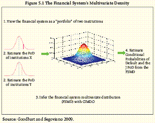
The relevance of systemic risk in the financial sector has been underscored by the global financial crisis. It is the risk of disruption to financial services that is (i) caused by an impairment of all or parts of the financial system and (ii) has the potential to have serious negative consequences for the real economy. The importance of the measurement of systemic risk in the financial sector is growing significantly.The importance of the measurement of systemic risk in the financial sector is growing significantly. In fact, measuring aggregate financial sector risk, i.e. the occurrence of a systemic event which would have severe implications not only on the stability of the financial system but also on the economy at large, has become one of the key area of research worldwide. Systemic risk measurement is clearly in its early stages of evolution. There are various approaches for the measurement of systemic risk and financial statement-based measures, exposure-based network models and measures based on capital market data are the prominent ones. However, these measures are not fully consistent and over-reliance on one measure may lead to biased inference. This requires a comprehensive approach to arrive at a conclusive decision by considering measures achieved through different methodologies.

Monitoring of financial stability indicators and conducting stress-testing exercises are the main practical approaches of macroprudential oversight. Stress testing is forward looking and can be tailored to the specifics of a given financial system. Stress tests are meant to evaluate the resilience of individual financial institutions and of financial sectors to highly adverse but plausible events. They are used to quantify vulnerabilities, both from a microprudential perspective within Supervisory Risk Assessments, where financial institutions are analysed individually, and from a macroprudential perspective within Financial Stability Analyses, where the resilience of the entire financial sector to adverse macroeconomic shocks is tested.

5.1 In this report, the stability of banks has been studied through the Joint Probability of Distress (JPoD) and the Banking Stability Index (BSI), which takes into account the impact of one bank on others through direct or indirect links. Further, the resilience of the commercial banks in respect of credit, interest rate and liquidity risks were also studied through stress testing by imparting extreme but plausible shocks. A stress test on the projected balance sheet was undertaken for the commercial banking system which included both baseline and stressed scenarios. The credit risk of the commercial banks has also been tested through macro-stress test models, which link measures of credit risk to the macroeconomic variables using multivariate regression equation as well as a Vector Autoregressive (VAR) approach. Single factor sensitivity analysis of credit risk of scheduled urban co-operative banks and non-banking financial companies were also conducted. The methodologies used in these stress tests are described in the Annex.

Banking Stability Measures¹

5.2 During times of distress, the fortunes of banks typically decline concurrently through direct links or through indirect links which include mark-to-market asset values, interbank lending and information asymmetries. This section models distress dependencies as the financial system is conceptualised as a portfolio of a specific group of banks (Segoviano and Goodhart, 2009)². In particular, the Banking System’s Portfolio Multivariate Density (BSMD), which characterises both the individual and joint asset value movements of the portfolio of banks, is recovered from the empirically observed Probabilities of Distress (PoDs) of the banks under analysis (Box 5.1 CIMDO-Approach)³. The BSMD embeds banks’ distress dependence structure, which captures banks’ linear (correlations) and non-linear distress dependence, and their changes throughout the economic cycle, reflecting the fact that dependence increases in periods of distress. By recovering the (entire) portfolio multivariate density that describes the system; the CIMDO-approach allows to analyse financial stability from three different, yet, complementary perspectives; viz., (i) common distress of the financial institutions in a system, (ii) distress between specific institutions, and (iii) distress in the system associated by distress in a specific institution. The possibility to analyse financial stability from complementary perspectives represents a key advantage over the analysis of any single perspective by providing policy makers with an enhanced set of information that might be useful to identify how risks are evolving, and where contagion might most easily develop. This methodology also offers great flexibility for implementation, since the PoDs of individual bank represent the input variables, which can be estimated using alternative approaches⁴.

Box 5.1. CIMDO-Approach

In modeling distress dependence, methodology described by Goodhart and Segoviano (2009) has been followed. First, the financial system has been conceptualised as a portfolio of institutions (FIs). Then, the PoD of the individual institutions, comprising the portfolio, has been inferred from equity prices (Figure 5.1). Subsequently, using as inputs (exogenous variables) such PoDs, and employing the Consistent Information Multivariate Density Optimizing (CIMDO) methodology (Segoviano, 2006), a novel non-parametric approach based on cross-entropy, the financial system’s portfolio multivariate density (FSMD) have been derived. Lastly, from the FSMD a set of conditional PoDs of specific pairs of FIs, and the financial system’s JPoD are estimated.

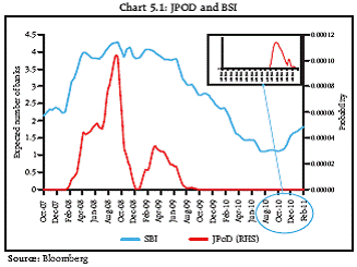
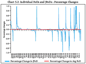
The FSMD and thus, the estimated conditional probabilities and the JPoD, embed the institutions’ distress dependence. This captures the linear (correlation) and non-linear dependencies among the FIs in the portfolio, and allows for these to change throughout the economic cycle. These are key advantages over traditional risk models that most of the time incorporate only correlations, and assume that they are constant throughout the economic cycle.

The distress dependence structure embedded in the FSMD is characterised by the CIMDO-copula (Segoviano, 2006). The structure of linear and nonlinear dependencies among the assets in a portfolio can be represented by copula functions. This approach infers copulas directly from the joint movement of individual PoDs. This is in comparison to parametric copula approaches, in which parametric copula functions have to be chosen and calibrated explicitly— usually a difficult task, especially under data constraints.

Common distress in the system: JPoD and BSI

Distress dependence down from crisis period, but cropping up again

5.3 For the first perspective, two indicators, the Joint Probability of Distress (JPoD) and the Banking Stability Index (BSI) have been used⁵. The JPoD represents the probability of all the banks in the system (portfolio) becoming distressed. Whereas, BSI reflects the expected number of banks becoming distressed given that at least one bank has become distressed. The JPoD and BSI were estimated for the period from October 2007 up to February 2011 and are presented in Chart 5.1. It may be observed that the expected number of banks (out of the sample of 20) which was under distress was 4 during the crisis has declined to 1 by the last quarter of 2010. But, it has again increased to 2 during the first quarter of 2011. Distress dependence across banks rises during times of crisis, indicating that systemic risks, as implied by the JPoD and the BSI, rise faster than individual risks. The JPoD and the BSI not only take account of individual banks’ probabilities of distress, but these measures also embed banks’ distress dependence. Therefore, these measures may experience larger and nonlinear increases than those experienced by the probabilities of distress (PoDs) of individual banks. Chart 5.2 shows that daily percentage changes of the JPoD are larger than daily percentage changes of the average of individual PoDs. This empirical fact provides evidence that in times of distress, not only do individual PoDs increase, but so does distress dependence. Therefore, measures of financial stability that are based on averages or indices may not be able to indicate the proper estimates.

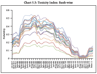
Distress between specific institutions

5.4 To analyse stability from the second perspective, a set of pair wise conditional probabilities of distress, have been estimated which are described as a Distress Dependence (DiDe) Matrix. The matrix shows the conditional probability of distress of the bank on a row given that the bank on the column falls in distress. The distress dependences are estimated daily. The distress dependency of a bank is analysed through a Toxicity Index which shows that if that bank is in distress what is the expected probability of it causing distress to another bank in the system.

5.5 The distress dependence across major banks increased substantially (Chart 5.3). For the purpose of comparative analysis, October 10, 2007 and September 20, 2008 have been chosen to evaluate how conditional probabilities of distress evolved from an initial stage of the crisis to the aftermath of Lehman Brothers filing for bankruptcy. On average, if any of the banks fell into distress, the average probability of the other banks being distressed increased from 17 percent on October 10, 2007 to 42 percent on September 20, 2008. Moreover, on an average, distress of a specific bank would have caused the highest distress in the system (toxicity) in October 2007 (29 percent) while in September 2008, it would have been another bank that would have caused the highest toxicity (53 percent).

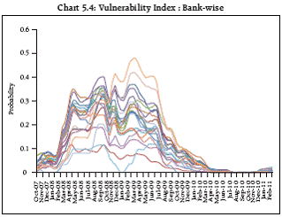
5.6 From the DiDe matrix, Vulnerability Index (VI), which quantifies the vulnerability of a bank given distress in the other banks in the system⁶, is derived and presented in Chart 5.4. It may be observed from the chart that the vulnerability of banks was high during the recent financial crisis but declined substantially during the subsequent period. Whereas, during the recent period, a marginal increase in vulnerability has been observed.

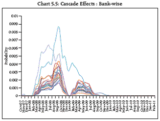
Even though distress dependence does not imply causality, these results show that the analysis of distress dependence, even several weeks prior to a distress event, can provide useful insights into how distress in a specific institution can affect other institutions and ultimately the stability of the system.

Cascade Effects

5.7 To analyse stability from the third perspective, the Probability of Cascade Effects (PCE) has been used. This represents the likelihood that one or more banks in the system become distressed, given a specific bank becomes distressed. Thus, this indicator is useful to quantify the systemic importance of a specific bank, if it becomes distressed, signaling the possible “domino” effects of that specific institution. Chart 5.5 shows bank-wise indicator across time for select banks. It is clear from the chart that cascade effect of select banks declined substantially after the crisis period.

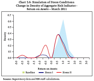
Credit Risk

Under stress conditions, profits lowered but not much pressure on capital adequacy

5.8 A scenario analysis was undertaken for testing the credit risk using a balance sheet approach. The balance sheet and profit and loss account of the banks were projected for March 2012. Along with an enhancement in the provisioning requirements as proposed in the Monetary Policy Statement for the year 2011-12, the scenario framework also assumed that 30 per cent of restructured standard assets would turn into NPAs. Plausible shocks were administered on the projected financials of the banks to gauge their impact and the resilience of the system. The analysis was carried out both at the aggregate level as well as at the individual bank level based on supervisory data for March 2011.

5.9 Under the stress condition, profitability of banks were adversely affected (Chart 5.6). The Return on Assets (RoA) density function under stress conditions shifted towards negative values indicating more and more banks unable to earn positive returns under the assumed stress conditions. However, the banking system was able to withstand an adverse NPA shock reasonably with their capital fund (Table 5.1). At end-March 2012, the projected system level CRAR remained at 11.27 per cent, while at individual bank level, except for one small bank, all banks maintained the CRAR above 9 per cent. The percentage of gross NPAs to total advances increased to 2.92 per cent as at end-March 2012 from 2.34 per cent as at end-March 2011 mainly on account of assumption of 30 per cent of restructured standard assets turning into NPAs. Under the most stringent credit quality shock of 150 per cent on the baseline, when the NPA level increased to 6.33 per cent, the system CRAR stood at 9.33 per cent. However, the system level CRAR was adversely affected under very extreme deterioration of asset quality, when the NPA rose by 168 per cent, impacting 25 banks having a share of 46.00 per cent in total assets, whose CRAR fell below 9 per cent.

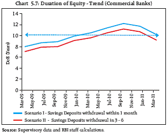
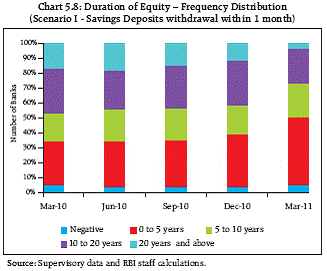
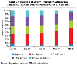
Interest Rate Risk - Duration of Equity

DoE at elevated level… Not much negative impact on capital, though

5.10 Duration of Equity (DoE) of commercial banks, which shows extent of erosion in capital due to unit increase in interest rates, continued to remain at an elevated level, albeit a short detour, in recent quarters. This suggests active involvement of banks in managing interest rate risks (Chart 5.7). Further, the distribution of DoE under the two scenarios showing movement of banks from higher duration to lower duration time buckets (Charts 5.8 and 5.9) indicates that the banks’ vulnerability to increase in interest rate will not be very significant under normal conditions. On the balance, need for maintaining a lower level of DoE on sustained basis, may be a possible recourse available to the banks.

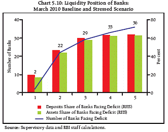
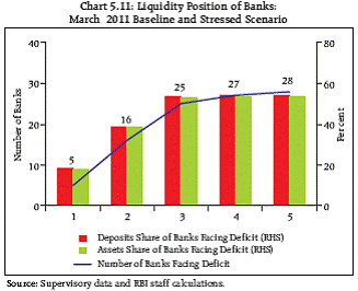
Liquidity Risk

Lurking liquidity constraints under stringent stress scenarios while no potential strains at hand

5.11 Liquidity stress tests showed that a few banks did not have adequate liquid assets to meet the withdrawals on the first day itself. The number of such banks increased in March 2011 as compared to March 2010. However, the total number of banks unable to withstand the stress scenario at the end of five days was higher in March 2010 (Charts 5.10 and 5.11) indicating a slight improvement of the position under the liquidity stress tests relative to the previous assessment.

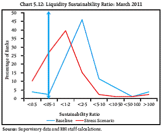
5.12 The analysis of liquidity of banks for the quarter March 2011 is also done using Liquidity Sustainability Ratio (LSR) which has been defined as (Liquid Assets/ Outflows in 1-14 days time bucket). Under the stress scenario the outflow is assumed to be increased by a factor of 3. In the baseline scenario only 5 banks had LSR less than 1, which increased to 29 banks under the stress scenario. These banks have to meet the outflow through purchased liquidity, which is expensive. Further, under stress situation, with falling confidence, these banks may face extreme liquidity constraints showing signs of vulnerability for the system (Chart 5.12).

Macro-stress tests: Multivariate Regression⁷

Impact of macroeconomic shocks on banking sector not substantial

5.13 The model based approach for the macro-stress test used a multivariate equation which directly links macroeconomic variables to measures of bank performance. The impact of macro variables on nonperforming advances (NPAs), defined as ratio of gross non-performing advances to total advances, was estimated. The NPA-ratio was observed to be strongly auto-correlated. Though related negatively to agricultural and industrial GDP growth rates, it was seen to have positive relationship with short term nominal interest rate and inversely related to export-to-GDP ratio.

5.14 The model was used to forecast NPAs under the baseline as well as stress scenarios, with a stress test risk horizon of one year. The baseline and stress scenarios were constructed based on assumptions detailed in Tables 5.2 and 5.3.

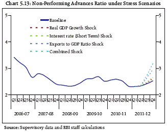
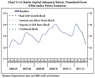
5.15 The results (Charts 5.13 and 5.14) show that impact of select macroeconomic variables, in the aforesaid macro-stress testing model, are not very significant. The results, under different scenarios, therefore, suggest that the macroeconomic shocks would not substantially threaten the Indian banking sector.

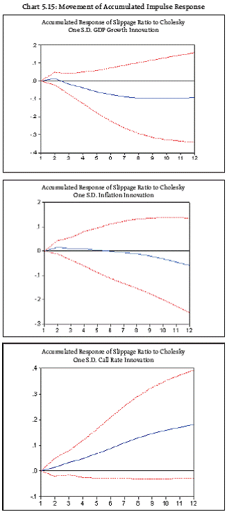
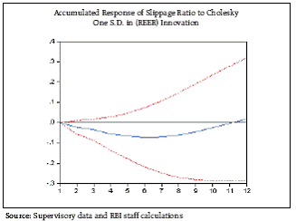
Macro-stress tests: VAR Model

With interest rates rising, loan losses may follow suit

5.16 A vast body of literature endorses the fact that changes in macroeconomic conditions of any economy do impact banks’ performance, simultaneously or with a lag. It is also possible that the feedback effects of bank instability on real economic activity could amplify the fluctuations especially during recessions. Therefore, in order to judge the resilience of banking sector to various macroeconomic shocks, Vector Autoregressive (VAR) approach has been adopted. The advantage of VAR model is that, it allows to fully capture the interaction among macroeconomic variables and banks’ stability variable. It also captures the entailed feedback effect.

5.17 This exercise has been done using quarterly data since Q1 of 2001-02 to Q4 of 2010-11 on four macroeconomic variables, namely, GDP growth, inflation based on WPI, call money rate and Real Effective Exchange Rate (REER). Further, to reflect banks’ stability, slippage ratio has been considered.

5.18 Based on the estimated VAR(2), the impulse response was generated. The accumulated response of slippage ratio to innovation in growth rate, inflation, call rate and REER is presented in the Chart 5.15. It is observed that one standard deviation (positive) shock to GDP growth will lead to decline in slippage ratio by 0.10 over a period of nine quarters. Though inflation has positive impact on slippage ratio, this impact was observed to be marginal: one standard deviation (positive) shock in inflation would raise the slippage ratio by 0.02 over two quarters. However, interest rate has not only significant impact on slippage ratio, such impact was also seen to be long lasting. One standard deviation (positive) shock in call rate tended to raise slippage ratio by 0.22 over twelve quarter. Whereas, REER had negative impact on slippage ratio, one standard deviation (positive) shock in REER prompted a fall in slippage ratio by 0.07 over six quarters.

Under stress scenarios of lower GDP growth and higher rates of inflation & interest, NPA ratio would increase further

5.19 Based on the impulse response function of the VAR, Gross NPA ratio was estimated under two stress scenarios and is presented in Table 5.4.

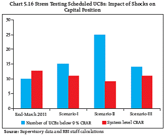
Scenario I: GDP growth will decline by 150 basis points (negative shock), WPI based inflation will increase by 150 basis points, interest rate will increase by 100 basis points and rupee will depreciate by 10 per cent (negative shock).

Scenario II: GDP growth will decline by 250 basis points (negative shock), WPI based inflation will increase by 250 basis points, interest rate will increase by 200 basis points and rupee will depreciate by 20 per cent (negative shock).

The results indicated that under the baseline scenario, the Gross NPA ratio is expected to be around 2.95 per cent by March 2012 a rise of 64 basis points over the March 2011 figures, while under the extreme stress conditions, this ratio is projected to rise further to around 3.31 per cent.

5.20 It is observed from impulse response and variance decomposition that among all the four selected macroeconomic variables, viz., GDP growth, inflation, interest rate and exchange rate; interest rate has the highest (negative) impact on slippage ratio of the banks. This may have profound implications at this point of time considering the fact that stubborn inflation rate would prompt interest rates to keep on hardening impacting adversely asset quality of banks.

Urban Co-operative Banks

Credit risk not alarming

5.21 Stress tests on credit risk were conducted on Scheduled Urban Co-operative Banks (SUCBs) using their asset portfolio as at end-March 2011. The results are based on single factor sensitivity analysis. Impact of shocks on CRAR was tested under three different scenarios, which assumes (i) increase in NPA ratio by 50 per cent, (ii) increase in NPA ratio by 100 per cent and (iii) no profit earned by banks (Chart 5.16). It is observed that SUCBs could withstand shocks assumed under scenarios I and III easily. However, the sector would come under some stress under the stringent scenario II.

Non-Banking Financial Companies (ND-SI)

Impact of credit risk on capital not very significant

5.22 A stress test on credit risk for NBFC-ND-SI sector was carried out as on March 2010 under two scenarios (i) Gross NPA increased two times and (ii) Gross NPA increased 5 times from current level. It was observed that first scenario did not warrant any additional provision as the sector had excess provision towards NPAs while in the second scenario, it was observed that even though there was shortfall in provisioning the impact on CRAR was negligible as the sector had a higher level of CRAR of 37.1 per cent as against the required level of 12 per cent.

Concluding Remarks

5.23 Distress dependence across banks rises during times of crisis, indicating that systemic risks, as implied by the JPoD and the BSI, rise faster than individual risks. The distress dependence across major banks increased substantially during the global crisis period. The vulnerability of banks was high during the recent financial crisis but declined substantially during the subsequent period. However, during the recent period, a marginal increase in vulnerability has been observed for Indian banks. The cascade indicator quantifies the systemic importance of a specific bank, if it becomes distressed, signaling the possible “domino” effects of that specific institution. The cascade effect of select banks declined substantially after the crisis period.

5.24 Projected balance sheet analysis indicated that under stressful conditions, profitability of commercial banks may get adversely affected. However, the banking system would be able to withstand an adverse NPA shock reasonably easily because of its high capital levels. The interest rate risk through the Duration of Equity (DoE) method showed that the DoE continued to remain at elevated level, with an improvement in recent quarters, suggesting active involvement of banks in managing interest rate risks. Regarding liquidity stress test, under severe stress situation, when market sentiment is poor, some banks may face extreme liquidity constrain and may show a sign of vulnerability. The results of macrostress test under different scenarios suggested that macroeconomic shocks would not substantially threaten the Indian banking sector. The VAR methodology indicated that in the current environment of stubborn inflation, which may prompt the interest to be hardened, the asset quality of banks may be impacted adversely. The credit risk stress tests on NBFC-ND-SI and scheduled UCBs revealed that the impact on CRAR under different scenarios would not be alarming.

¹ This model for Indian banking system has been developed by Mr. Miguel A. Segoviano, CNBV (Comisión Nacional Bancaria y de Valores : Mexican financial Regulatory-Supervisory Agency).

² In this study twenty scheduled commercial banks have been considered comprising about seventy five per cent of total assets of commercial banks.

³ The BSMD is recovered using the Consistent Information Multivariate Density Optimizing (CIMDO) methodology Segoviano Miguel ( 2006) which is a non-parametric framework based on the cross-entropy approach (Kullback, 1959). Segoviano Miguel (2006): Consistent Information Multivariate Density Optimizing Methodology, Financial Markets Group, London School of Economics, Discussion Paper 557.

⁴ There are also other methodologies to estimate probabilities of distress (PoDs), notably using CAMEL ratings, Merton approach, etc. The PoDs for banks were estimated from their equity return distributions. Under this approach, first, banks’ historical distributions of equity returns are estimated. Then, the probability of returns falling under the historical worse .05 per cent of the cases (99.5 VaR) is quantified. Therefore, the PoD of a specific bank represents the probability that the bank’s equity return would fall in the worse.05 historical percentile.

⁵ See Segoviano and Goodhart (2009): Banking Stability Measures. IMF.WP/09/4 for definitions.

⁶ For example for a system with three FIs, the VI for the financial institution A would be estimated as P(A/B)*P(B) + P(A/C)*P(C)

⁷ i) Cihak, M. (2007). Introduction to Applied Stress Testing. IMF Working Paper WP/07/59.
ii) Juraj Zemen, Pavol Jurca (2008): Macro Stress Testing of Slovak Banking Sector. Working Paper 1/2008. National Bank of Slovakia.
iii) Marco, Sorge (2004). Stress-testing financial systems: an overview of current methodologies. BIS Working Papers No 165.
iv) Philippines: Financial System Stability Assessment Update (2010). IMF Country Report No. 10/90. April 2010.