 IST,
IST,
Chapter V : Systemic Risk Assessment
The Systemic Risk Survey, the second in the series conducted by the Reserve Bank, revealed that financial sector stakeholders continued to repose confidence in the stability of the domestic financial system. The level of confidence, however, seems to have diminished since the previous Survey. Market volatility emerges as the chief concern of respondents along with the risks associated with high levels of fiscal and current account deficits. Policy risk (including perceived slowdown in policy making) also emerges more prominently in the current Survey. The Systemic Liquidity Indicator pointed to some stress in liquidity conditions during March and April as the banking system’s liquidity deficit remained consistently in excess of the Reserve Bank’s stated comfort zone. Some concerns emerged from the rising trend of short term borrowings of banks especially as the systemic importance of some banks has increased over the last one year. Insurance companies and Mutual Funds (MFs) remain vulnerable to contagion risks from the banking system while banks continue to rely on these segments for their funding needs. The results of a series of stress tests carried out to study the impact of various adverse macro-financial shocks on the health of banks showed that the banking system remained resilient even under extreme stress scenarios. An assessment of the stability of the banking system conducted through a series of Banking Stability Measures (BSMs) indicated that distress dependencies amongst banks had increased in recent periods but remained well below the levels observed during the global financial crisis in 2008-09. Systemic Risk Survey 5.1 The first Systemic Risk Survey was conducted by the Reserve Bank in October 2011 to capture the views of market participants and other stakeholders on the aggregate risks facing the financial system. The second Survey was conducted in April 2012.
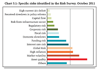
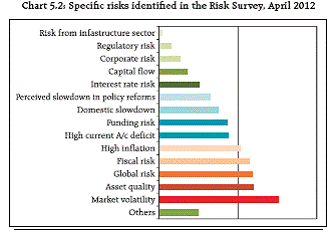
Volatility in the financial markets voted the primary concern 5.2 The second Survey reveals that stakeholders perceive volatility in the markets as the single most important risk facing the financial system, followed by global and fiscal risks. Asset quality, which was perceived to be the most significant risk in the previous Survey, emerged as the second most significant risk in this Survey. Respondents felt that risks from the twin deficits and from perceived slowdown in policy making have increased sharply since the last Survey (Chart 5.1 and Chart 5.2)1.
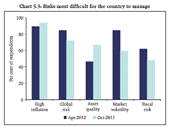
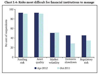
Risks emanating from inflation most difficult for the country to manage 5.3 Survey respondents felt that managing inflation continues to be the biggest challenge for the country (Chart 5.3). For Survey respondents from financial institutions, asset quality and funding risks remained the most difficult to manage (Chart 5.4).
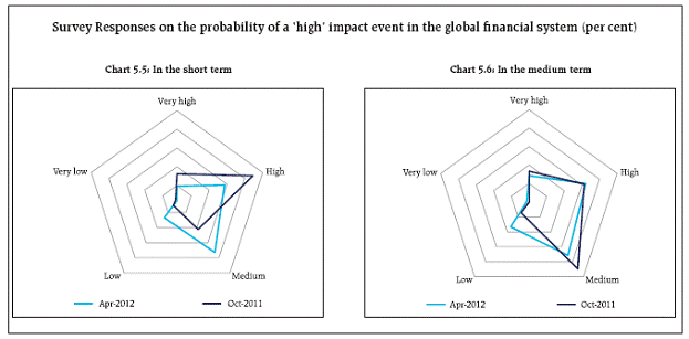
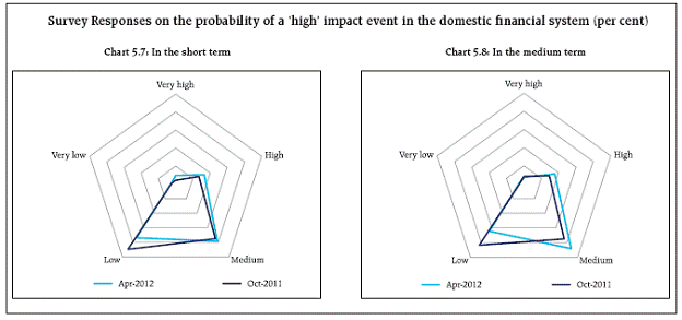
Perceived risks to domestic financial stability increased 5.4 About 43 per cent of the respondents felt that the probability of a systemic event impacting the global financial system in the short term is ‘high’, while 46 per cent thought that the probability was ‘high’ in the medium term. This represents a departure from the earlier Survey where over 60 per cent of the participants felt that the probability of a systemic event impacting the global financial system in the short run was ‘high’. Respondents felt that the risks to the stability of the domestic financial system in the medium term had increased (Charts 5.5 to Chart 5.8).
5.5 The Survey result also revealed that an increasing number of respondents felt that the impact of a global systemic event on the domestic financial system will be ‘high’ (Table 5.1).
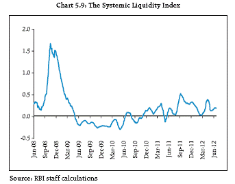
5.6 The Survey respondents continued to repose confidence in the stability of the domestic financial system with 25 per cent of the respondents being ‘very confident’ in the stability of the domestic financial system while another 67 per cent of the respondents were ‘fairly confident’. The level of confidence had, however, diminished relative to October 2011, when the first Survey was conducted. More than half of the respondents were ‘not very confident’ in the stability of the global financial system (Table 5.2). Systemic Liquidity Indicator Liquidity deficit remained outside Reserve Bank’s stated comfort zone 5.7 During the period under review, the banking system’s liquidity deficit remained consistently in excess of the Reserve Bank’s stated comfort zone, driven mainly by transient factors like build-up of Government cash balances, rise in currency in circulation, advance tax outflows and other factors such as forex market operations by the Reserve Bank. 5.8 The Reserve Bank began injecting liquidity into the system through Open Market Operations (OMOs) from November 24, 2011 and injected around `1,247 billion of primary liquidity during 2011-12. The average daily net liquidity injection through the Liquidity Adjustment Facility (LAF) during the Q3 of 2011-12 was `874 billion. 5.9 During Q4 of 2011-12, the liquidity position tightened further because of forex market operations and sizeable build up of Government cash balances (especially in mid March 2012). The Reserve Bank reduced the Cash Reserve Ratio by 50 bps from January 28, 2012, and further by another 75 bps from March 10, 2012, thereby injecting primary liquidity to the extent of about ` 800 billion. The Reserve Bank also re-introduced additional Repo under LAF (Second LAF Repo) on reporting Fridays from February 10, 2012 to provide further comfort to market participants. The average daily net liquidity injection through the LAF during the Q4 was `1424 billion. Exceptionally high injection of primary liquidity was warranted 5.10 The net liquidity injection through LAF reached an all-time high on March 30, 2012 (`2027.85 billion) as banks tried to shore-up their balance sheets and front-load cash reserves. During March 2012, there was injection of liquidity under the Marginal Standing Facility (MSF) on nine occasions. With a view to providing flexibility to scheduled commercial banks (SCBs), the Reserve Bank conducted additional LAF-Repo on March 30, 2012, and LAF and MSF on March 31, 2012. On March 30, 2012, the four-day call money rate closed at a three-year high of 15 per cent on funds constraint in the debt market. In order to provide greater liquidity cushion, the Reserve Bank also raised the borrowing limit of SCBs under the MSF from one per cent to two per cent of their Net Demand and Time Liabilities (NDTL). The deficit liquidity condition persisted in May 2012, partly due to the rise in currency in circulation. 5.11 The Systemic Liquidity Index (SLI) introduced in the FSR for December 20112, is based on a multiple indicator approach and aims to capture the overall funding scenario in the financial system viz., the banking, non-banking financial and the corporate sectors and includes liquidity in foreign exchange market. While it rose in March 2012, it remained well below the levels of stress witnessed in 2008 in the post-Lehman crisis period. In April 2012, the indicator eased slightly (Chart 5.9).
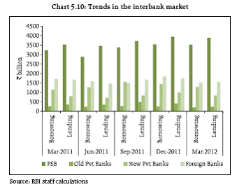
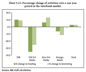
Network Analysis of the Financial System3 5.12 Network analysis of the financial system enables gauging the interconnectedness in the banking / financial system and assessing the risks arising out of possible contagion. It forms a critical part of the toolkit for macroprudential surveillance. 5.13 The size of the interbank market decreased marginally (2.8 per cent) between March 2011 and March 2012. The sharpest decline was evidenced in the case of the old private sector banks, which constitute 3 per cent of the entire market (Chart 5.10 and Chart 5.11).
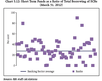
Trends in the short term borrowing of banks could engender liquidity risks… 5.14 An analysis of trends in the short term inter bank borrowing of banks indicated that such borrowings, which consists mostly of certificate of deposits (CDs), form a sizeable portion of the funds raised in the interbank market. The ratio of the banking sector’s short term interbank borrowings to total borrowings stands at around 27 per cent. Further, short term borrowings have grown by nearly 40 per cent over a period of one year, even as the overall quantum of inter bank borrowing has fallen. As short term borrowings typically engender rollover risks, trends in this regard will need to be monitored (Chart 5.12).
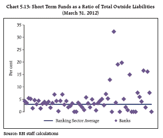
5.15 Short term inter bank borrowings as a proportion of total outside liabilities of banks (at about 3 per cent) was not, however, very significant. Nevertheless, there are some outlier banks which are heavily reliant on such borrowings and trends in this respect warrant greater attention (Chart 5.13).
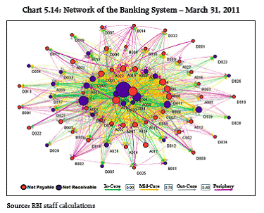
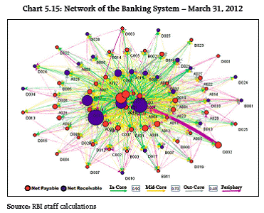
The banking system continues to remain interconnected 5.16 The country’s banking system displays a significant degree of interconnectedness. Together with this, a distinctly tiered structure of connectivity, where some banks are more connected than others, is also observed. An analysis of interconnectedness using the network model reveals that the level of connectivity in the system has increased slightly over the last year. (Box 5.1) Box 5.1: Network Statistics of the Banking System The network model uses various statistical measures to gauge the level of interconnectedness in the system. Some of the most important are as follows:
The trends in the aforesaid network statistics for the Indian banking sector indicate that the level of interconnectedness has remained broadly stable over the last five quarters though some statistics point to a marginal increase in connectivity.
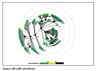
The systemic importance of some banks may have risen… 5.17 The majority of the banks appearing in the inner core of the network of the Indian banking system remained the same over the last one year.4 However, the number of net borrowers in the inner core has increased during this period, pointing to increased systemic importance of these banks. (Charts 5.14 and Chart 5.15)
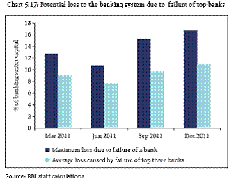
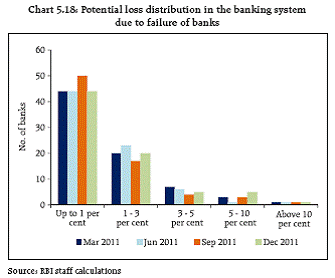
... as is also indicated by the results of contagion analysis 5.18 A contagion analysis using the network model reveals that the maximum possible loss to the banking system due to the failure of the ‘most connected’ bank has risen from 12 per cent of the capital of the banking system to over 16 per cent over the four quarters of 2011 (Chart 5.16). The average loss caused by the failure of the three ‘most connected’ banks has also increased (Chart 5.17). The contagion risks, however, appear to be confined to a few banks (Chart 5.18). Financial stability considerations, therefore, warrant that the risks posed by the increased interconnectedness of the few banks in the inner core need to be carefully monitored, through, inter alia, rigorous microprudential supervision of these entities.
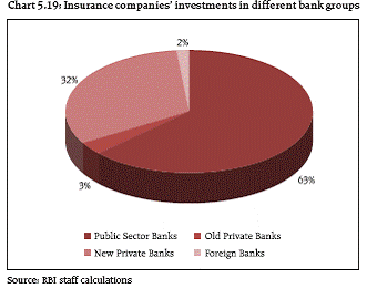
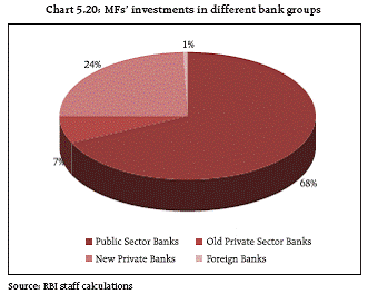
The major lenders in the financial system remain vulnerable to contagion risks 5.19 The network analysis of the broader financial system, presented in the previous FSR, had thrown up the interconnectedness among the banking, insurance and the mutual funds segments of the financial system. The analysis revealed that the largest net lenders in the system were the insurance companies and the Asset Management Companies (AMCs), while the banks were the largest borrowers. This renders the lenders vulnerable to the risk of contagion from the banking system. The random failure of a bank which has large borrowings from the insurance and mutual funds segments of the financial system may have significant implications for the entire system (Charts 5.19 and 5.20).
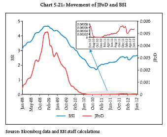
Banks reliant on the insurance sector and mutual funds, specially for short term funds… 5.20 SCBs were considerably dependent on borrowings from insurance companies and mutual funds. As at end-March 2012, nearly 27 per cent of the entire intra-financial system borrowings by banks was from insurance companies while another 37 per cent was from mutual funds. The reliance is particularly high in case of private sector banks (Table 5.3). Such borrowings from mutual funds and insurance companies constitute 6.8 per cent of the banking systems’ outside liabilities. 5.21 The bulk of the borrowing by SCBs from the mutual funds (81 per cent) consists of short term funds, which could engender rollover and liquidity risks. These borrowings almost entirely comprise CD issuances. In contrast, borrowings from insurance companies primarily have a longer maturity, with over 88 per cent of the borrowings carrying a remaining maturity of at least one year (Table 5.4). Banking Stability Measures and Estimation of Expected Shortfall 5.22 The stability of banking system was studied through various Banking Stability Measures, which gauge the impact of distress in one bank on the rest through direct and indirect links. For assessing these dependencies, the financial system is modeled as a portfolio of a specific group of banks (Segoviano and Goodhart, 2009). The model uses the Banking System’s Portfolio Multivariate Density (BSMD)6, which characterises both the individual and joint asset value movements of the portfolio of banks. The BSMD is recovered from the Probabilities of Distress (PoDs) of banks under analysis, which is observed empirically based on 99 per cent Value at Risk (VaR)7 of daily return on banks’ equity prices. Common distress in the system: JPoD and BSI 5.23 The probability of distress of the entire banking system, as measured by Joint Probability of Distress (JPoD), has been showing an upward trend over the last two years, though the probability continued to be low when compared to the level seen during the 2008-09.The Banking Stability Index (BSI), which measures the expected number of banks which could become distressed given that at least one bank becomes distressed, declined from the highs registered during 2008-09 till end-2010. Thereafter, it has been showing an increasing trend (Chart 5.21).
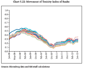
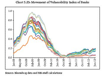
5.24 Trends in both JPoD and BSI indicate that interdependencies among banks have risen in recent times though they remain much below the level seen during the global financial crisis. Distress between specific banks: Toxicity & Vulnerability Index 5.25 The distress between specific banks has been measured based on Toxicity Index and Vulnerability Index8. As in the case of common distress indices, both the Toxicity and Vulnerability indices have shown a declining trend since the global financial crisis but the indices have been rising in recent periods, especially since 2011. (Charts 5.22 and 5.23).
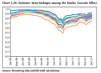
Cascade effects due to distress in a specific bank 5.26 Cascade effects are a measure of the probability of one or more banks becoming distressed, given that a specific bank becomes distressed. The measure reflects the systemic importance of a bank. Though these conditional probabilities do not imply causation; these can provide important insights into systemic interlinkages among the banks. The cascade probabilities show that the Indian banking system is highly interlinked and had a very high distress dependency during the financial crisis. This effect decreased in 2010, but has shown an increasing trend in recent periods (Chart 5.24).
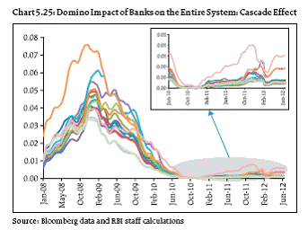
Domino Impact on the System: Cascade Effect 5.27 The systemic importance and ‘domino’ effect of a specific bank can be quantified as the likelihood of distress in the system dependent on distress in the bank (Chart 5.25). The domino impact for failure of the entire banking system has increased marginally in recent times.
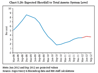
Expected Shortfall 5.28 The banking system’s Expected Shortfall (ES)9, which had a declining trend during 2008 to 2010, has been increasing since 2011. The ES was estimated to be around 8.5 per cent of total assets of the banking system in December 2008. Since then, the ES had declined significantly. However, beginning 2011, it has been showing an increasing trend, though the ES remains much below the levels observed during the global financial crisis. During March 2012, the ES stood at 3.4 per cent of total assets. Projected values of the ES for the coming quarters indicate that the shortfall may increase marginally (Chart 5.26).
Macro stress testing10 5.29 A series of macro stress tests was carried out to study the impact of various adverse macro shocks on banks’ credit quality. Four different econometric tools were used for the purpose. Apart from tests conducted at the system level, the exercise was also performed at bank-group and sectoral levels. In previous FSRs, the stress tests were conducted using various classical multivariate regressions. To ensure that the stress testing exercise takes cognisance of the tail events, quantile regression has also been adopted (Box 5.2). An assessment of systemic risk under different macroeconomic shocks from complementary angles was, thus, possible. Box 5.2: Macro Stress Test - Quantile Regression Approach The macro stress test is a tool to assess the vulnerability of the banking system to extreme but plausible adverse macroeconomic shocks. The stochastic relationship between banking stability, typically taken as a credit risk indicator defined by non-performing advances ratio or slippage ratio, and macro variables is established through statistical/econometric models. The results presented in previous FSRs were based on stress tests conducted using the techniques of multivariate logit regression, multivariate regression and multivariate panel regression. However, these classical regression analyses have their own limitations. First, they estimate the conditional mean of the dependent variable for the given set of independent variables (regressors) and, hence, this regression curve gives an incomplete picture. Second, these techniques assume that the impact of the independent variable on the dependent variable is symmetric and identical for different levels of the dependent variable, an assumption which may not hold under all circumstances. In particular, during a tail event, the relationship among the variables may change. To ensure that the stress testing exercise takes cognisance of the tail events, it is important that the exercise looks beyond the conditional mean and focuses on the tail. To this end, the technique of quantile regression tools, which enables explicit modeling of the tail of conditional distribution of the target variable, has been adopted. Quantile regression is one of the tools, which provides facility of modeling not only mean/median, but also explicitly models the tail of the conditional distribution by using other quantiles of the target variable.
Traditionally, quantiles are calculated by arranging the values of the variable in ascending order and then take the observation at which threshold is reached. Koenkar and Bassett(1978) introduced a completely new method to calculate quantile which is based on an objective function which is given as below, where, the concept of 'sorting' was replaced by the concept of 'optimising':
Whereas, the variance covariance matrix can be estimated by the three methods, namely, direct method, rank score method and resampling method. The quantile regression also captures the changing relative importance of macro variables along the conditional credit risk distribution at various quantiles. References IMF(2009), 'Global Financial Stability Report', April 2009. Koenker, R. and Bassett, G. (1978), 'Regression Quantiles' Econometrica 46 (1). Niel Schulze (2004), 'Applied Quantile Regression: Microeconomatric, Financial and Environmental Analyses', Inaugural-Dissertation, Tubingen. Schechtman Ricardo, Gaglianone W. P. (2011), 'Macro Stress Testing of Credit Risk Focused on the Tails', Working Paper Series 241, Banco Central Do Brasil. 5.30 The macro stress tests encompass a series of risk scenarios incorporating a baseline and two adverse macroeconomic scenarios representing medium and severe risk, where the shocks in the macroeconomic parameters are assumed to occur simultaneously (Table 5.5). The impact of the stress scenarios was assessed on the unconsolidated balance sheet of the domestic operations of SCBs. Essentially, the macro stress tests focus on different credit risk scenarios.
Credit quality may deteriorate under severe macro stress, but impact on CRAR is contained 5.31 The non performing asset (NPA) levels projected through different models suggest that, under the baseline scenario, NPAs are expected to be in the range of 3.3 to 3.5 per cent by March 2013. Under the stress scenarios, they could increase to 3.7 to 4.1 per cent (the medium risk scenario) and 4.1 to 4.6 per cent (the severe risk scenario). Under the severe risk scenario, the system level CRAR12 of commercial banks could decline to 12.5 per cent by March 2013, which still remains well above the regulatory requirements (Tables 5.6 and 5.7).
Impact of the risk scenarios varies across bank groups, but all groups are resilient 5.32 The impact of the risk scenarios varied across bank groups. The CRAR of public sector banks, under the severe stress scenario could fall to 11.5 per cent while the CRAR of the other bank groups is expected to be higher given the higher level of CRAR under the baseline scenario (Tables 5.8 and 5.9). The impact of risk scenarios vary across different sectors 5.33 The impact of the different risk scenarios on the level of NPAs in different sectors varied with the maximum impact evidenced in the Food Processing, Engineering and Iron and Steel sectors. The effect on NPAs in agriculture in this macro stress test analysis appears to be marginal (Table 5.10).
1The bars in Charts 5.1 and 5.2 represent the weighted aggregate of number of respondents who have identified the corresponding risk, the weights representing the probability assigned by the respondent to the occurrence of the risk. 2 The SLI uses the following four indicators representing various segments of the market: Weighted Average Call Rate - RBI Repo Rate; 3 month Commercial Paper (CP) Rate - 3 month Certificate of Deposits (CD) Rate; 3 month CD Rate - 3 month Forex Market Implied Deposit Rate; and Weighted Average Call Rate - 3 Month Overnight Indexed Swap (OIS) Rate. The index is based on 'standard normal' or 'variance-equal weighted' method and a value above zero would indicate above 'normal' levels of liquidity related stress in the system. 3 The network analysis has been conducted based on data in respect of bilateral fund based and non-fund based exposures between banks, asset management companies, insurance companies, NBFCs, financial institutions and urban cooperative banks. The transactions where the settlement takes place through a central counterparty have not been reckoned. The Network model used in the analysis has been developed by Professor Sheri Markose (University of Essex) and Dr. Simone Giansante (Bath University) in collaboration with the Financial Stability Unit, Reserve Bank of India. 4 A tiered structure is one where different institutions have different degrees or levels of connectivity with others in the network. In the present analysis, the most connected banks (based on their eigenvector centrality) are in the inner most core (at the centre of the network diagrams in Charts 5.14 and 5.15). Banks are then placed in the mid core, outer core and the periphery (the respective concentric circles around the centre in the diagrams), based on their level of relative connectivity. The range of connectivity of the banks is defined as a ratio of each bank’s in degree and out degree divided by that of the most connected bank. Banks that are ranked in the top 10 percentile of this ratio constitute the inner core. This is followed by a mid core of banks ranked between 90 and 70 percentile and a 3rd tier of banks ranked between 40 and 70 percentile. Banks with connectivity ratio of less than 40 per cent are categorised as the periphery. The colour coding of the links in the tiered network diagram represents the borrowing from different tiers in the network (for example, the green links represent borrowings from the banks in the inner core). 5 For a complete description of the methodology on the contagion analysis, please refer to FSR for December 2011 6 A complete description of the methodology was presented in the third issue of the Financial Stability Report, June 2011 7 The methodology for calculation of PoDs has been revised in this FSR as compared to the method used in FSR December 2011. The calculated PoDs are used as an input for derivation of JPoDs and the Banking Stability Measures as well as the Expected Shortfall. Earlier, threshold for calculation of PoDs were derived based on daily equity price returns since January 2007. Since during the financial crisis of 2008-09, the Indian banking equity prices recorded higher decline in return as compared to the current time as well as before the crisis, the threshold return limit (VaR) was set at a much lower level. Hence, the empirically observed PoDs were unable to capture the relative variation of equity return during the current period. Therefore, to overcome this limitation, the revised calculations of PoDs are based on the threshold derived after excluding the period of the financial crisis (i.e. on the daily equity price return since January 2010). All the measures show a slight upward movement (as compared to results published earlier). Further, to capture stress event in a broader way, the revised PoDs are based on 99 per cent VaR instead of 99.5 per cent VaR. 8 The Toxicity Index (TI) is the average probability that a bank under distress may cause distress to another bank in the system while the Vulnerability Index (VI) quantifies the vulnerability of a bank given distress in the other banks in the system.
10 The methodology is in the Annex. 11 The adverse scenarios were derived based on up to 1 standard deviation of 10 years historical data for medium risk and 1.25 to 2 standard deviation of 10 years historical data for severe risk. These stress scenarios are stringent and conservative assessments under hypothetical-severely adverse economic conditions and should not be interpreted as forecasts or expected outcomes. The projections are based on data pertaining to the fourth quarter of 2011-12. The macroeconomic shocks have been assumed to occur in the first quarter of 2012-13. |
|||||||||||||||||||||||||||||||||||||||||||||||||||||||||||||||||||||||||||||||||||||||||||||||||||||||||||||||||||||||||||||||||||||||||||||||||||||||||||||||||||||||||||||||||||||||||||||||||||||||||||||||||||||||||||||||||||||||||||||||||||||||||||||||||||||||||||||||||||||||||||||||||||||||||||||||||||||||||||||||||||||||||||||||||||||
Page Last Updated on:


