 IST,
IST,
Real Time Business Conditions Index: A Statistically Optimal Framework for India
Dipankar Biswas,* The measurement of business conditions on real time basis is a challenging task as the state of real economy is constantly evolving. In this context, in order to achieve an accurate and timely estimate of the state of real activity in a systematic, replicable and statistically optimal manner, this paper proposes a framework to construct a real-time business conditions index for India. The study is primarily motivated by the seminal work of Aruoba, Diebold and Scotti (2009), which proposed a high frequency business conditions assessment for the US economy. Based on various economic indicators measured at different frequencies, this paper develops a real-time business conditions index for India following a dynamic factor model framework for extracting signals from continuously evolving states. A Kalman filter routine is used for signal extraction from state-space representation as well as evaluation of likelihood function. Empirical results show that this coincident indicator tracks the overall economic activity reasonably well. JEL Classification : C61, E32, E37 Keywords : Business cycle; Dynamic factor model; Turning points; State-space model; Expansion Introduction The state of the real economy of a country evolves in a continuous fashion. Economic agents and policy makers, making decisions in real time, require accurate and timely estimates of the state of real activity. In the light of the changing nature of the economy, where more and more activities are being channelised through both organized and unorganized business sectors, the assessment of business conditions on real time basis is of paramount importance, particularly for central banks. From mid-1980s until 1998, the Reserve Bank of India (RBI) used a monetary-targeting framework. In the year 1998, the RBI’s Working Group on Money Supply, in its report, pointed out that monetary policy exclusively based on money demand could lack precision and hence it was necessary to monitor a set of additional indicators for monetary policy formulation. Accordingly, the RBI adopted a multiple indicator approach from 1998 wherein, besides monetary aggregates, information pertaining to currency, credit, fiscal position, merchandise trade, capital flows, inflation rate, exchange rate, refinancing and transactions in foreign exchange etc., were juxtaposed with data on output and the real sector activity for drawing policy perspectives. Monitoring a wide range of variables and studying their dynamic interactions are now possible partly because of the development of more sophisticated econometric models. In this context, in 2002, the RBI’s Working Group of Economic Indicators provided importance to deal with the business cycle analysis and to construct a composite index of leading indicators for Indian economy. In 2007, the RBI’s Working Group of Leading Indicators for Indian Economy, in its report, recommended two series, viz., monthly Index of Industrial Production (IIP) and quarterly Non-Agricultural GDP (NAGDP), as the reference frame of business cycle in India. The Group also constructed Composite Index of Leading Indicators (CILI) for each of these two reference series following international best practices. As proposed by the Group, the outlook for business cycle movement for 2-3 quarters ahead is regularly examined internally in RBI and serves as an important input to the monetary policy making. It has been, however, observed that the proposal of the Working Group of Leading Indicators to provide an outlook for business condition of the Indian economy is not sufficient on real time basis due to the following reasons. Firstly, most frequent data used for developing leading indicators is observed on monthly basis. For real time measurement, moving beyond the monthly frequency is a basic prerequisite. Some important indicators (e.g., asset prices, yield curve term premium) are observed at daily frequency, which potentially contain important information on the overall economic activity. Secondly, the report did not take into account the assumption of continuously evolving state of the economy, which is essential to real time measurement. Lastly, the provisional and partially revised data used for the leading index also affects the performance to predict future movements of aggregate economic activity in the real-time framework (Diebold and Rudebusch, 1991). Against this backdrop, we propose a framework motivated by the earlier work of Aruoba, Diebold and Scotti (2009), for the high frequency business conditions assessment for India in a systematic, replicable and statistically optimal manner. Giving the latest information of various macroeconomic indicators of different frequencies, our objective is to assess the current state of economic activity based on a real-time index and to update our assessment as more information flows in. Our assessment is as on today, and not beyond. In that sense, the index is coincident (not leading) to the business condition. The paper is organised as follows: Section II reviews select literature on the real-time data analysis. Section III describes the empirical analysis concerned with the development of real-time business conditions index for Indian economy. The description of software used for empirical analysis is mentioned in Section IV. Finally, Section V summarises the results, with a few concluding remarks in Section VI. In empirical econometrics, the use of real-time data is not a recent area of study. A long list of literature can be mentioned in this regard. Early studies of real-time data focused on the sensitivity of certain statistics to data vintage. Gartaganis and Goldberger (1955) did the first work on real-time data analysis. They mainly confined themselves to the properties of statistical discrepancy between Gross National Product (GNP) and gross national income in United States, after data were revised in 1954. Howrey (1978) focused on the use of preliminary data in econometric forecasting and indicated clearly that the intelligent use of preliminary data would be expected to result in a meaningful reduction in prediction error variances. Diebold and Rudebusch (1991) examined the ability of composite index of leading economic indicators to predict future movements in aggregate economic activities based on real-time analysis. They used the provisional and partially revised data for the leading index that were actually available historically, along with recursive out-of-sample forecasts. They found substantial deterioration of forecasting performance in the real-time framework. Orphanides and Simon van Norden (2002) examined the reliability of several detrending methods for estimating the output gap in real time. They focused on the extent to which output-gap estimates were updated over time as more information arrived and data were revised. They suggested that, great caution would be required for measuring output gap on real-time basis. Later research posed the problem more formally as a signalextraction problem. Evans (2005) focused on estimating high-frequency GDP, equated business conditions with GDP growth and used state space methods to estimate daily GDP growth using data on preliminary, advanced, and final releases of GDP and other macroeconomic variables. Anderson and Gascon (2009) used a state-space model to estimate the “true” unobserved measure of total output in the US economy. The analysis used the entire history (i.e., all vintages) of selected real-time data series to compute revisions and corresponding statistics for those series. The revision statistics, along with the most recent data vintage, were used in a state-space model to extract filtered estimates of the “true” series. In the Indian context, some studies (Dua and Banerji, 1999, 2004) related to business cycles and coincident economic indicators are important. These studies use the classical NBER approach to determine the timing of recessions and expansions in the Indian economy, as well as the chronology of growth rate cycles, viz., the timing of pickup and slowdown in economic growth. The reference chronology for business as well as growth rate cycles is determined on the basis of the consensus of key coincident indicators of monthly frequency along with a composite coincident index comprising those indicators, which track fluctuations in current economic activity. However, our aim is to assess the current state of economic activity based on the latest information of various macroeconomic indicators of varying frequencies. This study is primarily motivated by an empirical study of Aruoba, Diebold and Scotti (2009) on the US economy. They constructed a framework for measuring economic activity at high frequency, potentially in real time. They used a variety of stock and flow data observed at mixed frequencies and performed a prototype empirical application for illustrating the gains achieved by moving beyond the customary monthly data frequency. The four key ingredients of their work are as follows: 1. Treatment of business conditions as an unobserved variable, related to the observed indicators. Latency of business conditions is consistent with economic theory (e.g., Lucas 1977), which emphasizes that the business cycle is not about any single variable, but the dynamics and interactions (or co-movements) of many variables. 2. Explicit incorporation of business conditions indicators measured at different frequencies. Important business conditions indicators arrive at a variety of frequencies, including quarterly (e.g., GDP), monthly (e.g., industrial production), weekly (e.g., employment), and continuously (e.g., asset prices), and the incorporation of all of them provides continuously updated measurements. 3. Explicit incorporation of indicators measured at high frequencies. As the goal is to track the high frequency evolution of real activity, it is important to incorporate (or at least not exclude from the outset) the high frequency information flow associated with high frequency indicators. 4. Extraction and forecasting of latent business conditions using linear yet statistically optimal procedures, which involve no approximation. The appeal of exact as opposed to approximate procedures is obvious, but achieving exact optimality is not straight forward, due to complications arising from temporal aggregation of stocks versus flows in systems with mixed-frequency data. The study proposed a dynamic factor model that permitted optimal extraction of the latent state of macroeconomic activity being illustrated by a four-variable empirical application and in a parallel calibrated simulation (detailed theory is mentioned in the technical appendix). The following four indicators with varying frequencies were chosen as business conditions indicators: 1. Yield curve term premium, defined as the difference between 10-years and 3-months US Treasury yield, at daily frequency. 2. Initial claims for unemployment insurance, a weekly flow variable. 3. Employees on non-agricultural payrolls, a monthly stock variable. 4. Real GDP, a quarterly flow variable. The real activity indicator thus obtained from the empirical analysis threw new light on the area of business cycle measurement and simultaneously outperformed the so-called National Bureau of Economic Research (NBER) chronology in some economic as well as statistical sense. First, although the real activity indicator broadly coincided with the NBER chronology, it had a propensity to indicate earlier turning points, especially peaks. Second, the indicator was available at high frequency and hence, a useful “nowcast”, whereas the NBER chronology was available only monthly and with very long lags. Third, it was evident that incorporation of weekly data in real activity indicator was very helpful for providing real time information, as compared to NBER chronology. However, incorporation of daily data did not improve the performance of the indicator; still a daily state space setup was needed to accommodate the variation in weeks per month and weeks per quarter. Fourth, based on a simulation calibrated to the empirical results, it was observed that, incorporating high frequency data improved the accuracy of the extracted factor. Lastly, the real time performance (preferably, daily) of the business conditions would be assessed at any point of time by re-estimating the system based on latest-vintage data. Presently, six macroeconomic indicators are used to construct the Aruoba-Diebold-Scotti Business Conditions Index (ADS Index). These are weekly initial jobless claims, quarterly real GDP, monthly payroll employment, monthly industrial production, monthly real personal income less transfers, and monthly real manufacturing and trade sales. All these are important and widely monitored. The ADS Index is updated weekly, following the release of that week’s new and/or revised component indicator data. Section III It has been pointed out in Section 2 that, the business conditions of an economy are latent, and are related to some observed indicators. In order to develop a real time business conditions indicator in Indian context, the prime objective is to select those observed indicators from the existing information base on the same lines as was mentioned in the study of Aruoba, Diebold and Scotti (2009). The information base includes national income aggregates, index of industrial production, capital market performance, monetary and banking statistics, price statistics, fiscal statistics, trade data, etc. Some important series along with their source, frequency, availability, and economic as well as statistical justification for inclusion in the selected list are discussed in Table 1.
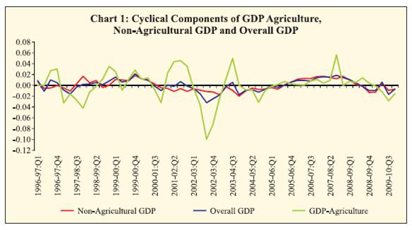
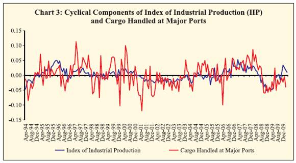
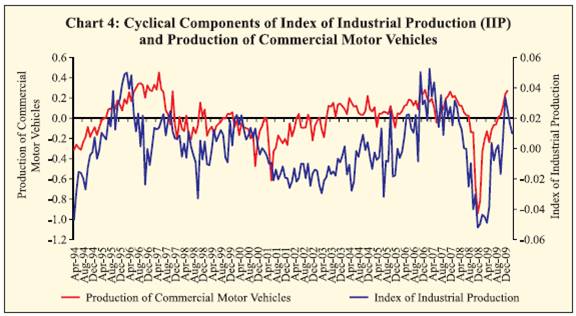
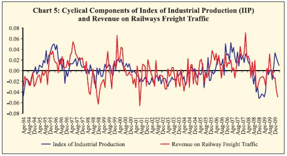
a. Real Gross Domestic Product - Ideally the Real Gross Domestic Product (GDP) represents almost all aspects of the economic activities. In the literature of business cycle, the cyclical fluctuation of Real GDP is a well-accepted reference frame of the business conditions of the economy as it includes all the three sectors viz., primary, secondary and tertiary. In India, the Central Statistics Office (CSO) of Ministry of Statistics and Programme Implementation releases the quarterly figures of GDP with a two month time lag. In the report of RBI’s Working Group of Leading Indicators for Indian Economy, the quarterly Non-agricultural GDP (NAGDP) was taken as a reference series of business cycle due to the dependence of agricultural sector on monsoon performance. In the context of the Indian economy, the agriculture and allied sector contributes almost 20 per cent to the total GDP. However, the performance of agriculture sector depends heavily on rainfall. The high volatility in agricultural sector may be observed from the movement of cyclical component of GDP Agriculture with standard deviation 0.26 (Chart 1). On the other hand, the standard deviation of each of the Overall GDP and Non- Agricultural GDP cycles is 0.13. Moreover, Chart 1 depicts similar movements of Overall GDP and Non-Agricultural GDP cycles (with correlation 0.87). Based on these observations, Nonagricultural GDP is considered more preferable than overall GDP. b. Index of Industrial Production – In the ADS index, out of six macroeconomic series, one is monthly industrial production and accordingly, in this study, monthly Index of industrial Production (IIP) has also been considered. The index is regularly published by CSO with a two month lag. It may also be mentioned that, OECD uses monthly Industrial Production as the reference series for business cycle analysis. Chart 2 presents the coincidental movements of Non-Agricultural GDP and IIP cycles with correlation 0.81. As the Non-Agricultural GDP has nearly 83 per cent share in overall GDP, it is well justified that IIP also reflects the business conditions of the economy with frequency higher than quarterly intervals. c. Indicators observing industrial activities – There are some other indicators that show the performance of industrial activities. Transportation of goods by road is a good indicator of industrial production process. Thus ‘Production of commercial motor vehicles’ is taken as an indicator. Moreover, increased levels of production, consumption and trade also get reflected, particularly in a large country such as India, in increased transportation of goods. Thus, the two series, viz., ‘Cargo Handled at Major Ports’ and ‘Revenue on Railways Freight Traffic’ are also considered in this study. The data of these series are regularly released in the monthly capsule report of CSO with two months lag. The movements of cyclical components of the three industrial activities indicators vis-à-vis IIP are presented in Charts 3 to 5. All show coincidental movement with IIP cycle.
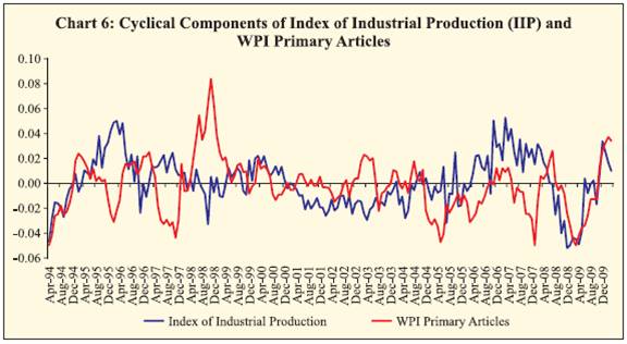
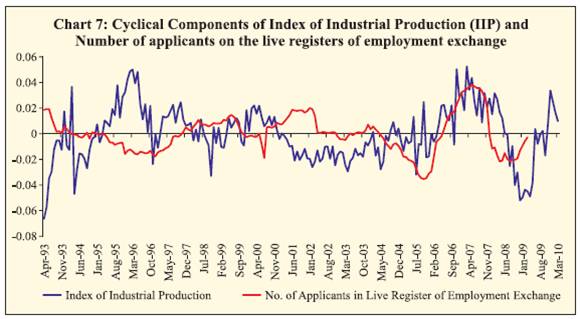
d. WPI Primary Articles – In the ADS Index, the price factor was not considered directly, but the daily yield curve term premium (i.e., difference between 10-year and 3-months US Treasury yield) had taken into account inflation expectations to some extent. In our study, we consider WPI Primary Articles compiled by Ministry of Commerce and Industries, due to the following reasons. (i) WPI Primary Articles data are available at weekly frequency1. Although WPI Manufactured Products is more related to industrial production than WPI Primary Articles, it is presently compiled on monthly basis. Moreover, although WPI of ‘Fuel and Power’ is available on weekly basis, the prices of some products included in the ‘Fuel and Power’ group are administered by the government. (ii) The cyclical movement of WPI Primary Articles is somehow coincident to IIP cycle, although divergence is clearly observed in most cases (Chart 6). e. Employment and Unemployment indicator – The comprehensive employment series, which is available on a regular basis, is the estimated average daily employment in factories. But it is available only on an annual basis. Data on unemployment rate are not complied on a regular basis. The series, ‘Number of applicants on the live registers of employment exchange’, released in Monthly Abstract of Statistics by CSO, gives some indication of the number of unemployed in the cities. But this suffers from the well-known limitations such as the changing (increasing) number of unemployment exchanges over the years, possibility of incomplete as well as multiple registrations, registration by those currently employed because they are looking for better jobs or through failure to cancel registration, etc. Despite these limitations, Chitre (2001) found this series as a useful coincident indicator of the industrial production and, therefore, is included in the present study (Chart 7). Another limitation of the series is its long lag period for releasing the data. For example, the Monthly Abstract of Statistics, September-October 2009 publication released the data upto March 2009. f. Yield Curve Term Premium – In the study of Aruoba, Diebold and Scotti (2009), the only series with daily frequency was yield curve term premium, defined as the difference between 10-years and 3-months US Treasury yield. On the same lines, in this study, the difference between yields of 10-years government securities and 91-days Treasury Bills is included in the list. These data are available on real-time basis. g. BSE Sensex – Another daily indicator, as mentioned by Aruoba, Diebold and Scotti (2009), is asset price. As a proxy of asset price, daily Sensex data of Bombay Stock Exchange (BSE) has been examined. It was observed that, in connection with the economic activity of the country, Sensex seems to be noisy as well as volatile. Also, on examining the cross correlation of BSE Sensex with Non- Agricultural GDP (NAGDP), IIP and weekly Foreign Exchange Reserve, we have seen that the correlation is not encouraging. h. Foreign Exchange Reserves - As selected indicators are expected to be highly correlated with each other, we have examined the cross-correlation among different series at different frequencies. It was found that, the Foreign Exchange Reserves, which was considered as a stock variable available at weekly frequency, has a poor correlation with the economic activity, i.e., NAGDP as well as with IIP, and hence is not considered fit for the requirement.
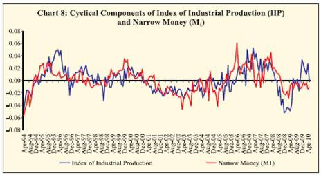
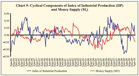
i. Money Supply and Narrow Money–Besides weekly variables, Narrow Money (M1) and Money Supply (M3) have been considered as fortnightly stock variable for testing coincidence with IIP and NAGDP cyclical components. The cross-correlations of M1 and M3 with NAGDP and IIP separately were examined and found that Narrow Money had a better relationship with IIP and GDP than Money Supply and hence was selected (Table 5 and Charts 8 and 9).
Based on the above-mentioned indicators as well as the methodology (described in the Technical Appendix), four indicators were finally selected (Table 6). We implimented this methodology using a program in RATS software to construct a real-time business conditions index in the Indian context. Instead of weekly variable (as used in ADS index), we have considered here a fortnightly available stock variable, i.e. Narrow Money (M1).
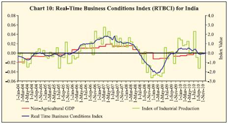
First, we have extracted the cyclical component from the four selected series as we try to find an indicator for business cycle. We did the extraction based on the following procedure: I. Seasonal adjustment of the series using X-12 ARIMA methodology. II. HP Filter to remove the smoothed trend from the seasonally adjusted series and finally extracting the cyclical component. Then the series having cyclical component only has been used in the program as an input. After that, we have defined the matrices of the state-space model following the theory stated in the paper by Aruoba, Diebold and Scotti (2009). In their paper, they considered a weekly flow variable, but in our case we have considered a fortnightly stock variable. Again, instead of monthly stock variable, we have considered a flow variable. The matrix coefficients have been changed accordingly. We have used Dynamic Linear Model for estimating the coefficients. We obtain our start-up values in two steps as follows. In the first step, we use only daily and stock variables, which drastically reduce the dimension of the state vector, resulting in very fast estimation. This yields preliminary estimates of all measurement equation parameters for the daily and stock variables and all transition equation parameters, as well as a preliminary extraction of the factor (via a pass of the Kalman smoother). In the second step, we use the results of the first step to obtain startup values for the remaining parameters, that is, those in the flow variable measurement equations. We simply regress the flow variables on the smoothed state extracted in the first step and take the coefficients as our start-up values. With the model cast in state-space form, and for given parameters, we use the Kalman filter and smoother to obtain optimal extractions of the latent state of real activity. Based on the four finally selected indicators, viz., daily Yield curve term premium, fortnightly Narrow Money (M1), monthly Index of Industrial Production (IIP), and quarterly Non-Agricultural GDP (NAGDP), the Real-time Business Conditions Index (RTBCI) was constructed (Chart 10). Data period of the selected variables is presented in Table 7. Chart 10 displays the cyclical movements of Non-Agricultural GDP (NAGDP) and Index of Industrial Production (IIP) along with the daily movement of RTBCI. It is observed that there is a coincidental movement among these three series. The movement of RTBCI beyond the vertical red line indicates the state of the economy which is otherwise not observed from the macro aggregates. The momentum as per the RTBCI as on December 10, 2010, indicates somewhat low acceleration of economic activity.
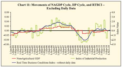
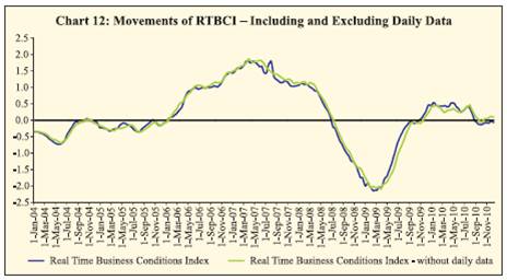
In order to see the importance of daily data for real-time measurement, a separate analysis was done to construct an index using the three selected indicators except daily “Yield curve term premium” data. The reason behind this is to examine if the RTBCI using fortnightly data performs better than the earlier index constructed using daily data. Chart 11 displays the cyclical movements of Non-Agricultural GDP (NAGDP) and Index of Industrial Production (IIP), along with the daily movement of RTBCI without daily data. Although this chart indicates co-movement between these three series, the next step is to search for any lag difference between the movements of RTBCI and RTBCI without daily data. Chart 12 displays the movements of RTBCI and RTBCI without daily data. In this chart it is observed that, the turning points of RTBCI including daily data is earlier than those of RTBCI without daily data. The lag difference varies approximately from 1 to 6 weeks. This implies that, if the turning point occurs in the business cycle movement, then RTBCI will capture the turning point earlier than RTBCI without daily data. For example, the turning point occurred in January 2009 in IIP cycle was captured by RTBCI (value corresponding to January 3, 2009 was the lowest) four weeks earlier than that captured by RTBCI without daily data (value corresponding to January 31, 2009 was the lowest). This justifies the importance of usage of daily data while constructing the Index. Real time decision making requires accurate and timely understanding of the state of real activity. In the light of the changing nature of the economy where increasingly more and more activities are channelised through both the organized and unorganized business sectors, the measurement of business condition on real time basis is extremely difficult. In this context, in order to achieve an accurate and timely estimate of the state of real activity in a systematic, replicable and statistically optimal manner, this paper proposes a framework to construct a real-time business conditions index for India. Based on various economic indicators measured at different frequencies, this paper develops a real-time business conditions index for India following a dynamic factor model framework for extracting signals from continuously evolving states. A Kalman filter routine is used for signal extraction from state-space representation as well as evaluation of likelihood function. Empirical results show that this coincident indicator tracks the overall economic activity reasonably well. Technical Appendix As indicated earlier, the framework for measuring real time economic activity at high frequency as presented in this paper was developed by Aruoba, et al. (2008). Detailed methodology is documented there. A brief description is presented in this technical appendix.The frequency of the dynamic factor model considered here is daily. However, daily data are mostly not observed for major variables and so will be shown missing. As a result, missing data and temporal aggregation were treated explicitly. In this process, measurement equations were obtained for both stock and flow variables which were observed. This allowed us to incorporate lagged state variables in the measurement equations and also the trend, which are important characteristics of macro data. a. Dynamic Factor Model: Framework for Daily Frequency Though this approach can handle higher (intraday) frequencies, we
have assumed that the state of the economy evolves at daily frequency.
Obviously, there will be many macro variables which are observed at
monthly or quarterly or annual frequency and hence are not observed
daily. If the underlying business conditions 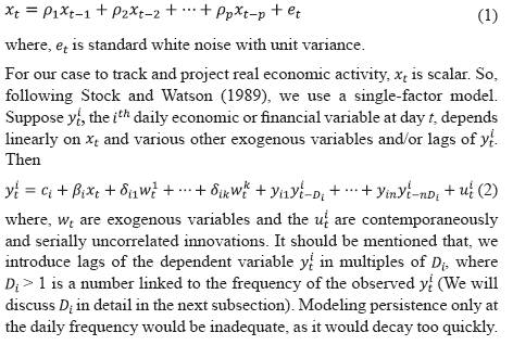 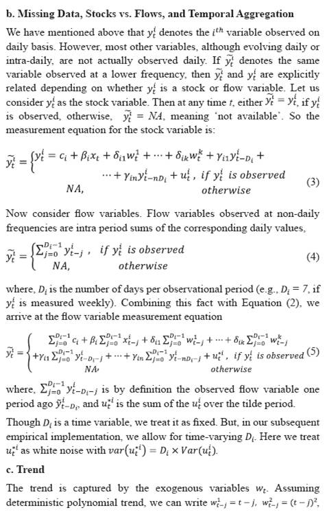 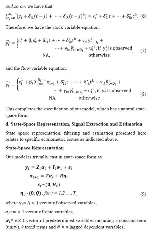 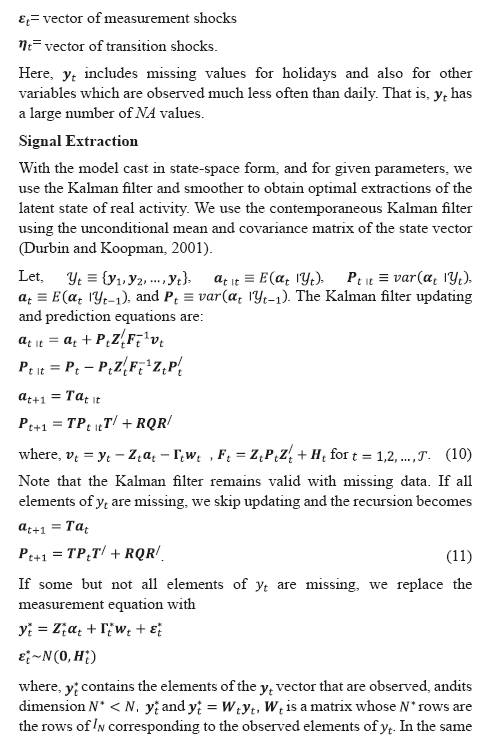  e. Empirical Application We now present a simple application involving the daily term premium, fortnightly Narrow Money, monthly IIP, and quarterly NAGDP. We describe in turn the data, the specific variant of the model that we implement subtleties of our estimation procedure, and our empirical results. Business Conditions Indicators Our analysis covers the period from December 1, 2003 through July 2, 2010, which are 2406 observations of daily data. We use a seven-day week and four indicators. Moving from highest frequency to lowest frequency, the first indicator is the yield curve term premium, defined as the difference between 10-year Government securities and 3-month Indian Treasury yields. We measure the term premium daily; hence there are no aggregation issues. We treat holidays and weekends as missing. The second indicator is Narrow Money, a fortnightly stock variable covering the seven-day period from Sunday to Saturday. We set the end-of-fortnight value to the end-of-fortnight daily value, and we treat other days as missing. The third indicator is IIP, a monthly flow variable. We set the end-of-month value to the sum of the daily values within that month, and we treat other days as missing. The fourth and final indicator is NAGDP, a quarterly flow variable. We set the end-ofquarter value to the sum of daily values within the quarter, and we treat other days as missing. Basically, we want the variables chosen to illustrate the flexibility of our framework. Hence we choose four variables measured at four different frequencies ranging from very high (daily) to very low (quarterly), and representing both stocks (term premium, narrow money) and flows (IIP, NAGDP). Since we are seeking a ‘Business Cycle’ indicator, we have extracted the cyclical component from the data (except the daily variable). This cyclical series is taken as our input. Model Implementation In the development thus far we have allowed for general polynomial trend and general AR(p) dynamics. In the prototype model that we now take to the data, we make two simplifying assumptions that reduce the number of parameters to be estimated by numerical likelihood optimization. First, we de-trend prior to fitting the model rather than estimating trend parameters simultaneously with the others, and second, we use simple first-order dynamics throughout. In future work, we look forward to incorporating more flexible dynamics but, as we show below, the framework appears quite encouraging even with simple AR(1) dynamics. 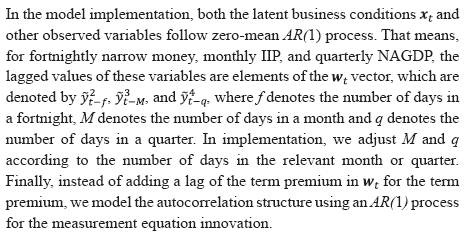 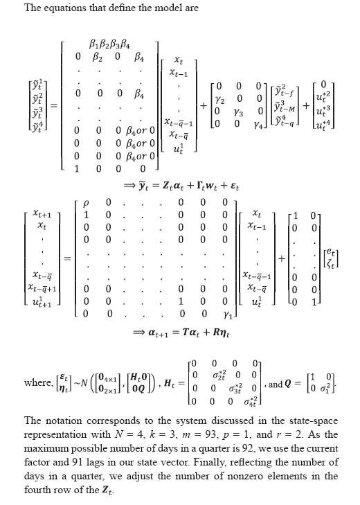 References Anderson, Richard G. and Gascon Charles S., (2009), “Estimating U.S. Output Growth with Vintage Data in a State-Space Framework”, Federal Reserve Bank of St. Louis Review, July/August, 91(4), pp. 349-69. Aruoba, S. B. (2008), “Data Revisions Are Not Well-Behaved,” Journal of Money, Credit and Banking, 40, 319–340. Aruoba, S. B., Diebold Francis X. and Scotti Chiara, (2009), “Real- Time Measurement of Business Conditions”, Journal of Business and Economic Statistics, October, Vol. 27, No. 4, pp. 417-427. Burns, A. F., and Mitchell, W. C., (1946), Measuring Business Cycles, New York: NBER. Diebold, Francis X. and Rudebusch, Glenn D., (1991), “Forecasting Output with the Composite Leading Index: A Real-Time Analysis”, Journal of the American Statistical Association, September, 86(415), pp. 603-10. ----------------, (1996), “Measuring Business Cycles: A Modern Perspective,” The Review of Economics and Statistics, 78, 67–77. Diebold, F. X., Rudebusch, G. D., and Aruoba, S. B., (2006), “The Macroeconomy and the Yield Curve: A Dynamic Latent Factor Approach,” Journal of Econometrics, 131, 309–338. Dua, P., and Banerji, A., (1999), “An Index of Coincident Economic Indicators for the Indian Economy”, Journal of Quantitative Economics, 15, 177-201. ----------------, (2004), “Coincident Index, Business Cycles and Growth Rate Cycles: The Case of India” in Macroeconomic Modelling, ed., K. Krishnamurty and V. Pandit, Oxford University Press. Durbin, J., and Koopman, S. J., (2001), Time Series Analysis by State Space Methods, Oxford University Press. Evans, M. D. D., (2005), “Where Are We Now?: Real Time Estimates of the Macro Economy,” The International Journal of Central Banking, September,127–175. Gartaganis, Arthur J. and Goldberger, Arthur S., (1955), “A Note on the Statistical Discrepancy in the National Accounts”, Econometrica, April, Vol. 23, No. 2, pp. 166-173. Hamilton, J. D., (1989), “A New Approach to the Economic Analysis of Nonstationary Time Series and the Business Cycle,” Econometrica, 57, 357–384. Harvey, A.C., (1989), Forecasting, Structural Time Series Models and the Kalman Filter, Cambridge University Press. Howrey, E. P., (1978), “The Use of Preliminary Data in Econometric Forecasting”, The Review of Economics and Statistics, April, Vol. 60, No. 2, pp.193-200. ----------------, (1984), “Data Revision, Reconstruction, and Prediction: An Application to Inventory Investment,” Review of Economics and Statistics, 66,386–393. Liu, H., and Hall, S. G., (2001), “Creating High-Frequency National Accounts with State-Space Modelling: A Monte Carlo Experiment,” Journal of Forecasting, 20, 441–449. Mariano, R. S., and Murasawa, Y., (2003), “A New Coincident Index of Business Cycles Based on Monthly and Quarterly Series,” Journal of Applied Econometrics, 18, 427–443. Orphanides, A. and Norden, Simon van, (2002), “The Unreliability of Output-Gap Estimates in Real Time”, The Review of Economics and Statistics, November, Vol. 84, No. 4, pp. 569-583. Reserve Bank of India, (1998), “Report of the Working Group on Money Supply”, Reserve Bank of India, Mumbai. ----------------, (2002), “Report of the Working Group of Economic Indicators”, Reserve Bank of India, Mumbai. ----------------, (2007), “Report of the Technical Advisory Group on Development of Leading Indicators for the Indian Economy”, Reserve Bank of India, Mumbai. Stock, J. H., and Watson, M.W., (2002), “Macroeconomic Forecasting Using Diffusion Indexes,” Journal of Business & Economic Statistics, 20, 147–162. * The authors are working in the Department of Statistics and Information Management, Reserve Bank of India, Mumbai. Views expressed in the paper are those of the authors and not of the Reserve Bank of India. An earlier version of this paper was published as RBI Working Paper, WPS (DEPR): 3/2011. The authors are grateful to Prof. S. Boragan Aruoba, University of Maryland, US for helping to implement the methodology in the Indian context. 1 This was the case until January 14, 2012. Subsequently WPI headline and all its subcomponents are compiled on monhly frequency from February 2012. |
||||||||||||||||||||||||||||||||||||||||||||||||||||||||||||||||||||||||||||||||||||||||||||||||||||||||||||||||||||||||||||||||||||||||||||||||||||||||||||||||||||||||||||||||||||||||||||||||||||||||||||||||||||||||||||||||||||||||||||||||||||||||||||||||||||||||||||||||||||||||||||||||||||||||||||||||||||||||||||||||||||||||||||||||||||||||||||||||||||||||||||||||||||||||||||||||||||||||||||||||||||||||||||||||||||||||||||||||||||||||||||||||||||||||||||||||||||||||||||||||||||||||||||||||||||||||||||||||||||||||||||||||||||||||||||||||||||||
Page Last Updated on: September 12, 2023


