 IST,
IST,
Chapter V : Systemic Risk Assessment
The need for assessing build up of systemic risks has emerged, in the post crisis world, as a critical part of any framework for macroprudential surveillance. Central banks around the world are engaged in developing tools and techniques to accurately assess such risks to the financial system. In India too, upgrading technologies and adding to its existing toolkit for identifying and measuring systemic risks is a continuing endeavour. Simultaneously, there is a realisation that systemic risks are complex and measuring them with precision may be challenging - exercise of judgement is hence critical A Systemic Risk Survey has been instituted by the Reserve Bank to get the views of market participants and stakeholders to supplement its own assessment and that of the financial sector regulators and policy makers (as represented in the Sub Committee of the FSDC). A series of stability indices and maps (as presented in various Chapters of this Report) have been devised to assess movements in the various risk dimensions which have a bearing on the macro economy, the financial markets, the fiscal segment, the banking sector and the entire financial system. A Systemic liquidity Indicator attempts to measure the build up of stress scenarios in the availability of various types of liquidity in the system. A network model of inter-bank and intra financial sector exposures attempts to analyse contagion risks arising from an initially idiosyncratic problem that becomes more widespread in the cross section of the banking sector and the financial sector. Banking stability measures attempt to model the distress dependencies in the banking sector, among specific groups of banks and that associated with an individual bank. Finally, a series of macrofinancial stress tests focus on the impact of macro economic shocks on the financial system. 5.1 The recent financial crisis presented a stark example of the consequences of build up of systemic risks. It demonstrated that if systemic risks have gradually accumulated up to a point, then even a relatively small shock can amplify and lead to widespread consequences for the stability of the financial system. 5.2 Post crisis, there emerged a clear consensus that in order to avoid such episodes of financial instability, financial authorities need to better identify, assess and manage the systemic risks prevailing in the financial sector. Simultaneously, there emerged a realisation that identification of systemic risks is a task which is far from straightforward given that systemic risks per se are complex and multifaceted. There was also increasing realisation that in order to see "both the forest and trees"1 effectively, there is a need to have a wide range of measures and tools covering different aspects of systemic risks. 5.3 A host of new quantification measures have, post crisis, emerged in academic literature, while central banks, in their quest for maintaining financial stability, are developing tools and techniques which will help identify and measure systemic risks. The broad objective is to support macro-prudential surveillance of the financial system. 5.4 With the establishment of the Financial Stability Unit in the Reserve Bank in 2009 with a mandate for, inter alia, "conduct of macro-prudential surveillance of the financial system on an ongoing basis", a series of systemic risk assessment measures and projects are being undertaken. The objective is to develop tools and methodologies which could be used to identify, assess and monitor potential threats to the stability of the domestic financial system. 5.5 The efforts at systemic risk assessment are aimed at capturing various dimensions of systemic risks through different models. A series of stability indicators/ maps attempt to capture the different risks dimensions which affect the stability of different segments of the economy [the macro economy, financial markets, the fiscal, the banking sector] as well as the entire financial system. Movements in these dimensions are then used to assess whether or not risks to stability are emerging. The signals thrown up by these indicators/maps have been presented in the appropriate Chapters of this Report. The different Sections of this Chapter present the results of broad based attempts to assess and capture the movements of systemic risks per se. The analytical assessment of the indications for the emergence of such risks based on a series of initiatives/models adopted by the Reserve Bank add to the overall assessment of risks to financial stability in this issue of the Financial Stability Report. Systemic Risk Survey Systemic Risk Survey as an additional tool to assess build-up of risks... 5.6 The Reserve Bank instituted, in October- November 2011, its first Systemic Risk Survey with a view to gauge perceptions of market participants and other stakeholders about the key sources of risk to the Indian financial system. The Survey will be a biannual exercise. The endeavour is expected to complement Reserve Bank's own assessment of risks to financial stability. The Survey captured the views of a wide range of market participants and stakeholders... 5.7 The Survey respondents included a group of about 100 select individuals from banks, financial institutions, insurance companies, asset management companies, non-banking financial companies, primary dealers and broking firms. The respondents also included representatives from industry associations, rating agencies, clearing corporations as well as select academicians and thinkers. ...both on specific risks and the degree of confidence in the stability of the system 5.8 The Survey attempts to capture the views of market participants and other stakeholders on the specific systemic risks facing the financial system, as also their assessment of the probability of high impact events affecting the global financial system and the Indian financial system, both in the short and the medium run. A separate set of questions elicited the respondents' degree of confidence in the stability of the global and domestic financial system and also how it has changed due to the events unfolding over the last six months. Asset quality - the risk with the highest probability of occurrence 5.9 The majority of the respondents identified deterioration in the asset quality of banks as the most significant risk to the financial system followed by risks from heightened market volatility, including exchange rate volatility, global risks, risks from high inflation and high interest rates. Other risks identified included fiscal risks, risks from excessive or slow regulatory responses and corporate risks including risks of corporate governance. There was the odd mention of risks from slow credit offtake, rating downgrade of the country and of domestic banks, terrorism, asset price bubbles, technology risk like cyber crime, failure of payments infrastructure, risks from the prevailing political situation, etc (Chart 5.1).
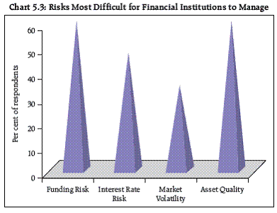
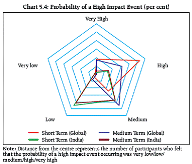
Risks from high inflation most difficult for the country to manage 5.10 The Survey respondents assessed that the risks from high inflation will be most difficult for the country to manage. The impact of global risks and increased market volatility would also be difficult for the system to manage as would risks from deterioration in asset quality (Chart 5.2). Participants from financial institutions felt that funding risks, risks from deterioration in asset quality, interest rates and from increased market volatility would be most difficult for their respective institutions to manage (Chart 5.3). Probability of a high impact event occurring in the global financial system high... could impact the domestic financial system 5.11 Over half the Survey respondents felt that the probability of a high impact event occurring in the global financial system was "High" in the short term, but were relatively more sanguine about the Indian financial system. In the medium term, the probability of a high impact event occurring in the global financial system was also high, though not as high as the short term (Chart 5.4). The probability of a similar event occurring in the domestic financial system was assessed to be lower. However, the majority of the respondents felt that the global developments would affect the Indian financial system, with over 40 per cent expecting the impact to be significant (Table 5.1). 5.12 The survey also reveals that the market confidence in the stability of the Indian financial system is significantly higher as compared to stability of the global financial system. Over 50 per cent of the respondents had little or no confidence in the stability of the global financial system, whereas more than 90 per cent of the respondents were 'very' or 'fairly' confident of the stability of the Indian financial system. The confidence of the respondents in the stability of the global financial system has largely decreased over the previous six months whereas it has remained substantively unchanged as far as the Indian financial system is concerned (Chart 5.5 and Table 5.2).
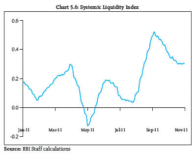
The Survey added to and mirrored the Reserve Bank's assessment of systemic risks 5.13 Overall, the findings of the Risk Survey mirrored the Reserve Bank's own assessment of systemic risks as outlined in the various chapters of this Report. The findings also attested to the confidence in the stability of the domestic financial system, though the degree of confidence in the global financial system was low and deteriorating. Systemic Liquidity Index (SLI)3 for India Liquidity has many forms 5.14 Liquidity is commonly understood as being of two types: funding and market liquidity. Funding liquidity refers to the ability of institutions to raise money from banks or in term money/ commercial paper markets or by repo-ing out existing securities to meet a cash outflow. Market liquidity refers to the ability to sell assets to raise cash with low impact costs. When firms sell assets, their balance sheet leverage does not increase whereas raising liquidity in money markets involves increasing their balance sheet size. The distinction between the two is important from the financial stability perspective. During the financial crisis, counterparty credit concerns led firms to rely on sale of assets (shrinking of balance sheets) since term money markets had frozen. Deleveraging eventually caused the turmoil in financial markets to spread to the broader economy in US and Europe causing a global recession. 5.15 Systemic liquidity for the purpose of the index is defined as the funding liquidity scenario in the banking sector, non-banking financial sector, the corporate sector and prevailing foreign currency liquidity. Current needs for liquidity are also influenced by expectations about availability of funds and their rates in future. So the index also uses a forward looking parameter. Multiple indicators for measuring liquidity are preferred 5.16 In order to measure liquidity, it is preferable to go in for a multiple indicator approach, which would be able to better capture the liquidity from a variety of dimensions. A SLI that measures liquidity conditions in the market has several uses. Firstly, it measures the level of liquidity and gives a quantitative assessment of its current level. Secondly, the time series of the index enables us to compare the improvement or otherwise in liquidity conditions vis-a-vis past levels. 5.17 The SLI uses the following four indicators representing various segments of the market. 1. Weighted Average Call Rate - RBI Repo Rate The weighted average call rate adjusted for the RBI repo rate captures information about the levels of funding stress in the banking system. The weighted average call rate has been adjusted to neutralise the impact of changes in the Reserve Bank's policy or repo rate on it as a rise in the latter does not automatically imply tougher liquidity conditions. 2. 3 month Commercial Paper (CP) Rate - 3 month Certificate of Deposits (CD) Rate Liquidity conditions for the commercial sector could be affected through amount, cost and maturity of credit that is extended. The SLI uses CP rates as an indicator of cost of funds for the commercial sector. This is important as stress in banking as well as non-banking sector's funding markets is sought to be covered under the SLI. The CP rate is reduced by the cost of banks' funds to extract the additional rise in cost for the commercial sector. 3. 3 month CD Rate - 3 month Implied Deposit Rate The SLI also uses the difference between 3 month CD Rate and 3 months Forward Implied Deposit Rate as an indicator. The reason for using this indicator is to increase the coverage of funding markets. Banks often use FX swaps to raise Rupee funds. The ones that do not maintain large buffers over and above the SLR of 24 per cent find this source of funding convenient. The FX swap frees them from the need of holding the less liquid SLR securities. The difference between domestic deposit and foreign exchange market implied deposit rates is a sign of stress in foreign exchange market based funding liquidity. 4. Weighted Average Call Rate - 3 Month Overnight Indexed Swap (OIS) Rate The SLI uses a forward looking indicator like 3 month OIS rate which points to market expectation about the future course of the overnight rate. For instance, the OIS market might be pricing a policy rate hike near term but several cuts subsequently. Interbank borrowing and lending has to take into account such expectations about future course of policy rates. At times of liquidity stress, the overnight rates go up but expectations about the longer term do not change if the factors driving the overnight rates are believed to be temporary. The flattening or steepening of the OIS yield curve gives clear signals about liquidity conditions and the perceptions about whether they are temporary or not. 5.18 The index has been constructed after experimenting with four different methodologies4 and the 'standard normal' or 'variance-equal weighted' method has been accepted as most appropriate. A value above zero would indicate above normal levels of stress in liquidity. Liquidity tightness remains elevated but acceptable 5.19 The liquidity deficit, which witnessed some stress in June 2011 due to quarterly advance tax payouts, eased in early July 2011, reflecting the drawdown of Central Government cash balances and transition to Ways and Means Advances (WMA)/Over Draft (OD). Average Liquidity Adjustment Facility (LAF) injections, which were around `49,000 crore in the first quarter of 2011- 12, dropped marginally to around `47,000 crore in the second quarter of 2011-12. After a gap of nearly five months, the LAF window went in to absorption mode in the beginning of October 2011. However, the liquidity conditions tightened again from October 7, 2011 with the decline in the level of WMA/OD and rise in currency in circulation due to festive season currency demand. The SLI tracks these and related developments in other funding market segments (Chart 5.6).
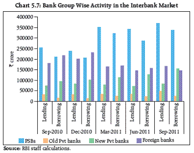
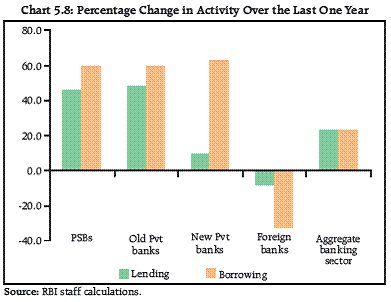
Network Analysis5 5.20 The previous FSR presented the results of the network analysis of the Indian banking system undertaken with a view to gauge the interconnectedness in the banking system and to assess the risks arising out of possible contagion. The analysis has been carried forward to assess the interconnectedness in the entire financial system and to probe further into the nature of the network of the banking system and of the financial system. The purpose is to explore the implications that the structure of the network may have for the stability of the system and vulnerabilities presented by the random failure of one or more different entities in the system. Continuous monitoring of changes in the network structure over time form a critical part of the toolkit for macroprudential surveillance.6 The interbank market grew, but activities of foreign banks fell sharply.... 5.21 The interbank market grew by more than 20 per cent over the one year since September 2010 (Charts 5.7 and 5.8). However, there were some significant changes in the nature of the market, particularly with respect to the activities of the different segments of the market. The quantum of lending and borrowing by foreign banks fell sharply, while that of the other segments increased. The increase in the quantum of interbank borrowing by the new private sector banks was much sharper than the increase in the quantum of their interbank lending.
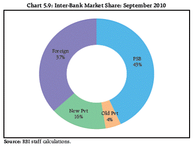
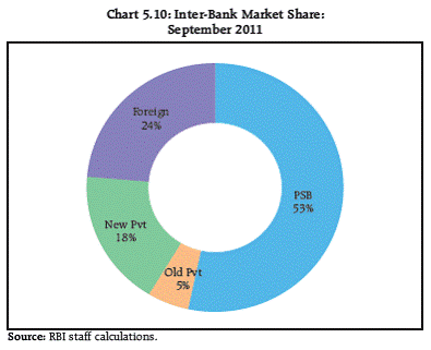
...leading to a fall in their share in the market 5.22 The share of foreign banks in total interbank borrowing and lending activity fell sharply between September 2010 and September 2011, while that of public sector banks increased. There was only a marginal increase in the share of the private sector banks, both old and new (Charts 5.9 and 5.10).
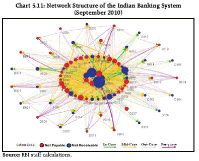
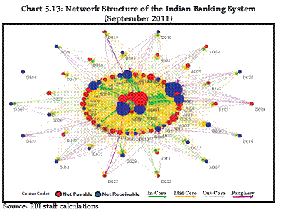
The Indian inter-bank network remains clustered and is also distinctly tiered... 5.23 The previous FSR had found the Indian financial system to be closely connected and clustered. The Cluster Coefficient and Connectivity Ratio in the banking system have consistently remained at over 42 per cent and 28 per cent respectively over the last one year, signifying a high level of interconnectedness in the system. In addition, similar to most interbank and inter-financial systems globally, the network of the system also displays a distinct tiered structure (Box 5.1), which is also persistent over the period (Charts 5.11 to 5.13).
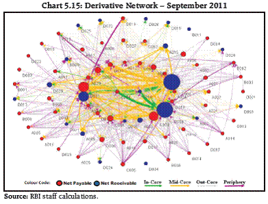
… with implications for the stability of the network though regulatory limits on interbank exposures mitigate contagion risks 5.24 A tiered network structure has financial stability implications. The contagion loss to the system from failure of a bank in the inner core will be more significant than the loss arising out of the failure of the bank in a less tiered network. In the Indian case, however, regulatory limits in interbank exposures mitigate such contagion losses, as was discussed in the previous FSR. Tiered network structure also observed in the interbank derivatives market... 5.25 The network of inter-bank derivatives market also shows a distinct and persistent tiered structure with the major participants in this market being the foreign banks (Charts 5.14 and 5.15). This has been discussed in further detail in Chapter IV of this Report. Box 5.1 Network Analysis Concepts As was discussed in the previous FSR, matrix algebra is at the core of network analysis - an analysis of bilateral exposures between entities in the financial sector. Each institution's lending and borrowings with all others in the system are plotted in a square matrix and are then mapped in a network graph. The nodes (balls) in the graph represent the institutions or entities, with the red balls representing the net borrowers in the system and the blue balls representing the net lenders. The links (in the form of arrows) between the nodes represent the net exposure between any two nodes. Each node or entity in the system is linked to one or more entity/entities. If the node represents a net lender then the link is represented by an arrow in the inward direction (called in degree); whereas if it is a net borrower the link is represented by an arrow in the outward direction (called out degree). The size of the nodes represents the net outstanding position of the entity in the system. The thickness of each link is weighted according to the net position between two entities connected by the link. A series of statistical tools are then used to gauge the level of interconnectedness and activity that exist in the system. Chief among them are (a) Measure of connectivity; (b) Cluster Coefficient; and (c) Eigenvector measure of centrality. (a) Measure of connectivity: This is a statistic that measures the extent of links between the nodes relative to all possible links in a complete graph. For a directed graph, denoting the
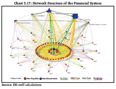
(b) Cluster Coefficient: Clustering in networks measures how interconnected each node is. Specifically, there should be an increased probability that two of a node's neighbours (banks' counterparties in case of the financial network) are also neighbours to each other. A high clustering coefficient for the network corresponds with high interconnectedness prevailing in the system. (c) Eigenvector measure of centrality: Eigenvector centrality is a measure of the importance of a node (bank) in a network. It describes how connected a node's neighbours are and attempts to capture more than just the number of out degrees or direct 'neighbours' a node has. Tiered network structures: Typically, financial networks tend to exhibit a tiered structure. Simply speaking, a tiered structure is one where different institutions have different degrees or levels of connectivity with others in the network. In the present analysis, the most connected banks (based on their eigenvector centrality) are in the inner most core (at the centre of the network diagrams in Charts 5:11 to 5:13). Banks are then placed in the mid core, outer core and the periphery (the respective concentric circles around the centre in the diagrams), based on their level of relative connectivity. The range of connectivity of the banks is defined as a ratio of each bank's in degree and out degree divided by that of the most connected bank. Banks that are ranked in the top 10 percentile of this ratio constitute the inner core. This is followed by a mid core of banks ranked between 90 and 70 percentile and a 3rd tier of banks ranked between 40 and 70 percentile. Banks with connectivity ratio of less than 40 per cent are categorised as the periphery. The colour coding of the links in the tiered network diagram represents the borrowing from different tiers in the network (for example, the green links represent borrowings from the banks in the inner core). The network diagrams show up the peculiar features of a tiered inter bank network in the country. The bulk of the activity takes place between banks in the inner core and the mid core. These banks are closely connected with each other. The banks in the periphery, on the other hand, are connected with the banks in the inner and mid core but have limited exposures to other banks in the periphery. The tiered structure has important implications of financial stability. More concentrated networks like tiered networks are typically less stable. A tiered network structure means that contagion impact of the failure of any bank in the inner or mid core will be much more severe than in the case of a more complete and less concentrated network.
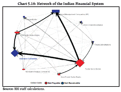
Potential contagion losses increased over the last year signifying heightened systemic importance of the large borrowers 5.26 The contagion tools used to analyse the impact of the random failure of one or more banks were presented in the previous FSR. An analysis of the contagion loss caused to the system by the failure of the top five net borrowers (one at a time) shows that the percentage of the banking system's capital wiped out by the failure of three of these five banks had increased over the last one year. This could be a pointer to greater interconnectedness in the system and also that the systemic importance of the large borrowers may have increased (Table 5.3)7. Mapping the entire financial system...insurance companies and mutual funds are the liquidity providers, public sector banks the major borrowers... 5.27 The network of the entire financial system (including select insurance companies, asset management companies(AMCs), NBFCs, urban banks, financial institutions and scheduled commercial banks) is also tiered and expectedly throws up close interconnectedness especially among the banking, insurance and the mutual funds segments of the financial system. When the entire financial system is mapped, the largest liquidity providers in the system (i.e., the largest net lenders) are the insurance companies and the AMCs while the public sector banks (which are the largest net lenders in the interbank network) emerge as the largest net borrowers in the system accounting for nearly 50 per cent of all borrowing (Table 5.4 and Charts 5.16 and 5.17).
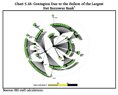
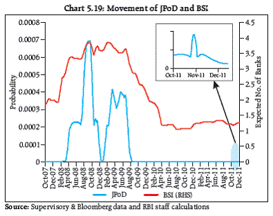
... leaving the liquidity providers vulnerable to any disturbances in the banking system 5.28 The degree of interconnectedness in the financial system (as discussed above) clearly means that the potential contagion loss to the entire financial system arising out of the random failure of one or more large net borrowers in the system would be significantly larger than that of the loss to the banking system alone. In particular, the random failure of a bank which has large borrowings from the insurance and mutual funds segments of the financial system may have significant implications for the entire system. A contagion analysis simulating the failure of one such large borrower (Chart 5.18) could cause distress to ten other institutions, including three insurance companies8. Banking Stability Measures and Estimation of Expected Shortfall 5.29 During times of distress, the fortunes of banks typically decline concurrently through direct or indirect links which include mark-to-market asset values, inter bank lending and information asymmetries. In this section, the results of modelling distress dependencies among banks are presented. For the purpose, the financial system has been conceptualised as a portfolio of a specific group of banks (Segoviano and Goodhart, 2009). In particular, the Banking System's Portfolio Multivariate Density (BSMD)10, which characterises both the individual and joint asset value movements of the portfolio of banks, is recovered from Probabilities of Distress (PoDs) of the banks under analysis. The PoD is observed empirically based on 99.5 per cent Value at Risk (VaR) of banks' daily equity price return. Common distress in the system: JPoD and BSI 5.30 The probability of distress of entire banking system, as measured by Joint Probability of Distress (JPoD), is observed to be very low during the recent period. The other measure of common distress in the banking system is the Banking Stability Index (BSI) (which measures the expected number of banks that become distressed given that at least one bank becomes distressed). The BSI has been hovering around one since April 2010 implying that the banking system has very weak inter-dependency at present. However, it may also be observed that BSI, which was flat during last year, has again started showing a marginal upward movement in the current year (Chart 5.19).
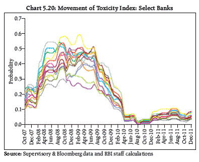
Distress among specific banks: Toxicity and Vulnerability Index 5.31 The distress among the specific banks is measured based on Toxicity Index (TI) and the Vulnerability Index (VI). The TI is the average probability that a bank under distress may cause distress to another bank in the system. Toxicity of banks declined significantly from around 60 per cent registered during the crisis to 5 per cent in the recent period. It may also be mentioned that the TI which had registered a marginal increase during first half of 2011 has shown a downward trend since August 2011 (Chart 5.20).
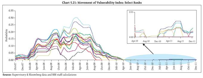
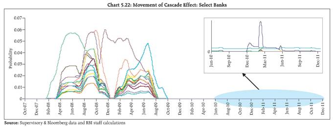
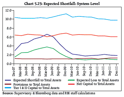
5.32 The VI, which quantifies the vulnerability of a bank given distress in other banks in the system, was high during the financial crisis of 2007-09. The highest probability was about 30 per cent during the crisis, which declined substantially and is hovering very close to zero since June 2010. Of late, VI has shown a little upward movement (Chart 5.21). Distress in the System Associated by Distress in a Specific Bank: Cascade Effect 5.33 Distress in the system associated by distress in a specific bank, representing the likelihood that the entire system becomes distressed is useful to quantify the systemic importance and 'domino' effect of a specific bank's distress. At present, domino impact for failure of the entire banking system is quite low (Chart 5.22). Expected Shortfall 5.34 The banking system's Expected Shortfall (i.e. the estimated loss of assets in the extreme loss region) has been declining continuously in recent periods - from around 6.6 per cent of total assets of banking system in March 2009 to only 1.8 per cent in December 2011 implying that the banking system would be able to withstand the extreme systemic losses as derived from the model (Chart 5.23).
Macrofinancial Stress Testing 5.35 Two sets of macro testing exercises were conducted: one based on multivariate regression and the other on vector autoregressive (VAR) model. The former allows evaluating the impact of a particular macroeconomic variable on the banking system's capital and non-performing advances (NPA) ratio. The latter reflects the impact of the overall economic stress situation on the banks' capital and NPA ratio taking into account the feed-back effect. The impact on systemic risk is judged through various models to understand the impact of macroeconomic variables from different but complementary angles. The stress scenarios 5.36 The macro stress tests used a baseline and three adverse macroeconomic scenarios; low risk, medium risk and severe risk (Table 5.5), for which projections were based on the data till Q2: FY2011-12. These shocks have been calibrated based on historical data.
Modeling credit risk using a series of econometric models 5.37 Credit risk was one of the key focus areas for the macro-stress tests. Credit risk stress tests have been designed using several econometric models11 that relate banking system aggregates to the macroeconomic variables, such as (i) multivariate logit regression on aggregate systems' NPA data; (ii) multivariate regression in terms of the slippage ratio (inflow of new NPAs); (iii) aggregate VAR using slippage ratios; (iv) multivariate panel regression on bank wise slippage ratio data, which was later aggregated into bank-groups; and (v) multivariate regressions for aggregate sectoral NPAs. The banking system aggregate includes current and lagged values of aggregate NPAs (NPA ratio) and inflow of new NPAs (slippage ratio), while macroeconomic variables include GDP growth, short term interest rate (call rate), WPI inflation and export-to-GDP ratio. Risk scenarios are constructed from the above table, where the shocks in the major macroeconomic parameters occur simultaneously. The stress tests were run on the unconsolidated balance sheet data of banks for their domestic operations. 5.38 The stress tests models were built on the quarterly data from June-2001 to Sep-2011. The dependent variable for the aggregate multivariate and bank wise panel regressions, as well as VAR was the slippage ratio, whereas, the dependent variable for logit regression and sectoral data was NPA ratio. System level credit risk tests: Projected NPA increases, impact on CRAR is contained 5.39 The results of the aggregate credit risk exercise provide a broad indication of potential impacts. The gross NPA ratio projections through different models (Table 5.6) suggest that the aggregate banking system gross NPA ratio, which is expected to be between 3.2 to 3.5 per cent by March 2013 under baseline scenario as projected by different models, may attain a high level of 4.7 to 5.8 percent under severe risk scenario. The projected level of NPAs based on VAR is more than that based on multivariate regression, as the VAR model also takes into account feed-back effect and in addition, the initial shock will remain in the system for the six quarters' horizon, unlike the multivariate regressions, where it dies out gradually. However, the impact on CRAR is contained (Table 5.7).
Bank group level credit risk: Foreign banks most impacted, but CRAR is resilient 5.40 The effect of the risk scenarios varies by bank groups. The maximum impact on NPAs is observed for foreign banks, because of their relatively small and fewer commercial loans. There is a big difference in NPAs of these banks in the baseline and severe risk scenario compared with other bank groups (Table 5.8). 5.41 Aggregate credit risk, as measured by the change in CRAR, shows that foreign banks are affected the most, followed by other bank groups (Table 5.9). In the severe risk scenario, the average CRAR of foreign banks declined by 287 basis points in the next six quarters to 13.4 per cent, but remains well above the regulatory requirement. Public sector banks and old private banks would also experience similar impact in their loan portfolios under severe stress scenario, which may bring down the CRAR of these groups. However, the CRAR remains above the regulatory requirement even under the severe risk scenario. Sectoral credit risk: Impact on Food Processing, Engineering and Iron & Steel sectors relatively high 5.42 Sectoral credit risk, as measured by changes in NPAs, revealed that among eight main sectors, Food Processing, Engineering and Iron & Steel sectors appear to be affected the most (Table 5.10). The effect on NPAs in Agriculture in this macro stress test analysis seems to be marginal. Similar effect is observed for the NPAs in infrastructure.
Concluding Remarks 5.43 The series of measures put in place to assess systemic risks in the financial system are aimed at capturing the different types of systemic events and risks through a variety of modeling frameworks. 5.44 The Systemic Risk Survey provided the inputs of a large cross section of market participants on risks to systemic stability. The respondents identified deterioration in the asset quality of banks as the most significant risk to the financial system followed by risks from heightened market volatility, including exchange rate volatility, global risks, risks from high inflation and high interest rates. They remained, however, reasonably confident about the stability of the Indian financial system. The Systemic Liquidity Indicator shows that liquidity conditions have become tighter in recent months. The network of the Indian banking and financial system have a tiered structure but limits on inter bank liabilities mitigate contagion risks. Distress dependencies between banks continued to be low. 5.45 The series of systemic risk assessment initiatives set out in this FSR are a critical part of the overall system of macroprudential surveillance which attempts to identify, measure and manage, including, if necessary, through preemptive policy action, burgeoning vulnerabilities and excesses. However, this is easier said than done both because of the intrinsic complexities of systemic risks and also since the theoretical and empirical research on systemic risk is still in its early developmental stage. All of this indicate that it would be un-realistic to expect a single measure of systemic risks to cater to all kinds of risks or even to a single kind of risk with precision at all times. This, in turn, creates the need for macroprudential authorities to "build up, from scratch, a wide range of measures and tools covering different aspects of systemic risk in different parts of the financial system, with each tool having its specific purposes, advantages and caveats that must always be borne in mind when interpreting its results"12. The series of models / measures presented in this Chapter as well as the series of stability indictors/ maps presented in the other Chapters of this Report represent the efforts within the Reserve Bank to assess systemic risks from different dimensions and perspectives. 1 "Seeing Both the Forest and the Trees-Supervising Systemic Risk", Jose Vinals, IMF Financial Counsellor and Director, Monetary and Capital Markets Department Opening Remarks at the Eleventh Annual International Seminar on Policy Challenges for the Financial Sector Washington D.C., June 2, 2011. 2 The bars in the chart represent the weighted aggregate of the number of respondents who have identified the corresponding risk, the weights representing the probability assigned by the respondent to the occurrence of the risk. 3 The methodology is given in the Annex to this Report. 4 "Measuring Financial Stress in a Developed Country: An Application to Canada", by Mark illing and Ying Liu (2006). 5 The network analysis has been conducted based on data in respect of bilateral fund based and non-fund based exposures between banks, asset management companies, insurance companies, NBFCs, financial institutions and urban cooperative banks on different dates. The transactions where the settlement takes place through a central counterparty have not been reckoned. 6 The Network model used in the analysis has been developed by Professor Sheri Markose (University of Essex) and Dr. Simone Giansante (Bath University) in collaboration with the Financial Stability Unit, Reserve Bank of India. 7 The five banks on each date discussed above are the top five net borrowers on that particular date. 8 Distress conditions for banks and NBFCs are defined based on their capital adequacy ratio, while for insurance companies it is based on the solvency ratio. Conceptually an AMC will not fail as such due to a contagion event, since it will simply pass on the losses to all the unit holders. 9 Colour code:
(i) Green: Institutions which are affected by the failure of the trigger/distressed institutions but which are able to absorb the shock. (ii) Yellow: Banks which are affected by the failure of the trigger/distressed banks and whose capital adequacy falls below 9 per cent but core capital ratio remains above 6 per cent 10 Details are in FSR-June 2011. 11 The methodology is given in the Annex to this Report. 12 "Implementing a macroprudential framework: Blending boldness and realism" Claudio Borio. Bank for International Settlements, July 2010. |
||||||||||||||||||||||||||||||||||||||||||||||||||||||||||||||||||||||||||||||||||||||||||||||||||||||||||||||||||||||||||||||||||||||||||||||||||||||||||||||||||||||||||||||||||||||||||||||||||||||||||||||||||||||||||||||||||||||||||||||||||||||||||||||||||||||||||||||||||||||||||||||||||||||||||||||||||||||||||||||||||||||||||||||||||||||||||||||||||||||||||||||||||||||||||||||||||||||||||||||||||||||||||||||||||
પેજની છેલ્લી અપડેટની તારીખ:


