by Renjith Mohan, Saquib Hasan, Sayoni Roy, Suvendu Sarkar, and Joice John^{^}

This article attempts to develop a methodology for forecasting the headline Consumer Price Index (CPI) inflation as well as CPI excluding food and fuel inflation for India using various statistical, machine learning, and deep learning models, which are then combined using a performance-weighted forecasts combination approach. This framework can also be used to generate density forecasts and can provide estimates of standard deviation as well as the asymmetry, around the weighted average inflation forecasts. The results indicate a clear advantage in using all model classes together. It is also seen that a performance-weighted combination of statistical, ML and DL models leverages the strengths of each approach, resulting in more accurate and reliable inflation forecasts in the Indian context.

Introduction

Inflation forecasts are a key set of information for the conduct of monetary policy in Inflation Targeting (IT) central banks as forward-looking policies would have to take into account conditional predictions of various key macroeconomic variables given the lags in transmission and other nominal rigidities. It is also important to assess and communicate risks around those predictions, which helps in building credibility and improving transparency. Acknowledging that no single model can capture all economic complexities, central banks around the globe generally adopt a ‘Suite of Models’ approach, integrating diverse frameworks to improve the predictive accuracy. Traditionally, models that are dependent on macro and/or micro economic theories detailing the complex macroeconomic relationships have often been used in most central banks for informing the policy decision-making. More recently, with the advancement in computational capacity, large-scale statistical and Machine Learning (ML) models are also becoming popular. While traditional models attempt to predict the macroeconomic outcomes from the interactions of economic agents, ML and Deep Learning (DL) models are more data-dependent and focus more on the state of the economy. In practice, both can function in complementarity to provide valuable information to the policy makers. Traditional statistical models are useful for their stability¹ and interpretability, whereas ML models may offer advancements in forecast accuracy. However, its inability to provide a coherent interpretation remains a concern.

In this context, this article attempts to a develop a ‘suite’ of statistical and ML models for forecasting CPI headline and core inflation² in India. It attempts to synthesise two earlier works done in the Indian context viz. Bhoi and Singh (2022) which focused on ML models for inflation forecasting, and John et al. (2020) which explored the forecast combination approach using different time series and statistical models for forecasting CPI inflation. While Bhoi and Singh (2022) found relative gains in using ML-based techniques over traditional ones in forecasting inflation in India, John et al. (2020) established the relative advantage of using forecast combination approaches for inflation forecasting in India.

Building on these results, this article employs a combination approach for forecasting CPI headline and core inflations in India, generated from a large number (say 216) of statistical, ML, and DL models³, and evaluates its pseudo-out of sample⁴ forecast performance. Availability of large number of individual forecasts enable this framework to sum up those into density forecasts and hence can also be used to estimate the standard deviation and skewness. The article is structured as follows: Section 2 reviews the relevant literature; the data and methodologies are outlined in Section 3; Section 4 discusses the empirical results; and concluding remarks are put together in Section 5.

2. Literature Review

With the increase in computational power over the years, as shown in Bates and Granger (1969), the world has shifted from using a ‘single best model’ approach to ‘forecast combination’ approach, thereby, overcoming the uncertainties arising from usage of different datasets, assumptions and various specifications of the models thus, by increasing the reliability of the results.

Stock and Watson (2004) employed the benefits of combination techniques to macroeconomic forecasting, particularly for output growth across seven countries. They found that simple methods such as averaging multiple forecasts, often outperformed more complex and adaptive techniques, and aided to mitigate the instability often seen in individual economic forecasts. Their findings underscored the point that complexity in forecasting models does not necessarily result in better accuracy, especially in uncertain environments. They found that forecasts from even simple combination approaches proved more accurate than sophisticated models in many cases.

The “M” competitions initiated by Spyros Makridakis in 1982 have had a colossal impact on the forecasting sphere. Instead of focusing on the mathematical properties of the models (which was the traditional way of looking at the forecasting models), they paid sole attention to out of sample forecast accuracy. They found that complex forecasting models do not necessarily always offer more precise projections than simpler ones. Following the legacy, the “M4” competition, launched in 2017, tested a range of methods, including traditional statistical models like Auto-Regressive Integrated Moving Average (ARIMA) and Exponential Smoothing (ETS) alongside various ML and DL models. A key takeaway from the competition was that simple combination methods, such as Comb⁵—a straightforward average of several ETS variants—outperformed more advanced techniques across various data frequencies. This reinforced the idea that simpler methods often outperform more sophisticated models. The competition also revealed the limitations of pure ML models, which at times underperformed to traditional statistical methods. This highlighted the need for a hybrid approach that combines ML/DL algorithms and traditional statistical methods in a forecast combination framework to improve overall forecasting accuracy.

In the Indian context, John et al. (2020) explored inflation forecast combination approach in the Indian context, using 26 different time series and statistical models, but not including ML and DL approaches. Their study emphasised the value of traditional econometric methods while acknowledging the growing importance of ML and DL models. John et al. (2020) further pointed to the need for an integrated approach that combines the forecasts from individual models to enhance the forecasting accuracy. Bhoi and Singh (2022) focused on refining econometric models for inflation forecasting in India, stressing the enhanced performance of ML/DL models for forecasting CPI inflation in the Indian context.

3. Data and Methodology

3.1 Data

The time-series CPI data released by the National Statistical Office (NSO) for the period January 2012 to July 2024 has been used as the primary (dependent) variable of interest. Apart from headline inflation, core inflation (derived from CPI by excluding food and fuel) is also separately modelled for generating forecasts using the same methodology. The other explanatory variables used as the determinants of headline and core inflations in various models are – (i) crude oil price (Indian basket), (ii) Rupee-United States Dollar (INR-USD) exchange rate, (iii) real gross domestic product (GDP) and output gap⁶ and (iv) policy repo rate⁷.

3.2 Methodology

A large number of h-period ahead inflation forecasts are generated using various statistical, ML, and DL models, which are then aggregated using weights that are being derived based on the out of sample forecast performance of these models. The detailed steps for estimating the inflation forecasts using performance-weighted combinations are as under:

i. Inflation series are seasonally adjusted using the X-13 ARIMA⁸ technique.

ii. Exogenous variables like INR-USD, Indian basket of crude oil price, real GDP and output gap are used for the estimations in some models. The series which are available only on quarterly frequency (GDP and output gap) are converted to monthly frequency using the temporal disaggregation method⁹.

iii. Seasonally adjusted annualised rates (SAAR) of CPI (headline and core, separately) are then calculated.

iv. Two different window sizes are used for the estimation – 36 months (3 years) and 96 months (8 years). These windows are rolled over for the entire sample period. This produced multiple sub-samples of data. A shorter window size of 3 years and a longer window size of 8 years are used to minimise the bias emanating from a fixed sample size.

v. Each model in Table 1 is estimated separately in each sub-sample using SAAR (headline and core, separately) as the dependent variable (or as one of the dependent variables).

viii. The 12-month ahead root mean squared forecast error (RMSE) for the model i is estimated using the following formulae. A window size of 12 months has been used to calculate the RMSEs. These are estimated for each subsample.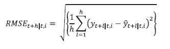

ix. The weights for the forecast combination are estimated as follows: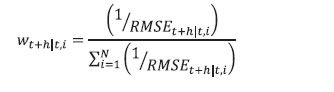

where, N is the total number of models.

x. These weights are used to calculate the weighted average of inflation forecasts from the individual models.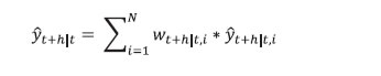

xi. Furthermore, 216 different inflation point forecasts for each horizon are bifurcated in two groups – (a) above the weighted average forecast, (b) below the weighted average forecast. Then, the RMSE-weighted standard deviation is calculated for both groups (σ₁ and σ₂, where σ₁ is the standard deviation of the forecasts above the weighted average forecast and σ₂ is the standard deviation of the forecasts below the weighted average forecast).

xii. Assuming a split-normal distribution asymmetric confidence intervals of desired significant levels can be calculated around each h-period ahead forecasts.

xiii. Finally, the asymmetry of the forecast can be determined using the formulae:

3.3 Toolbox / Software

The entire methodology described above has been programmed and a toolbox has been developed in MATLAB.

4. Empirical Findings

4.1 Estimated Inflation Forecast, Standard Deviation and Asymmetry: An Illustration

The 12-month ahead performance-weighted inflation forecasts, standard deviation and asymmetry, which are estimated using the suit of models generated using the data till December 2023 is presented in Chart 1.

The realised monthly inflation numbers for 2024 forecasted using the data till December 2023 fell well within the range of forecasts and was broadly aligned with performance-weighted forecasts. As expected, the standard deviations were higher for longer horizons. The asymmetricity was pointing towards an upward bias in the forecast. The comparison of the forecast accuracy of the performance-weighted forecasts vis-à-vis that of the individual models and the simple average forecasts for the entire sample period is carried out in the following sub-sections.

4.2 A Comparison of RMSEs: Individual Models Versus Performance-weighted:

The average RMSE across the 12-month horizon of the performance-weighted forecasts for the headline and core inflation are found to be approximately 70 per cent lower than the benchmark random walk (RW) forecast. It is also found to be better than the forecasts generated by more than 75 per cent of models in all horizons. Certain models produce better forecasts in some horizons and for some windows. The best performers are not the same throughout all the horizons as well as for all the windows. However, a judicious combination of forecasts (like performance-weighting) helps to reduce biases arising out of such divergences (Charts 2 & 3). Unlike what witnessed for core inflation forecasts, the plateauing nature of the RMSEs for headline inflation forecasts as horizon increases may be due to the influence of the effect of the transitory shocks.

4.3 Forecast Accuracy¹⁰: Performance-weighted Versus Simple Average

The Diebold-Mariano (DM)¹¹ test has been used for a formal statistical comparison of the performance-weighted combination method from that of a simple average forecast for each class of models (Statistical, ML and DL) as well as for the entire basket of all 216 forecasts, separately, over different forecast horizons.

In the DM test, the null hypothesis is that the simple average is as accurate as the performance-weighted forecast combinations, while the alternative hypotheses are: (i) the simple average is less accurate than the performance-weighted combination, and (ii) the simple average is more accurate than the performance-weighted combination. To minimise the ‘size bias’ in small samples, the bias correction suggested by Harvey, Leybourne, and Newbold (1998) was applied, using Student’s t critical values instead of standard normal values. Table 2 presents the results for four forecast horizons, applied separately to two different rolling window sizes for both headline and core inflation. The DM test was performed separately for each model type — Statistical, ML, DL, and a combination of all models — for headline and core inflation, as well as for each rolling window size. This resulted in sixteen instances (forecast horizon (4) x model types (4)) for each combination of window size and inflation type.

Overall, the performance-weighted forecasts for both headline and core inflations were found to be at par or better than simple average forecasts for all model classes and across horizons, attaching a minimum guarantee of forecast accuracy for the performance-weighted forecasts. The comparison between the two aggregation methods for headline inflation using a rolling window of three years (column (1) in Table 2) revealed that the performance-weighted method significantly outperformed the simple average method in 12 out of 16 instances. However, with a rolling window of eight years for headline inflation, the performance-weighted method only outperformed the simple average in two cases (out of 16) (column (2) in Table 2). On the other hand, simple average forecasts did not significantly outperform the performance-weighted in any cases. For core inflation, the performance-weighted method surpassed the simple average in six and four cases (out of 16) for window sizes of three and eight years, respectively (columns (3) and (4) in Table 2). Notably, the simple average never significantly outperformed the performance-weighted method. To reiterate the results, RMSEs for the simple average and performance-weighted forecasts are compared using the paired Wilcoxon signed-rank test¹² (Table 3).

Table 3 compares the RMSEs of simple average forecasts versus performance-weighted forecast averages of headline and core inflations, under different model classes and rolling window sizes. The null hypothesis is that the RMSE of the simple average forecast is as accurate as that of the performance weighted one, with the alternatives being that the simple average is either more or less accurate. Results show that the RMSE of the performance-weighted forecast average is significantly lower than that of the simple average on a consistent basis, reinforcing the DM test findings in Table 2 that performance-weighted combinations yield more or similarly accurate inflation forecasts than that of simple average forecast in the Indian context.

4.4 Forecast accuracy of performance-weighted forecasts among various classes of models

After confirming the efficacy of the performance-weighted forecast over the simple average forecast, now we turn towards the comparison of the forecast performance of the weighted average forecasts across different classes of models viz. Statistical, ML, DL, and the super-class of all models. First, using the DM test, the forecast accuracy of the individual model classes (statistical, ML and DL) – aggregated using performance weights – is compared with the all-models combined forecasts, which aggregates the forecasts from all 216 individual models using performance-weighted weights. The DM test is applied across different forecast horizons, rolling window sizes, and for inflation categories (headline and core).

The results show that for the 3-year rolling window, the all-combined forecasts significantly outperform the performance-weighted forecasts from different class of models in four out of 12 instances, for both core and headline inflation (columns (1) and (3) in Table 4), while for others all-combined forecasts are at par across different class of models. However, for an 8-year rolling window, the all-combined forecasts perform better in only one case (columns (2) and (4) in Table 4). More importantly, weighted forecasts from neither of the model classes (statistical, ML or DL) in both horizons or for either headline or core inflations, significantly outperformed the all-models combined forecasts (Table 4). When each model class is analysed separately vis-à-vis the all-models combined, performance-weighted forecast significantly outperformed the weighted forecast from the class of DL models in most instances (six out of eight) but performs mostly similarly to that from statistical and ML models.

The paired Wilcoxon signed-rank test supports these findings, showing that the all-models combined forecasts outperformed the weighted forecasts from statistical models in most cases. Further, the accuracy of the all-models combined forecasts is found to be at par with the forecast combination derived separately from ML and DL models.

5. Concluding Remarks

The findings strongly support the effectiveness of forecast combination of statistical, ML and DL methods in improving inflation forecasting accuracy in the Indian context. The results indicate a clear advantage in using all model classes together, with a guarantee that the forecast accuracy never deteriorate while combining forecasts from all classes of models and getting better in most cases. It further reiterates that a performance-weighted combination of statistical, ML and DL models leverages the strengths of each approach, resulting in more accurate and reliable inflation forecasts in the Indian context. Additionally, forecast combination approach provides a confidence band that allows policymakers to assess risks and make more informed decisions.

This approach is particularly valuable in the Indian context given the complexities of its inflation dynamics, which is often influenced by global uncertainties and food price volatility. However, it is crucial to acknowledge that there are time-variations, asymmetries and nonlinearities that influence the inflationary developments emanating from overlapping shocks. Even then the combination of forecasts generated from statistical, ML and DL models ensures robustness, as it minimises the model misspecifications biases, making it a much more reliable benchmark.

References:

Bates, J. M., & Granger, C. W. (1969). The combination of forecasts. Journal of the Operational Research Society, 20(4), 451-468.

Denton, F. T. (1971). Adjustment of monthly or quarterly series to annual totals: an approach based on quadratic minimization. Journal of the American Statistical Association, 66(333), 99-102.

John, J., Singh, S., & Kapur, M. (2020). Inflation Forecast Combinations: The Indian Experience. Reserve Bank of India Working Paper Series No. 11.

Makridakis, S., Spiliotis, E., & Assimakopoulos, V. (2020). The M4 Competition: 100,000 time series and 61 forecasting methods. International Journal of Forecasting, 36(1), 54-74.

Singh, N., & Bhoi, B. (2022). Inflation Forecasting in India: Are Machine Learning Techniques Useful?. Reserve Bank of India Occasional Papers, 43(2).

Stock, J. H., & Watson, M. W. (2004). Combination forecasts of output growth in a seven-country data set. Journal of Forecasting, 23(6), 405–430. https://doi.org/ https://doi.org/10.1002/for.928

Harvey, D. I., Leybourne, S. J., & Newbold, P. (1998). Tests for forecast encompassing. Journal of Business & Economic Statistics, 16(2), 254-259.

Annex

^{^} The authors are from the Department of Statistics and Information Management (DSIM), Reserve Bank of India (RBI). The views expressed in this article are those of the authors and do not represent the views of the Reserve Bank of India.

¹ Stability here implies the robustness of model forecasts against variations in hyperparameter tuning. Unlike traditional statistical models, which rely on well-defined parametric structures, ML and DL models often exhibit sensitivity to hyperparameter choices, leading to forecast volatility across different tuning configurations.

² CPI excluding food and fuel. This notion is used in the rest of the article

³ Statistical models are structured mathematical framework-based model built on probability theory and assumptions about data generating process. ML models are data-driven algorithms that identify patterns and optimise predictions without strict parametric assumptions. DL models are subset of ML models where multi-layered neural networks are employed to extract hierarchical representations from large datasets for complex tasks.

⁴ In a pseudo out-of-sample forecasting exercise (usually conducted ex-post the availability of the actual data for verifying the forecastablity of the framework), the forecasts are generated at some time t in the past, using only the data available till that time for the parametrisation of the model as well as for generating the forecast of exogenous variables.

⁵ Comb model is the simple arithmetic average of single exponential smoothing, Holt and damped exponential smoothing.

⁶ Output gap is defined as (actual GDP level minus potential GDP level)*100/(potential GDP level). Potential GDP is estimated by using Hodrick-Prescott (HP) filter.

⁷ Crude oil prices (Indian Basket) are obtained from the Petroleum Planning & Analysis Cell (PPAC) under the Ministry of Petroleum & Natural Gas, Government of India (GoI). Real Gross Domestic Product data is sourced from the Ministry of Statistics and Programme Implementation (MoSPI), GoI. The INR-USD exchange rate and the repo rate are sourced from the Database of Indian Economy (DBIE) maintained by the Reserve Bank of India (RBI).

⁸ X-13 ARIMA uses Seasonal ARIMA (SARIMA) models to determine the seasonal pattern in the economic series. The order of the SARIMA models is determined based on the in-sample goodness of fit of different models and the best model is selected using suitable information criteria. The selected model, therefore, represents the underlying data-generating process through average parameter estimates.

⁹ Temporal disaggregation has been carried out using Denton-Cholette method (Denton, 1971).

¹⁰ Root Mean Squared Error (RMSE) is mostly used as the metric of the accuracy of forecasting models. Lower RMSEs indicates better accuracy of the forecast. This notion is interchangeably used in this article.

¹¹ DM Test compares forecast accuracy between two models and test whether the difference in forecast errors between two models is statistically significant.

¹² This non-parametric test is useful for comparing two matched samples, providing a robust alternative to the paired t-test when the focus is on comparative performances. The test assesses whether there is a greater-than-50 per cent probability that RMSEs of the performance-weighted average forecasts of 1-month to 12-month ahead horizon from a particular class of model is greater than that from the other classes, separately.