 IST,
IST,


III Exploring The Slowdown (Part 1 of 3)
Macroeconomics of Growth
Structural Constraints in Indian Agriculture
Introduction
3.1 The recent deceleration in the Indian economy has generated considerable concern with some apprehensions about the deepening of the slowdown and delay in revival. Several factors are attributed to the loss of growth. Infrastructural constraints, variability and shortfalls in agricultural output, erosion in the quality of public services and gaps in technology and human development are insidiously becoming binding constraints on growth. At the same time, recent developments indicate some cyclicity in output behaviour with the current phase of the cycle reflecting the general deficiency in aggregate demand, the inadequate response of private investment to reforms, deceleration in public investment, inventory accumulation, excess capacity and some evidence of consumption smoothing. In the current year, indicators of real activity, with the exception of agriculture, have underperformed in relation to the preceding year. A few positive signs are, however, visible in the improved capitalflows and the steady build-up in the foreign exchange reserves. The principal policy, instruments, i.e., fiscal and monetary policies have been shifted into counter-cyclical mode and the stance of policies is clearly in favour of further adjustments, if necessary, to create a congenial environment for the awaited upturn. There is also a growing recognition that the existing level of structural reforms is succumbing to the inexorability of diminishing returns, and bolder and more intensified reforms are required in the 'difficult areas' - agriculture, labour market, bankruptcy and exit procedures, social sector and legal reforms.
3.2 The persistence of the slowdown for the second year in succession has provoked intense debate on the underlying causes of the downturn. Although the views traverse a wide spectrum, a broad categorisation helps to place the debate in proper perspective.
3.3 There is an influential viewpoint which attributes the deceleration to forces operating on demand such as, low aggregate demand and adverse investment climate (NCAER, 2001), the sharp deceleration in the two major components of industrial demand-exports and investment (Acharya, 2001), the contractionary features inherent in public policies pursued in the 1990s (Shetty, 2001), and specifically, anti-cyclical fiscal policies, and the inappropriate budgetary stance (Rakshit, 2000). All of the above are reflective of a demand-constrained economy (Patnaik, 2001). Within the 'demand constraint' side of the debate, there is also the view that the declining trend in growth is to be attributed to demand recession as well as global slowdown (Institute of Economic Growth, 2001). The impact of contemporaneous global developments has also been emphasised as the overwhelming reason; one view cautions the government to be ready to handle the adverse consequences of continuing global slowdown (Venkitaramanan, 2001), while another suggests that 'the government can do very little about it' (Economic Times, 2001). The contrarian viewpoint argues that the impact of the global slowdown on the domestic output growth may be minimal and the current phase may be temporary (Bhalla, 2001; Bhattacharya, 2001; Rao, 2001).
3.4 The other side of the debate ascribes the slowdown to factors operating primarily on aggregate supply. The slide in the pace of growth is attributed essentially to the growth of the commodity producing sectors- agriculture and manufacturing (Chandrasekhar, 2001). Pointing to the institutional impediments to growth, it is argued that the main reasons for the current slowdown are structural and should be addressed accordingly (Karnik, 2001). The slowing down of growth is also regarded as reflecting the effects of various shocks, such as, the Asian financial crisis, international oil prices, 'patchy' monsoon and natural calamities along with deeper structural factors at work, including infrastructure constraints, regulatory constraints in industry, agriculture and trade, and high real interest rates (IMF, 2001) as well as slow pace of reforms (International Finance Corporation, 2001). The current decelerating phase is also associated with relatively high unemployment, poor human and social development and ecological degradation (GoI, 2001). Finally, there is the view that the recent slowdown in economic activity seems to reflect a combination of both cyclical and structural factors with different weights assignable to either, depending on the changing conditions in the growth process (Reserve Bank of India, 2001).
3.5 Against the backdrop of the current deceleration, the impassioned debate generated in India and the diversity of views about the downturn, this Chapter undertakes an analytical examination of the dynamics of India's growth performance. The approach is exploratory and empirical with the objective of presenting the findings of a series of integrated analytical exercises on various facets of the deceleration for contributing to informed public judgement and choice. The following section deals with the macroeconomics of growth, in terms of aggregate demand and cyclical influences thereon, factors underlying the behaviour of aggregate demand such as consumption, saving, investment and net exports. Sections II and III address specific structural constraints on aggregate supply in agriculture and industry, respectively. Section IV examines the role of services as a lever of growth. Section V profiles the regional dimensions of the growth process. This is followed by concluding observations.
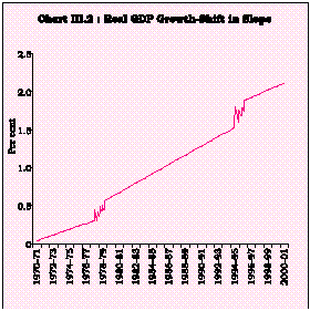
3.6 As a starting point, it is useful to date the important turning points in the time path of the Indian economy. Real GDP at factor cost represents a summary measure of economic performance. The growth profile of real GDP in India has not been smooth and evenly paced. The Markov-switching model (Goldfeld and Quandt, 1973) can be employed to capture the dynamic patterns underlying switches or shifts in regimes which are independent over time. This procedure represents an improvement over the conventional techniques that rely on prior knowledge of the existence of those shifts. The exercise reveals that the growth of GDP encountered the first 'break' in 1981-82 followed by a second 'break' in 1990-91. The first break occurred in the wake of the second oil shock and a severe drought. The response to these supply shocks resulted in a step-up in the growth process with the trend growth rate rising from 3.4 per cent during 1970-81 to 5.6 per cent during 1981-90. The second break is detected amidst the unprecedented balance of payments crisis associated with the Gulf war in 1990. In a similar sequence, the simultaneous implementation of structural reform and stabilisation brought about a quantum jump in the trend growth to 6.5 per cent in the ensuing years (Chart III.1).
|

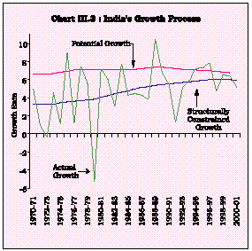
3.7 There is no evidence of a structural break in the trend growth during the 1990s when judged from levels; however, the growth process has also been subject to variations in pace as indicated by the recent downturn. Using the switching regression technique which employs consecutive trial searches over the entire sample period to identify acceleration/ deceleration in real GDP growth in terms of rates of change, an inflexion is discernible in 1978-79 showing an acceleration and again in 1995-96 with the wearing-off of the preceding high growth phases. These experiences suggest that the current phase represents a loss of speed rather than a 'break' in growth (Chart III.2).
|
3.8 Taking the diagnosis further, an incision can be made into the growth path of real GDP by decomposing it into its 'time-series' components - trend, seasonal, cyclical and irregular elements-depending upon the frequency and regularity of their recurrence. Seasonal components are discernible in monthly and quarterly data but not in the annual data. The cyclical and irregular components are collected together and removed by 'filtering' real GDP through the commonly employed Hodrick-Prescott (HP) filter over the period 1970-71 to 2000-01. Separating out cyclical and irregular influences from the actual growth of real GDP yields what can be termed as the 'structurally constrained' growth path of the economy determined by its production structure, institutional characteristics and the various impediments acting on aggregate supply. The path of structurally constrained growth has undergone a distinct upward shift in the early 1990s as liberalisation unlocked hidden capacities and unleashed repressed productive forces. In the following years, the impetus for growth was not sustained and the structurally constrained path tended to slope downwards in the second half of the 1990s. These movements have had a fundamental influence on the potential growth path of the Indian economy, i.e., the growth which is realisable with the full utilisation of productive capacities in the economy. Empirical studies conducted in India show the sensitive nature of the estimates of potential growth to the choice of methodology (RBI, 1999). Applying the OECD (1995) method, the potential growth path is generated from the actual data on real GDP by obtaining a locus of the peak growth rates achieved in the period of study and then smoothing it with a three-year moving average. Movements in the potential growth are found to respond to the behaviour of the structurally constrained growth path. The liberalisation 'hump' of the early 1990s shifts the potential growth path upwards; again the dipping of the potential growth path appears to be associated with the slowing down of structurally constrained growth (Chart III.3). Thus, by releasing the structural constraints, it is possible to shift the long run growth to a higher trajectory.
|
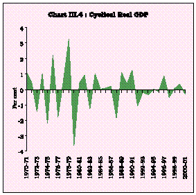
3.9 The exercise also provides some insights into the characteristics of cycles in the Indian economy. Cyclical and irregular components (which were jointly separated by using the HP filter) are disentangled further by using a conventional business cycle filter, i.e., the Band-Pass filter (Baxter and King, 1999) which produces a smooth cycle by eliminating the outliers over the 'band' of frequencies. The cyclical component of real GDP is depicted in Chart III.4. Its behaviour suggests that during the 1970s and early 1980s, cyclical fluctuations were frequent and sharp in magnitude, varying in the range of -3.6 per cent to 3.3 per cent, and emanating mainly from supply shocks (such as agricultural failures, terms of trade shocks and war). In the 1990s, the amplitude of cyclical fluctuations has become relatively small, varying in the range of -1.0 to 1.3 per cent. With the gradual weakening of the cycle, the behaviour of the structural component of growth has dominated the overallgrowth process.
|
3.10 Spectral analysis enables further examination of the underlying nature of cycles in the Indian economy. A spectral density function using 'Bartlett' weights in the estimation of long-run variances in time series over the frequency domain is fitted to data on real GDP (first differences of logarithmically transformed series) to ascertain the significance of the presence of cycles as well as to measure the duration and amplitude of the fluctuations. The spectral density function indicates the presence of short- to medium-term cycles (Chart III.5). It has a peak value corresponding to 2.8 years (2.2 in terms of frequency), suggesting that cycles in India are of a three-year duration which corroborates the use of a three-year moving average to obtain potential output from peak rates in the preceding exercise. The relative importance of permanent and transitory components of real GDP growth can be assessed from the spectral density over a long horizon (i.e., at zero frequency) (Cochrane, 1988). The transitory component, representing cyclical effects, appears to account for up to one-third of the total variations in real GDP growth over the entire sample period (1970-2000).
|

Cyclical Influences on Aggregate Demand
3.11 In order to track the origins of cyclical patterns of activity, it is necessary to undertake the macroeconomic accounting of sources of aggregate demand. This makes it possible to reflect on the relative importance of various components of aggregate domestic demand -consumption and investment - and net exports in the growth process.
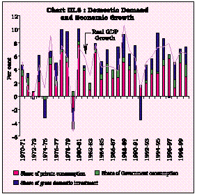
3.12 Decennial movements in domestic demand suggest that although private consumption has provided the underlying foundations of the growth process, it is investment which has enabled phases of acceleration and stability in periods of slowdown. The average relative contributions of government consumption increased in the 1980s but has remained stagnant in the 1990s (Table 3.1).
3.13 The relative contributions of the domestic demand components, except government consumption, have a pro-cyclical relationship with growth; periods of high growth are associated with higher growth of private consumption and domestic investment and lower growth in periods of downturn. Government consumption has a relatively small impact on the growth process. In the second half of the 1990s, especially since 1997-98, the deceleration in growth occurred on account of slowdown in private consumption and investment demand. Since 1997-98, the slowdown in private consumption has been substantial; the average contribution to growth has slipped to 3.0 percentage points during 1997-98 to 1999-2000 as compared with 4.5 percentage points during the period 1994-95 to 1996-97. In the case of investment demand, its contribution to growth has slipped to 2.0 percentage points which is lower than that of 2.9 percentage point during the high growth phase 1994-95 to 1996-97. On the contrary, government consumption has witnessed a counter-cyclical movement, indicating that discretionary fiscal stabilisers in the form of the Pay Commission awards have had a role in the limited context of holding up aggregate demand over the period of the downturn (Chart III.6).
|
3.14 A robust association between aggregate output and demand components emerges from the synchronous movement of their cyclical components. The correlation coefficient between the cyclical components (estimated by using pure cyclical components involving two stage filtering process to remove irregular components) of the sources of domestic demand between (private consumption, investment and government consumption) and the cyclical component of GDP is higher between private consumption and GDP than between investment and GDP, indicating the primacy of consumption in generating effective demand in the Indian economy. Government consumption has negative, albeit low and insignificant contemporaneous correlation with GDP, but has positive correlation after a lag. Thus, an increase in government consumption may depress aggregate demand initially and it will be some time before the intended demand boost takes effect. These differentials in associations have critical relevance for designi the timing and stance of counter-cyclical policies (Table 3.2).
Saving Behaviour
3.15 By developing country standards, India's saving rate continues to be fairly impressive; by the yardstick of some East-Asian economies, however, there is a considerable scope for improvement (Table 3.3).
3.16 The Indian savings experience has been marked by varied oscillations in the saving rate (Ray and Bose, 1997). After the initial phases of low saving, it reached a high during 1976-77 through 1979-80, reflecting, inter alia, the spurt in foreign remittances. Financial saving started assuming importance as a result of the financial deepening following bank nationalisation in 1969 (Table 3.4). After some lull during the first half of the 1980s reflecting deterioration in public savings as well as a step-up in the households' demand for consumer goods, the saving rate started recovering. The high growth phase of 1994-95 through 1996-97 is also accompanied by a high saving phase with the average saving rate touching a high of 24.4 per cent. The inflexion discernible in the growth rate in 1996-97 is also noticeable in the saving rates.
3.17 Several factors influencing saving behaviour such as income, interest rates and other variables have been explored in the empirical literature, using cross-section and time series data. Real GDP growth has generally been found to have exerted a positive effect on the savings rate (Fry, 1980; Giovannini, 1985). Contrary to conventional wisdom, some empirical studies have found a negative effect of real interest rate on savings (Giovannini, 1985). The transformation of domestic savings into additional income via accumulation of capital was found to be not only operative, but a significant factor in the growth of incomes in developing countries (Gersovitz, 1988). Saving is not just about accumulation but about smoothing consumption in the presence of liquidity constraints and uncertainties including those associated with the full stream of income on part of the individual households, typically in developing economies (Deaton, 1990). The issues pertaining to the effect of various determinants of savings are, thus, yet to be fully resolved.
3.18 In the Indian context, income is identified as an important variable in explaining savings rate, particularly for the household sector (Krishnaswamy, Krishnamurty and Sharma, 1987). Granger causality tests found evidence for growth influencing savings and not vice-versa. Other important determinants of savings behaviour are found to be the size of the working population, dependency ratio, financial deepening and taxation (Mulheisen, 1997). The studies on the effect of interest rate on savings in India have showed mixed results. A disaggregated analysis on the effect of the real interest rate on saving found a favourable impact of the rate of interest on some components of savings, i.e., currency and bank deposits (Pandit, 1985), and of the real interest rate on the savings rate of the households as well as for the economy as a whole (Krishnaswamy, Krishnamurty and Sharma, 1987), whereas other studies have yielded inconclusive results relating to the interest sensitivity of savings behaviour in India (Bhattacharya, 1985). Besides, spread of banking has been found to have a significant impact on savings (Krishnaswamy, Krishnamurty and Sharma, 1987).
(As percentage of GDP at current market prices) | |||||||||||
Period / Year | Households | Private | Public | Gross Domestic | |||||||
| | Financial | Physical | Total | Corporate | | Saving | |||||
1 | 2 | 3 | 4 | 5 | 6 | 7 | |||||
1976-77 to 1978-79 | 5.7 | 8.5 | 14.3 | 1.4 | 4.6 | 20.2 | |||||
1979-80 to 1984-85 | 6.1 | 7.1 | 13.3 | 1.6 | 3.8 | 18.7 | |||||
1995-86 to 1992-93 | 7.9 | 8.9 | 16.7 | 2.3 | 2.1 | 21.1 | |||||
1993-94 | 11.0 | 7.4 | 18.4 | 3.5 | 0.6 | 22.5 | |||||
1994-95 | 11.9 | 7.8 | 19.7 | 3.5 | 1.7 | 24.8 | |||||
1995-96 | 8.9 | 9.3 | 18.1 | 4.9 | 2.0 | 25.1 | |||||
1996-97 | 10.3 | 6.7 | 17.0 | 4.5 | 1.7 | 23.2 | |||||
1997-98 | 9.9 | 8.0 | 17.8 | 4.2 | 1.5 | 23.5 | |||||
1998-99 | 10.9 | 8.2 | 19.1 | 3.7 | -0.8 | 22.0 | |||||
1999-2000 | 10.5 | 9.2 | 19.8 | 3.7 | -1.2 | 22.3 | |||||
Source : Central Statistical Organisation. | |||||||||||
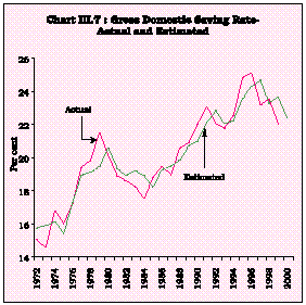
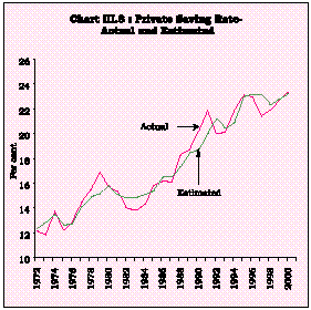
3.19 The savings behaviour in the Indian context is analysed for the period 1970-71 to 1999-2000 by estimating savings functions at the aggregate level, and also for private saving. The empirical estimates indicate that real per capita income and financial deepening have significant positive effects on the aggregate saving rate (gross domestic saving rate) and are its main determinants1; other things remaining the same, a one per cent increase each in income and intermediation ratio (secondary issues to primary issues ratio, as used in flow of funds accounts) would induce an increase in aggregate savings rate by 6.6 percentage points and 3.4 percentage points, respectively. The interest rate, i.e., real deposit rate, has a lesser but positive impact on gross savings rate; implying that as much as 12 percentage points change in the real interest rate is required to increase aggregate savings rate by one percentage point. The results indicate that the dynamic response of the private saving rate to per capita income (per capita disposable income is the relevant scale variable in studying private saving behaviour) works out to 7.8. The in-sample fits of the estimated equations for aggregate and private savings rates, are reported in Charts III.7 and III.8.
|
|
Investment Behaviour
3.20 The relationship between investment (i.e., capital formation) and output assumes special importance in the case of capital-deficient developing countries, especially in the reinvigoration of growth. Studies have typically shown that capital accumulation contributes up to 60-70 per cent of the growth in per capita output (IMF, 2000) and continues to be the primary engine of growth. In India, the deceleration in growth in the second half of the 1990s is associated with slowing rate of investment. It is in this context that a study of investment behaviour in India assumes importance.
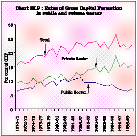
3.21 The rate of nominal gross capital formation (GCF) rose from 15.8 per cent in 1970-71 to 22.7 per cent in 1999-2000 undergoing two phases of deceleration, first in the early 1980s and again in the second half of the 1990s. The rate of capital formation has been rising in the private sector while in the public sector, it has been generally declining in the 1990s (Chart III.9). An analysis of the behaviour of GCF in terms of industry of origin in the 1990s indicates that the rate of capital formation in agriculture exhibited a slow decline from 2.0 per cent in 1992-93 to 1.7 per cent in 1998-99. The rate of capital formation in industry underwent a steep fall from 1995-96 onwards. There was a declining trend in the rate of capital formation in the services sector in the 1990s until 1999-2000. In all, a clear slowdown in the investment demand across the sectors was visible in 1990s, especially in the mid-1990s. This has been reflected in the downturn of growth.
|
3.22 In order to assess the investment behaviour of the economy in relation to growth, it is necessary to study investment behaviour in real terms. The real investment rate (adjusted for errors and omissions) moved up from an average of 21.8 per cent in the 1980s to 27.2 per cent in 1995-96 before decelerating to 26.0 per cent in 1999-2000 (Table 3.5).
3.23 The traditional view of investment in the context of growth cycles is in terms of its replacement cost. In a developing economy, apart from the rate of output growth, and replacement cost (or cost of capital), the rate of capacity utilisation, liquidity constraints faced by firms, and macroeconomic stability have been identified as major determinants of investment (Schimidt-Hebbel, Seren, and Solmano, 1996). An important issue in the study of investment in India is the relation between public and private investment, particularly in the context of the vacation of public investment in several areas to create space for private investment as part of the structural reforms in the 1990s. In India, the broad consensus favours a crowding-in relationship between public and private investment (Sundarajan and Thakur, 1980). The major determinants of corporate investment in India have been found to be credit availability and cost of capital (Athukorala and Sen, 1996).
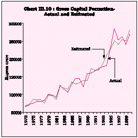
3.24 An econometric investigation has been undertaken to estimate the behaviour of aggregate GCF, as well as private investment in various constituent sectors by industry of origin, i.e., agriculture, manufacturing and services, over the period 1970-2000 in the conventional accelerator framework specifying lagged structures for output effects. Besides real GDP, important determinants of investment are postulated to be the real bank lending rate, and public investment in the services sector to capture possible 'crowding-in' effects2. The in-sample fits of the investment rates are presented in Chart III.10. Two findings emanate from the exercise. First, the aggregate investment is positively and significantly influenced by income, both contemporaneously and with a lag reflecting the operation of the acceleration principle, i.e., investment demand is induced by past output. Secondly, public investment in services favourably impacts private investment in manufacturing and services, corroborating the operation of a crowding-in phenomenon between appropriate types of public and private investment.
|
Nurturing Short-run Growth Impulses
3.25 In the tradition of growth models, investment simultaneously contributes to effective demand in the economy and augments the productive capacity, thus, providing the static Keynesian analysis with a dynamic perspective. In this section, the analysis hopes to provide pointers for the allocation of resources in support of reviving growth. For this purpose, working out investment multipliers and accelerators as well as multiplier-accelerator interaction becomes crucial for gauging the strength and duration of virtuous cycles of investment and output so as to direct the deployment of investible resources. The multiplier determines the initial injection of investment that is necessary to generate a desired increase in income. The accelerator measures the response of investment to changes in demand conditions. The multiplier and accelerator together capture the simultaneous interaction of investment and income (demand).
3.26 A simple econometric investigation of the real private final consumption expenditure in relation to real GDP at factor cost over the period 1970-71 through 1999-2000 yielded the marginal propensity to consume with respect to current income of about 0.60, implying a multiplier value of 2.5. Thus, a one per cent increase in, say, government spending or autonomous private investment would raise income by 2.5 per cent (Table 3.6).3
Variable | Multiplier |
1 | 2 |
Private Final Consumption | 2.5 |
Government Final Consumption | 1.2 |
Overall Consumption | 3.9 |
3.27 Increases in government spending and private investment could induce greater utilisation of the economy's productive capacity which, in turn, may increase income levels more than implied by the static multiplier. The inter-temporal effects of the initial stimulus to aggregate demand feeds into the income stream through a series of complex interactions between consumption behaviour and investment spending to produce cumulative expansions in income which have been described in the literature as 'super multiplier' (Rangarajan and Dholakia,1999). Illustratively, an initial injection of spending in the form of government expenditure generates an increase in income via the conventional static multiplier. The increased income can induce changes in consumption demand as well as expansion in the demand for productive capacity (i.e., investment demand), both private and public. Thus, fiscal policy intervention in the form of expenditure on consumption and investment is now determined within the dynamics of the income-expenditure propagation process (super multiplier) rather than exogeneous to it. This brings in the key issue of the sustainability of the envisaged growth path and the role of fiscal policy. Specifically, there emerges a critical limit up to which 'pump-priming' can be undertaken without rendering the growth process unstable.
From the empirical exercise conducted here, the upper limit for counter cyclical deployment of government consumption can be worked out as close to 15-17 per cent of GDP. Given that the current ratio of government consumption to GDP is at 14 per cent, there appears to be very little leeway for any further pump-priming through government consumption. Beyond the limit, pump-priming would impart instability to the growth process.
3.28 The accelerator theory of investment focuses directly on the motivation for and purpose of investment expenditures to maintain and/or increase productive capacity so as to meet the future demand for the commodities produced by the firms. Specifically, the acceleration principle relates the desired investment demand to the changes in output in the previous period. The interaction of the multiplier along with the accelerator generates a dynamic income path in response to a shock to an autonomous component of demand. The accelerators, as derived from the earlier specifications of both aggregate investment as well as sectoral investments in the private sector are presented in Table 3.7. Two features follow from the estimates. First, the estimated values of marginal propensity to consume and accelerator generated stability of the income path. Thus, the multiplier and accelerator interaction in the Indian economy would generate stable and converging cycles, thereby making room for counter cyclical policies. Secondly, sectoral accelerators show that greater investment needs to be directed towards manufacturing so as to revitalise growth. Illustratively, assuming a target growth path of 8 per cent, the multiplier-accelerator interactions suggest that a unit increase in government spending yields highest dynamic income multiplier effect for manufacturing at 4.73, followed by services at 4.12 and agriculture at 3.89.
Type of Investment | Accelerator |
1 | 2 |
Private Investment in Agriculture | 0.04 |
Private Investment in Manufacturing | 0.61 |
Private Investment in Services | 0.21 |
Net External Demand
3.29 External demand has played a relatively small role in influencing the course of the business cycles in India, given the low degree of openness. The empirical evidence, however, suggests that trade flows provide conduits for global integration which are stronger and larger than what any conventional measure of net exports would suggest. This is increasingly evident in India with the pattern of exports and industrial production exhibiting certain degree of co-movement with the global business cycle (Chart III.11).
|
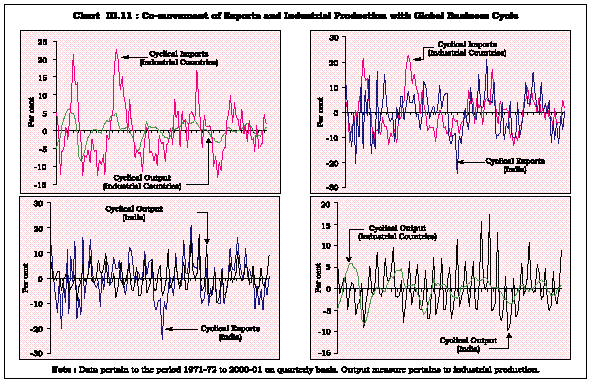
3.30 'Granger' causality provides a simple test of the direction and intensity of causal relationships. Empirical analysis indicates that cyclical output in industrial countries 'Granger' causes imports of these countries unidirectionally, implying that cycles in the advanced economies have significant effects on their import demand. The causality between cyclical imports of advanced countries and India's exports is significant and strongly bi-directional. Cyclical output of advanced countries has unidirectional causal effects on cyclical output in India (Table 3.8).
3.31 In the 1990s, however, traditional measures of net external demand have lost operational relevance especially in view of the dominance of financing flows in the balance of payments. Moreover, the net capital flows are no longer viewed in a passive financing role. Considerations of reserve adequacy have ensured that the movements of capital are no longer dictated by current account outcomes (IMF, 1997). Growth in the volume of cross-border capital flows, however, clearly dominated every other form of cross-border transaction during the 1990s. Capital flows have emerged as the predominant engine of globalisation and growth convergence across nations. It is in this context that Chapter VI of the Report devotes itself to an examination of the obverse of net exports, i.e., capital flows.
II. STRUCTURAL CONSTRAINTS IN INDIAN AGRICULTURE
3.32 There has been a growing concern in recent years about the constraints on growth on account of the high variability of agricultural output on one hand, and the deceleration of the agricultural output in the 1990s in relation to the high growth phase of the 1980s, on the other. There has been a near stagnation in yield levels and limits seem to have been reached in further expanding the area under cultivation. Equally important is a growing anxiety that the process of reforms has by-passed the agricultural sector (Reddy, 2001). Accordingly, extending reforms to the farm sector and achieving robust growth in the agriculture holds the key to reversing the industrial slowdown4. The search for realisation of the full growth potential of the agricultural sector has motivated extensive research in India. The critical constraining factors cited in these studies are declining public sector capital formation in agriculture (Gulati and Bathla, 2001); the low agricultural supply response to price incentives in the form of higher procurement prices (Balakrishnan, 2000); excessive dependence on input subsidies-particularly fertiliser, power, water and credit (GoI, 2000a); weak rural credit institutions and declining effectiveness of formal credit arrangements for agriculture (Vyas, 2001); the implicit indirect tax on agriculture as measured by the aggregate measure of support to agriculture (Hanumantha Rao, 2001); and overpopulation in agriculture and the resultant increase in the number of small sized farms which are economically unviable. Besides these studies, various impediments to agricultural progress have been identified by official assessments (GoI, 2000a, RBI, 2001): continued rain dependency of agriculture; poor adoption of new technology and its unsuitability to the varied soil and moisture conditions; inappropriate rural infrastructure; and weak marketing structure; and archaic land holding and tenancy laws. Accordingly, a growing consensus is emerging in India for prioritising policies for the modernisation of Indian agriculture (Rao and Jeromi, 2000).
3.33 International experience suggests that high agricultural growth and productivity generally precedes or accompanies industrial growth in most successful cases of economic development. Agriculture's contribution to the overall growth process of an economy has traditionally been in the form of: (a) supplying the surplus labour to the non-farm sector, (b) making available wage-goods at reasonable prices to sustain the labour force in the non-farm sector, (c) generating savings for investment in the non-farm sector, (d) earning foreign exchange through exports to finance critical imports, and (e) creating demand for the output produced in the non-farm sector. The changing mix and the continuous interaction between the farm and the non-farm sector assumes critical importance in the growth process as it offers opportunities for internalising the synergetic growth impulses even in a period of decline in the share of agriculture in real GDP.
3.34 In India, agriculture occupies a special position in the development process. It continues to provide a ratchet to the overall GDP growth, in view of the continued dependence of up to two-thirds of the population on agriculture. In this section, an attempt is made to identify the constraints to higher agricultural growth. Drawing from an overview of the changing pattern of growth and productivity of Indian agriculture over the past three decades, an analysis of the major determinants of agricultural growth in India is undertaken to identify bottlenecks choking the growth prospects of Indian agriculture and to suggest proximate solutions.
Changing Patterns of Growth and Productivity
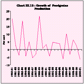
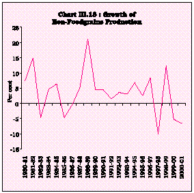
3.35 Agricultural output growth registered a sharp increase in the immediate post-green revolution phase largely due to a growth in yields; however, the growth pattern has not been uniform with a tendency towards deceleration in the 1990s (Table 3.9 and Charts III.12 and III.13).
|
|
3.36 The yield pattern in case of both foodgrains and non-foodgrains indicates that highest growth in yield levels occurred during the 1980s. Much of the growth in agricultural production in India is yield-driven as the growth in area is marginal; however, Indian agriculture suffers from lower yield levels vis-à-vis major agricultural producers in the world, despite India being one of the largest producers of most of the major crops (Table 3.10). The yield of 6,059 kg per hectare attained in China during 1998 in the production of paddy was more than double that of 2,890 kg per hectare in India. Similarly, wheat yield in China stood at 3,667 kg per hectare in 1998 in comparison with 2,578 kg per hectare in India.
The Role of Technology in Indian Agriculture
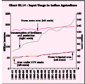
3.37 One of the main reasons for the low levels of yield attained in India is the unsatisfactory spread of new technological practices, including cultivation of High Yielding Varieties (HYV) of seeds. The adoption of new technology, mainly the cultivation of HYV seeds requires intensive use of fertilisers and pesticides under adequate and often assured water supply. The use of HYV seeds entails a higher yield risk (as measured by variance in yield) as compared with the traditional seed varieties, in the absence of proper irrigation facilities (Ganesh Kumar, 1999; Saha, 2001). The lower spread of new technological practices to a wide variety of crops other than wheat and rice as also across regions could be attributed to the higher yield risk associated with the cultivation of HYV seeds, caused by inadequate spread of irrigation facilities. There is considerable co-movement between the area under HYV seeds and area under irrigation, probably on account of reduction in yield risk due to irrigation facilities (Chart III.14).
|
3.38 It is mainly paddy and wheat, which are cultivated under the HYV seeds, while the areas under HYV seeds for other cereal crops are very low and vary across different States of the country. Low growth experienced during the past two decades in the production of coarse cereals (0.5 per cent) and pulses (0.8 per cent) in comparison to rice (2.8 per cent) and wheat (4.0 per cent) is on account of lower adoption of HYV seeds or non-availability of appropriate seeds (apart from the usual dry-land farming accorded to these crops), given the diverse soil and moisture profiles of different parts of the country. The pattern of adoption of HYV seeds across various states has accordingly been disparate (Table 3.11).
3.39 One significant factor limiting the adoption of HYV seeds is the generally low level of irrigation cover for most of the crops as compared with rice and wheat. Nearly 64 per cent of the total cultivated area in the country is rain-fed. In fact, as compared with 79.1 per cent of the total geographical area as drought prone, the irrigation coverage of 38.2 per cent is quite unfavourable. The Ninth Plan document placed the irrigation potential at 139.89 million hectares. With this irrigation potential, the cropping intensity coefficient can be raised up to 149.0 as against the current level of 134.20.
It has been found that the States of Rajasthan, Gujarat and Jammu and Kashmir have a higher probability (in excess of 20 per cent) of the incidence of drought in any given year. Moreover, agriculturally important States such as Andhra Pradesh, Uttar Pradesh, Haryana and Punjab have been found to have more than 10 per cent probability of the incidence of drought in any year (Sinha Ray and Shewale, 2001). Of these, only Punjab has a good irrigation cover, while Haryana has a moderately good irrigation coverage (Table 3.12). Wheat and rice among foodgrains and sugarcane among non-foodgrains enjoy the maximum irrigation coverage across all States. Even in the States with lesser irrigation coverage, such as Karnataka, Madhya Pradesh, Kerala, etc., the irrigation cover for rice and wheat is much higher in comparison with other crops. Thus, in India irrigated area generally tends to be used for the growing of rice and wheat, while the other crops are grown mostly in rain-fed and unirrigated conditions.
3.40 In such a scenario, the technological development in terms of the adoption of HYV seeds is mostly limited to the cultivation of rice and wheat on account of higher yield risk imparted by these seeds. It is pertinent to note in this connection that the foodgrains production in 1999-2000 was at a record high of 208.9 million tonnes despite acute drought conditions in the central stretch of India, mainly on account of record production of rice and wheat. Most of the other crops - mainly oilseeds - suffered significant fall in production in that year. This could be indicative of the disproportionate adoption of technology and irrigation benefits, underscoring the need for spreading the irrigation benefits to all crops.
3.41 Another important factor affecting the dissemination of modern technology in general and HYV seed technology in particular is the small size of average farms in India. It has been argued that the small size of land holdings limits the adoption of new technology due to reasons other than the scale of operation. Share-cropping, which is generally undertaken by the small and marginal farmers, limits the scope for adoption of new technology as the farmer has to pay a fraction of (generally around half) the production to the land-owner, while the whole cost of adoption of the green revolution inputs such as HYV seeds and fertilisers will have to be borne by the tenant. In such an arrangement, it is imperative that the gains in marginal product due to adoption of these inputs should at least be twice that of the investment for the farmer to break even. Such dramatic increases in production are difficult to come by in the absence of other infrastructural facilities and hence, the scope for adoption of green revolution inputs by the share-cropper is clearly undermined.
3.42 The per hectare consumption of fertilisers and pesticides is quite low in India in comparison with international standards and there is a lot of scope for improvement in this sphere. For instance, the per hectare consumption of fertilisers in India at 88.6 kg was much lower than 256.6 kg and 110.4 kg in China and USA, respectively, in 1997-98. The growth in the consumption of fertilisers during the past two decades has also quite varied across different States (Table 3.13). Another factor that is responsible for lower productivity of Indian agriculture is the skewed distribution of N:P:K (Nitrogen : Phosphorus : Potassium) fertiliser mix. Currently, the N:P:K ratio stands at 6.9:2.9:1.0, which is quite skewed in comparison to the optimal mix of 4:2:1. The skewed consumption of fertiliser accentuates the risk of salination and leaching of soil, thus hampering the long-term productivity of the land. This skewed fertiliser consumption pattern is the result of highsubsidies extended to the urea producers.
Table 3.13 : State-wise Trend Growth Rates of Area Under HYV Seeds and per Hectare Fertiliser Consumption |
(per cent) | |||||||||||
State | Area under | Per Hectare | |||||||||
HYV seeds | Fertiliser | ||||||||||
| | | | Consumption | ||||||||
1 | | 2 | 3 | ||||||||
Andhra Pradesh | 1.15 | 6.21 | |||||||||
Assam | 2.74 | 10.63 | |||||||||
Bihar | 2.09 | 8.03 | |||||||||
Gujarat | 0.68 | 5.18 | |||||||||
Haryana | 1.09 | 6.80 | |||||||||
Himachal Pradesh | 2.12 | 3.97 | |||||||||
Jammu & Kashmir | 2.16 | 5.02 | |||||||||
Karnataka | 5.68 | 5.27 | |||||||||
Kerala | -4.83 | 3.51 | |||||||||
Maharashtra | 3.63 | 7.10 | |||||||||
Madhya Pradesh | 5.99 | 8.36 | |||||||||
Orissa | 6.14 | 7.40 | |||||||||
Punjab | 1.77 | 1.81 | |||||||||
Rajasthan | 2.72 | 9.26 | |||||||||
Tamil Nadu | 1.62 | 3.54 | |||||||||
Uttar Pradesh | 3.40 | 4.53 | |||||||||
West Bengal | 5.50 | 6.62 | |||||||||
All-India | 3.10 | 5.29 | |||||||||
Notes : | 1) The growth rates for area under HYV seeds pertain to 1980-81 to 1996-97, and those for per hectare consumption of fertilisers relate to 1980-81 to 1999-2000. |
2) Trend Rates are based on semi-logarithmic function. |

ಈ ಪುಟವನ್ನು ಹಂಚಿಕೊಳ್ಳಿ:


ಭಾರತೀಯ ರಿಸರ್ವ್ ಬ್ಯಾಂಕ್ ಮೊಬೈಲ್ ಅಪ್ಲಿಕೇಶನ್ ಅನ್ನು ಇನ್ಸ್ಟಾಲ್ ಮಾಡಿ ಮತ್ತು ಇತ್ತೀಚಿನ ಸುದ್ದಿಗಳಿಗೆ ತ್ವರಿತ ಅಕ್ಸೆಸ್ ಪಡೆಯಿರಿ!
ನಮ್ಮ ಅಪ್ಲಿಕೇಶನ್ ಅನ್ನು ಸ್ಥಾಪಿಸಲು QR ಕೋಡ್ ಅನ್ನು ಸ್ಕ್ಯಾನ್ ಮಾಡಿ


ಪೇಜ್ ಕೊನೆಯದಾಗಿ ಅಪ್ಡೇಟ್ ಆದ ದಿನಾಂಕ:


