 IST,
IST,


RBI WPS (DEPR): 04/2024: Assessing the Impact of Macroprudential Policies on Housing Credit Dynamics: Evidence from India
|
RBI Working Paper Series No. 04 Assessing the Impact of Macroprudential Policies on Housing Credit Dynamics: Evidence from India Amar Nath Yadav, Vivek Kumar, Alok Kumar Chakrawal and Jyoti Kumari1 Abstract This paper evaluates the efficacy of macroprudential (MaP) policy in modulating bank credit to the housing sector and its impact on the asset quality of banks in the Indian context. The empirical analysis suggests that a tightening of MaP policy is effective in controlling bank credit to the housing sector. Tightening policies appear to have a greater impact on credit growth than easing policies. Furthermore, a tighter MaP policy complemented with a tighter monetary policy helps in reducing non-performing assets in the housing sector. JEL Classification: C23, E58, G21, G28 Keywords: Macroprudential policies, housing credit, credit risk Introduction The major objective of macroprudential (MaP) policies is to strengthen the banking and the financial system through pre-emptive regulatory measures (G30, 2009; IMF, 2009; Brunnermeier et al., 2009; and TdLG, 2009). These policies aim at preventing or mitigating the consequences of busts in the credit cycles by utilising the buffers built during booms. Their countercyclical nature assists in dampening credit cycles – these can help to contain excessive credit growth during boom times and support credit growth during downswings in economic activity. Generally, they are intended to complement microprudential regulations as well as conventional macroeconomic management instruments, notably monetary and fiscal policies. According to Adrian and Shin (2010), the increasing interconnectedness of financial institutions and the excessive growth of assets held by them can also cause systemic risks. Therefore, effective MaP policies can contribute to the stability of the financial system. Since the global financial crisis of 2008, the G20 has supported the use of MaP policies as part of its international regulatory reform agenda. The increasing use of the MaP policies, however, has given rise to a pertinent question about their efficacy. Recent studies on intermediate indicators of systemic risks have provided some evidence about their effectiveness with regard to credit growth and asset prices (Lim et al., 2011; Cerutti et al., 2015; Kuttner and Shim, 2016; Zhang and Zoli, 2014; Akinci and Olmstead-Rumsey, 2018). However, the evidence is still quite scattered for both advanced and emerging economies. Furthermore, a majority of the empirical evidence till now, particularly in the Asia-Pacific region, is from commercial databases or at the systemic level and not at the bank level. India too has a long history of utilising MaP policies such as Loan-to-Value (LTV) ratios, risk weights, and sector-specific policies. There are studies assessing the efficacy of these policies at the aggregate bank credit (Verma, 2018) and sector-specific levels (Saraf and Chavan, 2023). However, the existing studies have not adequately captured the issue of whether and how far MaP policies have helped in controlling credit risk. In this paper, we evaluate the impact of MaP policies exclusively on the housing sector, which is one of the largest segments of retail credit in India and assess their impact on housing credit growth and non-performing assets (NPA) using bank-level data. Additionally, our paper explores how the stance of monetary policy, the economic cycle, and the financial cycle can affect the impact of MaP. The empirical strategy used in this paper is as proposed by Cantu et al. (2019). The structure of the paper is as follows. Section II provides a review of MaP policies that have been used in the past by different countries and their effectiveness. Section III highlights the MaP policy instruments adopted in India over time. The data and methodologies employed are discussed in Section IV. Section V outlines the results and observations. Finally, we draw conclusions and provide implications for potential policies in Section VI. II. Review of Macroprudential Policy Measures and Their Impact A wide variety of MaP tools are included in the MaP policy toolkit. Both advanced economies (AEs) and emerging market economies (EMEs) utilise various mechanisms to mitigate the impact of systemic risk and minimise the negative effects of externalities on the financial sector. While there has been a greater receptivity to MaP policies in AEs, particularly after the global financial crisis (GFC), EMEs have had a longer experience with them given the greater vulnerability of the financial systems in these economies to adverse shocks. Even though a major part of Asia was not directly affected during the GFC, the Asian regulators gave a focused attention to MaP policies, particularly the LTV ratio. Also, the Asian financial crisis of 1997 provided an opportunity to these regulators to experiment with these instruments over a longer period. The LTV policies have been shown to be effective in some Asian countries. Wong et al. (2011) examined the effects of LTV on mortgage delinquency ratios and other measures of market activity, such as housing prices and household debt. Mortgage delinquency ratios were significantly reduced after the introduction of LTVs. An analysis of a panel data set of 13 Asian economies (including India) and 33 other AEs and EMEs by Zhang and Zoli (2014) reveals that MaP tools contributed to reducing the procyclicality of credit in Asia - housing-related tools, including LTV ratios, debt-to-income ratios (DTI), risk weights, and loan loss provisions for mortgage loans, had a significant impact on bank credit, while changes in reserve requirements and capital regulations had a limited impact. The study by Kuttner and Shim (2012), which examined the effectiveness of housing-related MaP policies in 57 AEs and EMEs between 1980 and 2011, found that these measures were successful in restraining the expansion of housing credit and maintaining stability in housing prices. There was a noteworthy correlation between the prudential variables associated with housing sector credit and the LTV ratio. However, no significant correlations were observed between the LTV ratio and the exposure limits imposed on banks in relation to the housing and property sectors. Claessens et al. (2014) utilised bank-level data from 48 AEs and EMEs for the period 2000-2010 and found that MaP instruments were more effective at maintaining financial intermediation in upswings than during contractions. Similarly, Cerutti et al. (2015) examined 119 countries over the period 2000 to 2013, and upheld the efficacy of MaP policies. Tressel and Zhang (2016), focusing on the Euro area, examined the impact of instruments targeting the cost of bank capital on mortgage credit growth. They utilised the Euro-system Bank Lending Survey and found that these instruments had a significant effect in slowing down mortgage credit growth. Additionally, the study highlighted the effectiveness of LTV limits, particularly when monetary policy was eased. In Erdem et al. (2017), the data from 30 EMEs, including India, covering the period from 2000 to 2013, was analysed to judge the efficacy of MaP policies in regulating the growth of domestic credit. While underscoring the effectiveness of MaP policies, the study highlighted the challenges of preventing leakages and maintaining the effectiveness of MaP instruments during a global liquidity crisis. Verma (2018) investigated the efficacy of MaP policy in India by utilising annual data from 1999-00 to 2016-17. Using a panel vector auto-regression (VAR) framework based on bank groups, the study found that a tightening of MaP measures had an adverse effect on credit growth with a one-year lag. The findings were similar for sectors such as housing, commercial real estate and consumer loan portfolios. However, their usefulness in promoting credit growth during periods of economic downturn proved to be limited. Sanjiv et al. (2022) investigated the efficacy of MaP policy on bank credit, housing credit, and housing prices in India using a structural vector autoregression (SVAR) on monthly data from 2004-2020. The study demonstrated that MaP policy successfully controlled bank credit, housing credit, and housing price inflation. Moreover, it showed evidence of the asymmetric effect of MaP policy, wherein tightening action had a considerable impact on bank credit and housing prices and easing action largely influenced housing credit. Saraf and Chavan (2023) analysed the efficiency of the MaP policy in managing systemic risk in India using bank-level supervisory data for five major sectors, including the housing sector. They found that the dynamic risk weights and provisioning as tools of MaP were not statistically significant for controlling loan growth in the retail housing sector while the LTV ratios were found to be effective. Many of these studies have either used aggregated or annual data in their analysis. Aggregation not only leads to a loss of information but also limits inferences about the behaviour of individual financial institutions. Further, distinguishing between long-term and short-term effects of the policies may become difficult with annual data. To address these difficulties, we employ bank-level quarterly data in this paper. Also, the existing studies have not assessed the effect of the MaP policy on credit quality, as has been attempted by us. India has a strong track record in implementing countercyclical MaP policies, with a sector-specific focus. Key sectors targeted under this approach include capital market exposure, commercial real estate, residential housing, other retail sectors, and non-bank financial companies. An early recourse to the MaP policy was intended to counter the impact of interest rate fluctuations on marked-to-market profits of banks in the early-2000s. During this period, banks’ profits were boosted from a fall in interest rates. To safeguard their balance sheets and prepare for the monetary cycle reversal and higher interest rates, the Reserve Bank of India (RBI) directed banks to establish an investment fluctuation reserve (IFR). The IFR required banks to transfer a portion of their investment gains over a five-year period, aiming to reach at least 5 per cent of their investment portfolio. In 2004, during an expansionary phase of the economy, the MaP measures included pre-emptive countercyclical provisioning and the application of differentiated risk weights for the sectors more sensitive to the economic fluctuations. The goal was to prevent excessive lending and risk-taking during economic booms, which could create vulnerabilities and potentially lead to financial crises. To address inter-connectedness in the financial system, the RBI introduced a framework in 2004 for enhanced monitoring and supervision of large and systemically important financial institutions or groups, commonly known as financial conglomerates. This framework aimed to identify and mitigate risks arising from the interconnections between these institutions, ensuring that their failure did not pose a significant risk to financial stability. Furthermore, the RBI implemented a capital conservation buffer under the Basel III framework in a phased manner with the last tranche of 0.625 per cent active from October 1, 2021. The framework on Countercyclical Capital Buffer (CCyB) was also put in place by RBI in February 2015 to be activated when the circumstances warranted. The CCyB requires banks to maintain additional capital during periods of excessive credit growth, creating a buffer to absorb potential losses. The RBI introduced additional capital requirements for domestic systemically important banks (D-SIBs). D-SIBs are considered to be of systemic importance due to their size, interconnectedness, complexity, and overall significance. The additional capital requirements for D-SIBs aim to enhance their resilience and reduce the likelihood of their failure and its potential impact on the financial system. III.1. Housing Credit Measures for Banks The RBI has deployed a variety of MaP measures for the housing sector, based on the evolving economic and financial cycles, and monetary policy settings. These include LTV ratios according to the size of the loan and category of loan (priority sector loan or non-priority sector loan), risk weights and standard provisioning. Changes in risk weights affect the capital ratio of the banks, while provisioning affects their profits. III.2. Time-Varying Risk Weights and Provisioning Norms India witnessed a disproportionately higher growth in housing credit during the period of high growth and robust capital inflows from 2004 to 2008 (Chart 1). This trend was observed alongside increasing real estate prices. To address the potential risks associated with this credit expansion, the risk weight on retail housing credit was raised from 50 per cent to 75 per cent in December 2004. Furthermore, the RBI made changes to the risk weights on housing credit based on loan size and LTV ratio. The risk weight on smaller-sized housing loans, considered as priority sector loans, was reduced from 75 per cent to 50 per cent while for larger loans and those with an LTV2 ratio exceeding 75 per cent, the risk weight was increased to 100 per cent. 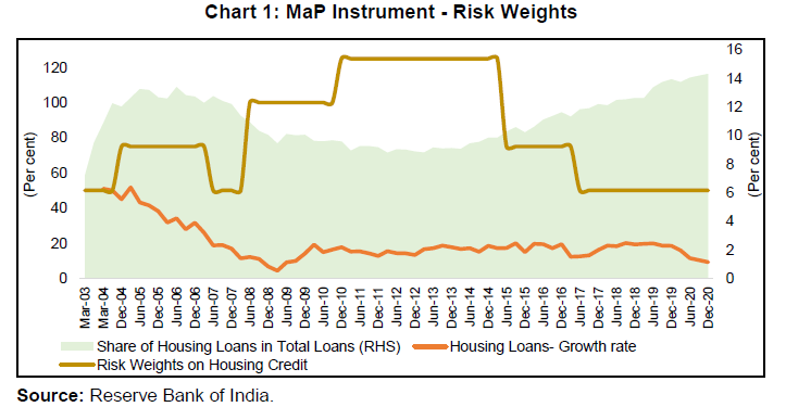 In 2010, the RBI increased the standard asset provisioning on outstanding housing credit from 0.40 per cent to 2.00 per cent which was subsequently reduced starting from 2013 onwards (Chart 2). The RBI also implemented changes in LTV policy in November 2015 and October 2016 (Annex: Table A1). 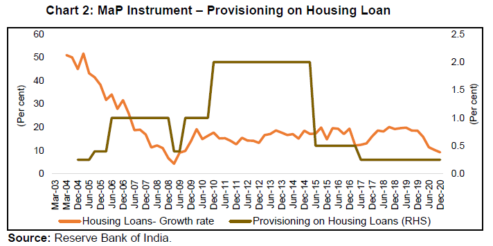 In sum, as highlighted by the Financial Sector Assessment Programme (FSAP-2012) of the IMF, India has had a long history of using MaP instruments to counter credit cycles and strengthen the banking system. The LTV policy of RBI has enhanced system resilience (Lu, 2019); this makes the Indian MaP policy relating to the housing sector an important case for study, as attempted in this paper. IV. Data and the Econometric Model The paper uses bank-level quarterly data of 51 major banks3, covering the period from Q1:2002 to Q3:2020. This paper examines the impact of MaP policy on housing credit growth and its NPAs, controlling for individual bank characteristics, such as asset size, liquidity situation, capital ratio, and funding ratio. Furthermore, we consider the impact of these policy actions across the different periods of the business and financial cycles, and the monetary policy cycle. The housing credit growth and NPA ratio are used as response variables. The four bank-specific control variables as described in the cross-country analysis framework of Cantu et al. (2019) are used: size (log of total assets), capital ratio (ratio of Tier-1 capital to total assets), funding ratio (deposits share in total liabilities), and liquidity ratio (liquid assets in relation to total assets). These controls are chosen to account for factors at the bank level that can influence strategic lending decisions. The macroeconomic controls are nominal GDP, repo rate, and other relevant variables4. To assess the stage of the financial cycle, credit-to-GDP gap was used. A full list of variables is provided in Annex Table A2. We also include dummies which represent the intent of MaP policy changes and the adjustments related to these changes, and baseline capital requirements. First, we examine the overall impact of MaP tools on housing credit growth and bank risk. To do so, we have used a dummy, which takes a value of +1 when the RBI signals a tightening of the policy, i.e., increase in LTV ratio or risk weight or provisioning in the quarter. It takes the value of 0 when there are no such policy adjustments, and -1 when the policy is eased or indicated to ease. As a second step, we introduce two separate dummies, one for tightening policy actions and the other for easing policy actions, to evaluate the differentiated effects of tightening and easing policy actions. We employ an indicator variable approach because of the difficulty of measuring the intensity of instruments. Furthermore, LTV was fixed according to loan size and amount, thus, constructing a cumulative index is difficult. Consequently, we utilise separate dummies to split MaP policy changes into easing and tightening cases to assess the asymmetric effects of each MaP tool. To address the merger/ consolidation of banks, we adjust our dependent variable after the merger. For other bank controls, no such adjustment was necessary, as no outliers were detected. The problem of endogeneity is one of the challenges that the literature speaks about when discussing the effects of MaP policy instruments. For the purpose of overcoming endogeneity, the system generalised method of moments (GMM) estimator, pioneered by Arellano and Bond (1991) is preferred due to its superior consistency and efficiency. It incorporates both the level equation and the difference equation, allowing for a more robust estimation of the model. The lag variables (up to lag 4) have been used as instruments. IV.1. Impact of MaP Policy on Housing Credit Growth To begin, the panel methodology is used to assess the impact of changes in MaP policy instruments on credit growth. The baseline regression model is defined as follows: 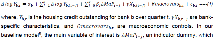  IV.2. Impact of MaP Policy on Different Types of Banks According to the literature on the bank lending channel, which discriminates between the supply of loan and the demand for loan movements based on cross-sectional differences between banks, different banks are able to buffer the impact of the policy on their loan portfolios differently. Small banks, which may encounter significant informational friction in financial markets, may have to pay higher interest rates to attract non-secured deposits if rules are tightened. Relatively illiquid banks could also be more affected by a tightening of policy if they face difficulties in reducing their holdings of securities. Thus, we propose the following amendments to our baseline specification: 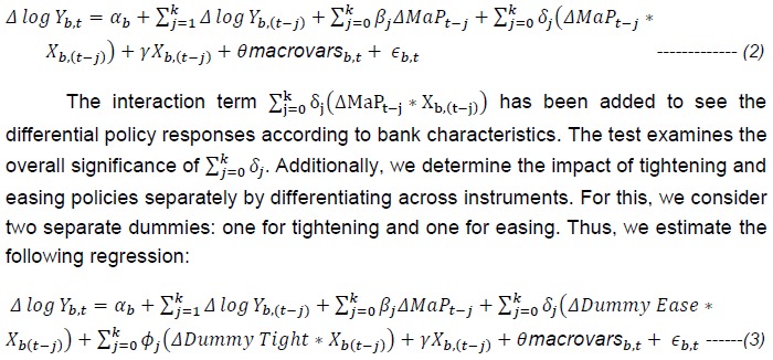 IV.3. Response of MaP Policy over Different Monetary Policy Conditions The favourable conditions for financing could have a positive impact on the demand for housing credit. Conversely, a more restrictive monetary policy could result in a decline in housing credit growth due to increased costs of funding for banks. In order to examine the effectiveness of MaP policy instruments under different monetary policy settings, the following equation is estimated (Bruno et al., 2017): 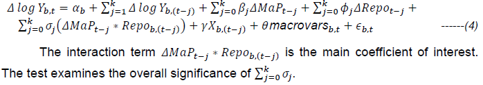 IV.4. Response of MaP Policy over the Business or Financial Cycle The paper also examines the differential effects of various phases of the business cycle and the financial cycle on MaP policy. The aim is to investigate as to whether the impact of MaP policy is amplified during periods of high GDP growth or conversely affected during periods of low growth. As a baseline specification for the business cycles, we estimate following equation: 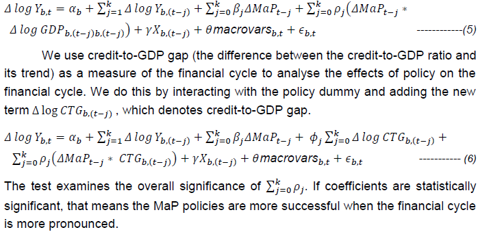 IV.5. Impact of MaP Policy on Non-Performing Assets To investigate the impact of MaP policy on banks' NPAs, our baseline specification is as follows: 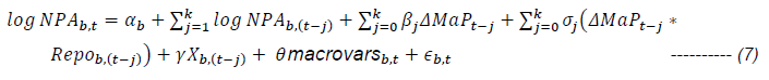 Here, the NPA is a ratio of gross non-performing housing credit to total housing credit. Since NPAs persist over time, lagged values of the NPA have been included as an explanatory variable. To determine whether there are any interactions between MaP policy and monetary policy, interaction terms have been included. Asset quality can also be impacted by variations in MaP policy, and therefore, it would be interesting to know the policy impact of easing and tightening instruments individually. To capture the separate effects of each instrument, our specification is as follows:  In the above equation, we also include the interaction for tightening and easing policy changes. The regression estimates for the models are reported in Tables 1-7. The tables are to be read as follows: in our baseline specification (no interaction term), the overall significance of the policy impact has been presented along with controls while the second column (with interaction term) presents the interaction effect. The policy impact is presented with one quarter lag for the short-term policy impact, while the sum of contemporaneous and four lags is presented separately for the overall size of the policy effect. V.1. Impact of MaP Policy on Housing Credit Growth The results of our baseline model show that the MaP policy can restrain the housing credit growth on an average, and the effect is statistically significant for two quarters (Table 1). The impact of bank controls interacted with MaP policy variable was not statistically significant except for the liquidity ratio and deposit ratio. The results also indicated that higher capital ratios boost housing credit growth, while the liquid assets ratio6 had a negative relationship with the housing credit growth. V.2. Impact of MaP Tightening and Easing Policy on Housing Credit Growth We employed two dummy variables to assess the impact of tightening and easing policies on housing credit growth independently. The dummy associated with tightening policies is negative and statistically significant for up to two quarters. When bank-specific interaction variables were included, the effect was lower. For easing MaP policy, the coefficient was negative and statistically significant, implying an increase in credit growth. However, tightening had a stronger impact than easing (Table 2). V.3. Response of MaP Policy over Different Monetary Policy Conditions The repo rate and the growth of housing credit were negatively correlated and statistically significant as shown in Table 3. The coefficient of the interaction term of MaP policy with repo rate was positive and statistically significant, indicating that when both MaP and monetary policies moved in the same direction, they had a stronger impact on housing credit growth. V.4. Response of MaP policy over Business Cycle and Financial Cycle The MaP measures were found to be more effective during high growth phase, as indicated by the interaction term (Table 4). The impact of MaP policy on housing credit growth during various phases of the financial cycle did not vary significantly (Table 5). V.5. Impact of MaP Policy on NPAs As per our baseline specification, the MaP policy coefficient did not have a statistically significant impact on the NPA ratio in the housing sector. However, when we included the interaction term with the repo rate, the MaP coefficient was positive and statistically significant (Table 6). We did not find any noteworthy influence of the bank-specific characteristics on the NPA ratio. We also considered two separate dummies for tight and easy MaP policies (Table 7). We observed that a tighter MaP policy decreased the NPA ratio, while an easy policy did not have a significant effect. Since any tightening applies to the entire loan portfolio including new loans, the NPA ratio may reduce because of a rebalancing of the risk weight and provisioning. This paper evaluated the effectiveness of MaP policy instruments in influencing housing credit growth and credit quality in India using bank-level quarterly data. The empirical analysis indicates that the MaP policies were effective in influencing housing credit growth. Banks’ capital adequacy had a positive impact on housing credit growth. MaP policies and monetary policies were more effective when used in tandem. MaP policies were not weakened by business cycle booms. While MaP policy alone did not seem to affect housing sector NPAs, tighter MaP and monetary policies in conjunction could help to reduce the NPA ratio in the housing sector. Stress tests, which are deployed for identifying potential vulnerabilities in the financial system, can guide the calibration of MaP policies within the regulatory toolkit. 1 Amar Nath Yadav (anyadav@rbi.org.in) is Assistant Adviser; Vivek Kumar is Director and Jyoti Kumari is Manager in the Department of Statistics and Information Management (DSIM), Reserve Bank of India, Mumbai. Alok Kumar Chakrawal is Vice-Chancellor of Guru Ghasidas Vishwavidyalaya, Chhattisgarh. The useful comments and suggestions received from Avdhesh Kumar Shukla, Sanjeev Kumar Gupta, Rajesh Kavediya, Arpita Agarwal, Priyanka Upreti and an anonymous external reviewer are gratefully acknowledged. We thank A. R. Joshi, Principal Adviser, DSIM for his valuable guidance and support. The views and opinions expressed in this paper are those of the authors and not necessarily represent those of the institutions to which they belong. 2 The RBI introduced the LTV cap as a function of loan size for the first time in India on May 14, 2008. 3 The dataset utilised is an unbalanced panel encompassing all public sector banks, major private sector banks, and foreign banks operating in India. These banks collectively hold a market share of over 95 per cent in terms of housing credit. 4 The growth of housing price index (HPI), being an important determinant for housing credit growth, could have been taken into account. However, as the data on HPI are available only from 2010, this variable has not been factored into the model. 5 ANCOVA models are regression models that incorporate both qualitative and quantitative variables. They offer a means to statistically control the influence of quantitative regressors that encompass both quantitative and qualitative (dummy) variables. These models are extension of ANOVA models which allow a comprehensive analysis of the relationship between variables while accounting for the effects of covariates. 6 Liquid assets include cash fund, due from banks and FIs and SLR approved securities. References Akinci, O., & Olmstead-Rumsey, J. (2018). How effective are macroprudential policies? An empirical investigation. Journal of Financial Intermediation, 33(C), 33-57. Adrian, T., and H., S., Shin. (2010). Liquidity and leverage, Journal of Financial Intermediation,19, 418-37. Blundell, R & Bond, S. (1998). Initial conditions and moment restrictions in dynamic panel data models, Journal of Econometrics, 87,115-43. Brunnermeier, M., Crockett, A., Goodhart, C. A., Persaud, A., & Shin, H.S. (2009). The Fundamental Principles of Financial Regulation, 11. International Center for Monetary and Banking Studies. Retrieved from https://cepr.org/sites/default/files/geneva_reports/GenevaP197.pdf Bruno, V., Shim, I., & Shin, H.S. (2017). Comparative assessment of macroprudential Policies. Journal of Financial Stability, 28(C), 183-202. Cantú, C., Claessens, S., & Gambacorta, L. (2019). How do bank-specific characteristics affect lending? New evidence based on credit registry data from Latin America. BIS Working Papers, no 798, July. Cerutti, E., Claessens,S., & Laeven, L. (2015). The use and effectiveness of macroprudential policies: new evidence. IMF Working Paper No. 15/61. Claessens, S., & Kose, A. (2014). Financial crises explanations, types, and implications. IMF Working Papers 13/28. Erdem, F. P., Ozen, E., & Ünalmış, I. (2017). Are macroprudential policies effective tools to reduce credit growth in emerging markets. Central Bank of the Republic of Turkey Working Paper, 17, 12. G30 (2009). Financial Reform: A framework for financial stability. Washington, DC: Group of Thirty. Galati, G., & Moessner, R. (2013). Macroprudential policy–a literature review. Journal of Economic Survey 27 (5), 846-878. Galati, G., & Moessner, R. (2018). What do we know about the effects of macroprudential policy? Economica 85 (340), 735-770. IMF, (2009). Initial lessons of the crisis for the Global Architecture and the IMF. Washington, DC: International Monetary Fund. IMF, (2013). United Kingdom: Staff Report for the 2013, Article IV Consultation, Annex 4, The Monetary Policy Transmission Mechanism, Credit and Recovery for discussions about the evidence of credit supply problems. Kumar, S., Prabheesh, K. P., & Bashar, O. (2022). Examining the effectiveness of macroprudential policy in India. Economic Analysis and Policy, 75: 91-113. Kuttner, K.N., & Shim, I. (2012). Taming the real estate beast: the effects of monetary and macroprudential policies on housing prices and credit. proceedings of the Reserve Bank of Australia-BIS conference on property markets and financial stability, Sydney, Australia, 20–21 August 2012, 231-259. Kuttner, K.N., & Shim, I. (2016). Can non-interest rate policies stabilize housing markets? Evidence from a panel of 57 economies. Journal of Financial Stability, 26, 31-44. Lim, C., Columba, F., Costa, A., Kongsamut, P., Otani, A., Saiyid, M., Wezel, T., & Wu, X. (2011). Macroprudential policy: what instruments and how to use them? Lessons from country experiences. IMF Working Paper 11/238. Lu, B. (2019). Review of the Reserve Bank’s loan-to-value ratio policy. Reserve Bank of New Zealand, Bulletin, 82, no 6. Saraf, R., & Chavan, P. (2023). Sectoral efficacy of macroprudential policies in India. Economic & Political Weekly, 58(21), 51. Shin, H. (2016). Macroprudential policy tools, their limits, and their connection with monetary policy. Progress and confusion: the state of macroeconomic policy. https://www.elibrary.imf.org/display/book/9780262034623/ch010.xml TdLG (2009). The high-level group on financial supervision in the EU. Brussels: The de Larosière Group. Tressel, T., & Zhang, Y.S. (2016). Effectiveness and channels of macroprudential instruments: lessons from the Euro Area. IMF Working Papers, 16/4. Verma, R. (2018). Effectiveness of macroprudential policy in India. Retrieved from https://www.seacen.org/publications/RStudies/2018/RP103/3MacroprudentialpolicyPolicyIndia-Chapter_2.pdf Wong, E., Fong,T., Li, K., & Choi, H. (2011). Loan-to-Value ratio as a macro-prudential tool-Hong Kong’s experience and cross-country evidence. HKMA Working Paper 01/2011, Hong Kong Monetary Authority. Zhang, L., & Zoli, E. (2014). Leaning against the wind: macroprudential policy in Asia. IMF Working Paper, WP/14/22. |

ಈ ಪುಟವನ್ನು ಹಂಚಿಕೊಳ್ಳಿ:


ಭಾರತೀಯ ರಿಸರ್ವ್ ಬ್ಯಾಂಕ್ ಮೊಬೈಲ್ ಅಪ್ಲಿಕೇಶನ್ ಅನ್ನು ಇನ್ಸ್ಟಾಲ್ ಮಾಡಿ ಮತ್ತು ಇತ್ತೀಚಿನ ಸುದ್ದಿಗಳಿಗೆ ತ್ವರಿತ ಅಕ್ಸೆಸ್ ಪಡೆಯಿರಿ!
ನಮ್ಮ ಅಪ್ಲಿಕೇಶನ್ ಅನ್ನು ಸ್ಥಾಪಿಸಲು QR ಕೋಡ್ ಅನ್ನು ಸ್ಕ್ಯಾನ್ ಮಾಡಿ


ಪೇಜ್ ಕೊನೆಯದಾಗಿ ಅಪ್ಡೇಟ್ ಆದ ದಿನಾಂಕ:


