 IST,
IST,


Asset Pricing Model for Inefficient Markets: Empirical Evidence from the Indian Market
Debasish Majumder* Over last four decades, empirical research on market efficiency experienced a phenomenal growth covering all sorts of markets ranging from an emerging to a developed one. However, the dilemma of market efficiency still remains intractable. It is more likely that any literature review in respect of market efficiency would produce contradictory results: for a single paper producing empirical evidence supporting the market efficiency, we can perhaps find a contradictory paper which empirically establishes market inefficiency. Paradoxically, popular models in finance developed in 1970s or 1980s were based on the assumption that the market under consideration was efficient. The conventional bond or stock or option pricing models are common examples of this type. In an alternative approach, we propose a transformation on original market returns in the objective of relaxing the strong assumption of market efficiency behind application of an asset pricing model. This modification will widen the scope of rational models on asset pricing ranging from an efficient to an inefficient market. JEL Classification : G12, G14 I. Introduction A generation ago, the efficient market hypothesis was widely accepted by financial economists as a principle to explain the price behavior in a financial market. It was, therefore, the theoretical basis for much of the financial market researches during the 1970s and the 1980s. Among the theories developed at that time, bond, stock and option pricing theories were the leading examples which presumed that the underlying market is informationally efficient. The theory assumed that market prices adjust to new information without delay and, as a result, no arbitrage opportunities exist that would allow investors to achieve above-average returns without accepting above-average risk. This hypothesis is associated with the view that price movements approximate those of a random walk. If new information develops randomly, then so will market prices, making the market unpredictable apart from its longrun uptrend. Under such a backdrop, the Geometric Brownian Motion (GBM) process, also called a lognormal growth process, had gained wide acceptance as a valid model for the growth in the price of a stock over time. The Black-Scholes option pricing model was a common example of the above type of models. Conversely, the Capital Asset Pricing Model (CAPM), or its any modified versions, depends on identifying a “market portfolio” that is mean-variance efficient. Practically, such a portfolio could be any index of an efficient capital market. Thus, a tradition grew according to which it was legitimate to consider any market index as a proxy of such a portfolio. However, prior to the use of the model, the question of the validity of the applicability of efficient market hypothesis to the market under consideration was hardly addressed. Even if such a question is addressed, any literature review in respect of market efficiency would likely to produce contradictory results: for a single paper producing empirical evidences supporting the market efficiency, we can perhaps find a contradictory paper which empirically establishes market inefficiency. In such circumstances, mispricing cannot be avoided in application of asset pricing models for a set of markets whose true nature is unknown to researchers. For the purpose of avoiding mispricing caused by a standard asset pricing model, several scholars advocate an unconventional approach to asset pricing. One of these approaches might be an unconditional or conditional autoregressive processes which are expected to perform better compared to a standard arbitrage pricing model, particularly when stock returns are predictable through time. Here, the dilemma is that on some occasions, lagged returns cannot explain a major portion of the variation in equity returns. Alternatively, the researcher can select a combination of the market return and lagged returns to develop an empirical model providing a better fit to the equity data. However, critics may question the theoretical justifications of these models. The question is ‘what would be the appropriate asset pricing model for those markets which are not uniformly efficient for all periods?’. The model proposed in the present paper might be an answer. It adopted methodologies in the line of Majumder (2006)1: equity price changes due to investors’ sentiments (collective) can be modeled and isolated from original equity price movements (or returns). The residual part is the portion of the equity price (or return) that is governed by the factors which caused a systematic change in it. Such prices (or returns) would correspond to a hypothetical efficient stock market and can be used as an effective input in the bond or stock pricing formula. The process of transforming the original market to a hypothetical market, which is relatively efficient, smooths out, at least partially, the abnormal volatility and large autocorrelations often found in the asset return data without changing the properties of the original asset pricing model. The outcome might be a superior alternative to a conventional model in terms of its greater applicability. The rest of the paper is organised as follows. Section II provides the literature review. Section III describes the asset pricing model. Section IV provides data description and stylised facts. Section V provides empirical findings. Section VI concludes. Beginning with Sharpe (1964) and Lintner (1965), economists have systematically studied the asset pricing theory or, precisely, the portfolio choice theory of a consumer. Sharpe (1964) and Lintner (1965) introduced the Capital Asset Pricing Model (CAPM) to investigate the relationship between the expected return and the systematic risk. From the day CAPM was developed, it was regarded as one of the primary models to price an equity or a bond portfolio. However, economists of the later generation worked out an Intertemporal Capital Asset Pricing Model (ICAPM) and Arbitrage Pricing Theory (APT) which are more sophisticated in comparison with the original CAPM (e.g., Merton, 1973; Ross, 1976). These models and also models for pricing options as developed by Black and Scholes (1973) effectively predict asset returns for given levels of risks which are useful information to an investor in the case of selecting his portfolio or a banker in the case of monitoring the financial health of a company. Over last four decades, investors, bankers and market researchers used such models to predict asset returns in normal market conditions. The “normal market condition” essentially means equity prices are not driven by any sentiment or stocks are not systematically overvalued or undervalued by the market players. In such circumstances, markets act like efficient markets (e.g., Fama, 1970; Fama, 1991; Fama, 1998). But, an anomaly arises when such conditions are not applicable for a capital market. For example, Chan, Gup & Pan (1997), Rubinstein (2001), Malkiel (2003 & 2005) and many others provided empirical evidences in favour of market efficiency. Conversely, we can provide references of studies by Fama and French (1988), Poterba and Summers (1988), Lo and MacKinlay (1988), Cutler, Poterba and Summers (1989) and Jegadeesh (1990) whose findings are indicative of a market inefficiency. Over the past 20 years, several scholars documented overtime predictability in stock returns in different set of markets. For developed markets, we can quote examples of Blandon (2007), Jegadeesh and Titman (1993), Gregoriou, Hunter and Wu (2009), Avramov, Chordia, Goyal (2006), Pesaran and Timmermann (1995) and Kramer (1998) who empirically established the existence of auto correlation in equity returns for daily, weekly and monthly returns. Chen, Su, Huang (2008) observed positive auto correlation in US stock market even in shorter horizon returns than the daily returns. Similar results for emerging markets were observed by Chang, Lima and Tabak (2004), Mollah (2007) and Harvey (1995a and 1995b). Empirical results by these authors established that in many occasions past returns contain additional information about expected stock returns. In those circumstances, it is expected that an unconditional or a conditional autoregressive process performs better compared to a standard APT model. This might be the motivation of Conrad and Kaul (1988), LeBaron (1992) and Koutmos (1997) to model a stock-return as a suitable autoregressive process. However, many scholars observed that return autocorrelations are sample dependent and may exhibit sign reversals (e.g., Chan, 1993, p. 1223; Knif, Pynnonen & Luoma, 1996, p. 60; McKenzie and Faff, 2005). Alternatively, the combination of the market return and the lagged returns might develop an empirical model providing a better fit to the equity data. However, critics may question about theoretical justifications of this kind of models. The autocorrelations in equity returns might be an outcome of the scenario when an individual investor’s investment decision is atleast partially guided by investors’ sentiments (e.g., Barberis, Shleifer & Vishny, 1998; Majumder, 2006). We generally observe that investors’ sentiments peak or trough when the market experiences extreme events. The effects gradually reduce with a reduction in volatility and finally reach normal levels with low volatility. Consequently, it can be argued that the equity price today is an outcome of the combined effect of news/information released in the market and subsequent sentiments cultivated by them. Essentially, any analysis on the equity market remains incomplete if the effect of any one of the above two factors is neglected. Because of this feature of the equity market, it is generally observed that equity prices do adjust to new information, but the adjustment process is not instantaneous. Consequently, under reactions and over reactions by investors are common (e.g., Chopra, Lakonishok and Ritter, 1992; Barberis, Shleifer and Vishny, 1998). In the case of such under reactions or over reactions, the equity price gradually adjusts to its fair value after a certain period. Gradual price adjustments after under reaction induce a positive auto correlation, a price reversal caused by over reaction induces a negative auto correlation in equity returns. Essentially, under reactions and over reactions are results of market sentiments that lead all the stocks to move in a particular direction resulting in an equity return to be correlated with itself or to any other stock return. In addition to the above, the occasional exuberance or pessimism by investors to certain information leads the stock return to be more volatile. Even in a developed market like the US, it can be observed that equity returns are more volatile than implied by equity fundamentals (e.g., Shiller, 1981; Leroy and Porter, 1981; and Shiller, 1987). These characteristics of the equity return are even common in an emerging market like India and also the volatility in equity return is higher in the developing world as compared to the developed world (see Parametric Portfolio Associates, 2008). These are the common evidence of inefficiencies in emerging markets as well as developed markets. The standard bond or stock pricing models are not applicable for an inefficient market. In an alternative approach, we have worked out a model which incorporates market sentiments in the domain of the standard rational model of asset pricing. Our model is applicable for a ‘less than’ efficient market and, therefore, may be a useful input in investors’ toolkits. Section III The capital market is composed of a continuum of investors who purchase or sell financial assets in the form of equities. We assume that the market is frictionless. However, the behavior of investors is governed by market sentiments. As an example, post-election uncertainty or uncertainty in policies of newly elected governments often induces a panic among investors which subsequently may lead to a major downfall in equity prices. The stock market crash in India on 17th May 2004 was an example (Majumder, 2006). It was the biggest ever fall at that time in a single day’s trading in the Indian equity market which occurred due to the panic that the newly elected government could halt economic reforms. The outcome, however, was independent of the fundamentals of Indian firms. Thus, any upturn/downturn in equity prices might be a consequence of any of the hundreds of unforeseen events, such as frauds or war or droughts or hikes/fall in oil prices etc. These events are not predictable. All the same, influencing market sentiment they change overall supply/demand conditions and consequently disrupt the stability of markets. While it is impossible to predict ex-ante all of these events causing stock price movements, the common approach to develop an asset pricing model accepted by earlier generation economists include selecting firm-specific and macroeconomic factors which have an influence on general decisions of an investor. These factors are of two kinds: one set of factors is correlated with equity fundamentals and the other set of factors is uncorrelated with them. Ideally, effects of fundamentals on the stock return cause a systematic change in it. This would essentially be the systematic component of the stock return. This component is influenced by factors like the financial health of the firm, implicit market risk and the economy’s position in the business cycle, etc. The financial health of a firm can be assessed by some parameters like the firm size, the leverage, earnings-to-price ratios, book-to-market equity ratios, etc. These factors are responsible for cross sectional variation in the stock returns. In contrast, non fundamentals would essentially be the transitory component of the stock return which is influenced by factors like market sentiments and noise. In the short run, the market sentiment influences all the stocks in a specific direction, either upward or downward. The resulting stock returns depart from their fair values. In course of time it reverts to its original position. Therefore, the short-run expectation of the return of a stock depends, with other factors, on the market sentiments. However, in the long run, the market reaches its normal position where the effects of sentiments are zero and, therefore, the expectation would be consistent with fundamentals.
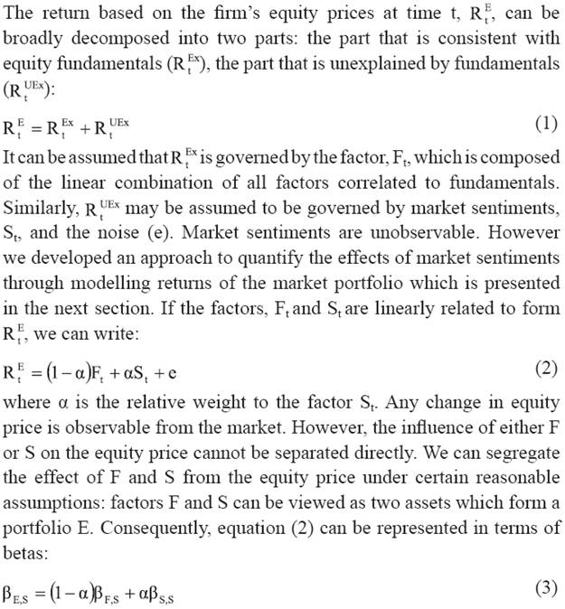
A. The Market Sentiments Our model is based on the basics of isolating effects of non-fundamentals from the equity return. The residual part of which is the component of the equity return governed by the factors which caused a systematic change in it. Therefore, this part can be taken as an input in an asset pricing model. Non-fundamentals would essentially be investors’ sentiments. However, effects of investors’ sentiments are not observable from the market and also never clearly defined in economics literature. According to the theory of capital markets, news/ information released in the market is the driving force behind an investors’ investment decision. However, apart from news/information, an individual investor’s investment decision is also guided by collective beliefs, also termed investors’ sentiments. Investors’ sentiments peak or trough when the market experiences extreme events. We are experienced, in the one extreme, investors’ sentiments render into a panic which may lead a sharp downturn in the market index. In the other extreme, positive sentiments may cause a significant rise in the market index. Therefore, the initial step in modeling market sentiments might be based on the assumption that effects of market sentiment are properly summarised into a diversified market portfolio. However, it is not necessarily implied that sentiments are the only factors behind any ups or downs of market returns. Movements in the market return are essentially due to the combined effects of market fundamentals and collective investors’ sentiments. Consequently, it is not difficult for a researcher to segregate the above two effects by fitting a linear model. We can go back to the basics of asset pricing theory that indicates the market portfolio is a well-diversified portfolio, which is the optimal portfolio for at least one utility-maximising investor. Because of the diversified nature of that portfolio, the nonsystematic risks of each asset sums up net to zero. The only risk that exists in the market portfolio is the systematic risk. Therefore, the return of such a portfolio is regulated by those factors which fuel systematic risk. These factors may be of two types: one linked to fundamentals and others not so linked. Here, unlike the equity of a single firm, fundamentals are more economy-specific than firm-specific. For a given factor structure, we can divide the return of the market portfolio (RtM) into two parts: the part consistent with market fundamentals (RtMx) and the part unexplained by fundamentals (RtUMx):
B. The long run versus short run expectations
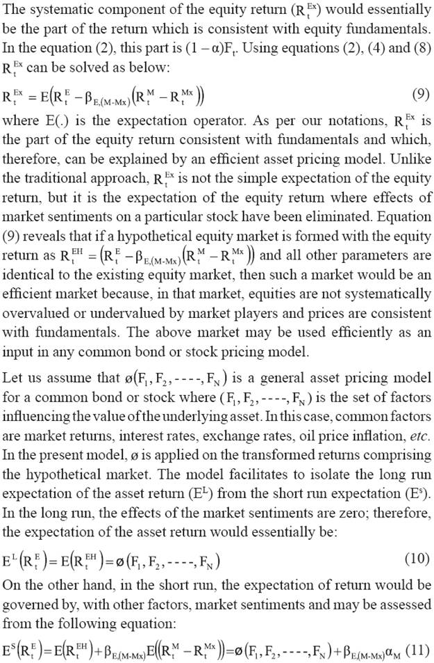
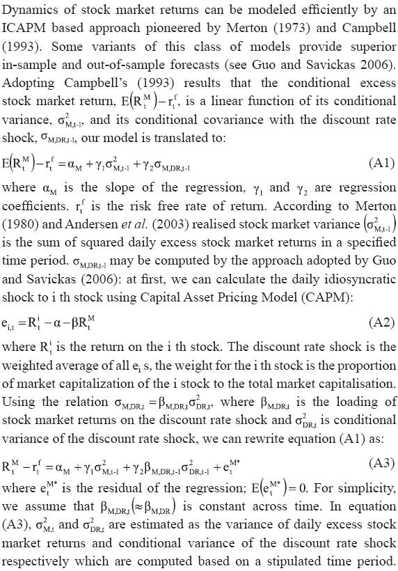
Section IV National Stock Exchange (NSE) in India maintains 11 major indices and 14 sectoral indices, details of which are given in the Annex. These indices are computed on a free float-adjusted market capitalisation weighted methodology which is a popular approach. They are comparable across sectors and, therefore, used extensively in empirical research. Among these major and sectoral indices compiled by the NSE, six indices are selected for our empirical analysis. These indices are: S&P CNX Nifty (P1), CNX Nifty Junior (P2), S&P CNX Defty (P3), Bank Nifty (P4), CNX Midcap (P5) and CNX Infrastructure (P6)2. Based on these indices, applicability of standard asset pricing models is examined by us for Indian markets. These models have been recognised as useful quantitative tools behind an investor’s asset allocation strategies or in monitoring performances of his existing investments. However, these models are useful to the extent they are supported by empirical regularities observed in market returns. Unfortunately, all conventional forms of these models and their empirical validity have been questioned by several scholars over past twenty years (see Bird, Menzies, Dixon, and Rimmer (2010); Majumder (2011)). This tenet of research was the exploration of certain regularities in market returns which were not the fruit of the standard models. Predominant among these observed empirical phenomena would be the predictability of portfolio returns through time. On many occasions, past returns contain additional information about expected asset returns which lead asset returns to be serially correlated. Serial dependence in portfolio returns is evidence in favour of market inefficiency which is examined by us for Indian markets. This test has been performed separately for the original market and the hypothetical market to show that hypothetical market returns are, in general, not auto correlated and so meet the prerequisites of applying an asset-pricing model. Prior to manipulating any asset pricing model for predicting equity returns, it is worthwhile to examine whether the capital market is informationally efficient. One effective way to test this might be through investigating serial correlation properties of equity returns. Such test is also useful to examine existence of investors’ sentiment in the equity market. In the present paper, the test is performed on daily portfolio returns in the similar line of Jegadeesh (1990). The particular cross sectional regression model used in the empirical tests is 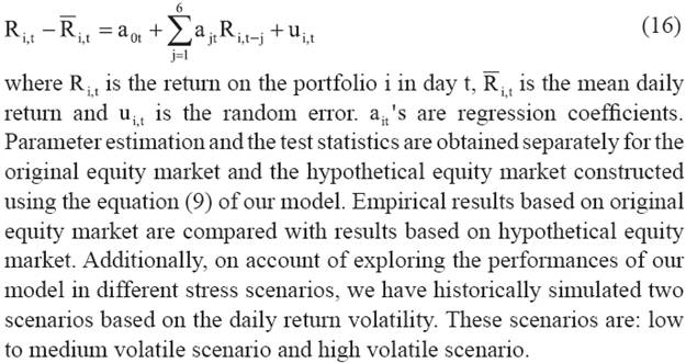 Scenarios can be based on a significant market events in the past (a historical scenario) or on a plausible market event that has yet to happen (a hypothetical scenario). A historical scenario is generated from historical data and is used extensively in financial research (BCBS, 2009). It involves identifying risk factors based on actual historical events. The basic insight of this method is that the events which happened in reality are plausible to reappear. With this method, the range of observed risk factors changes during a historical episode is applied to the portfolio to get an understanding of the portfolio’s risk in case such a situation recurs (Blaschke, et al., 2001, p. 6). We have identified historical events which caused large movements in equity returns in the Indian markets that include equity market crash in May 2004, May 2006, the recent financial crisis that began since July 2007 and many others. Movements in returns as consequences of these events provide the high volatile scenario and if these consequences are separated from the historical dataset, it gives low to medium volatile scenario. The return distribution of a portfolio under a simulated historical scenario is given by the empirical distribution of past returns on this portfolio. Regression model in the equation (16) has been estimated using daily returns over the period January, 2003 to March, 2009 separately for low to medium volatile scenario and high volatile scenario. Results for the original and the hypothetical market are presented in the table 1 and 2 respectively. Table 1 shows that coefficients for one day lagged return are positive and statistically significant for all sampled portfolios in low to medium volatile scenarios and also in high volatile scenario. Moreover, the coefficient, a1, is bigger in absolute magnitude than the rest. The results indicate positive first order auto correlation for returns in the original equity market. In addition to this, table 1 indicates one or more higher order auto correlations are different from zero for almost all portfolios. However, the average R2 of the daily cross-sectional regressions is 0.032; i.e., on average the lagged returns considered here can explain 3.2 percent of the cross-sectional variation in individual security returns. Our results are consistent with the findings of earlier authors (see Kramer, 1998; Blandon, 2007). Narasimhan & Pradhan (2003) tested the validity of CAPM for size based portfolios in Indian markets and they confirmed failure of the model for most of the portfolios. The reason might be over time dependencies of the return series. Contrarily, Table 2 indicates that for almost all occasions, coefficients for lagged returns are not statistically significant for both the scenarios resulting a very low R2 of regression. Therefore, in general, stock returns in the hypothetical market are not auto correlated. The results can be verified further by presenting F-statistics under the hypothesis that all slope coefficients are jointly equal to zero. Table 3 indicates that for the original market almost all F statistics are statistically significant at 5 per cent significant level indicating all slope coefficients are not jointly equal to zero. However, results are opposite for the hypothetical market where most of the F statistics are statistically insignificant. The results indicate that the original equity market returns are auto correlated for at least one lag, however the hypothetical market returns are not so autocorrelated. Over last four decades, empirical research on market efficiency experienced a phenomenal growth covering all sorts of markets ranging from an emerging to a developed one. Paradoxically, findings of many of these studies are contradictory even for the same stock market under study. Indian markets might be prominent examples of this controversy. Conflicting outcomes of econometric tests employed for these emerging markets documented by several authors reveal the fact that market efficiency is often a sample- or situation-dependent phenomenon which makes hard to detect the true nature of these markets. Simultaneously, it becomes difficult to select an asset pricing model which is applicable for these markets. Unfortunately, ‘mispricing’ might be a common outcome of application of any familiar asset pricing model for these markets whose true nature is unknown to the researcher. The foundation for this mispricing is well encapsulated by the words, irrational exuberance/ or pessimism, which reflect a period when emotions take over and valuation plays at best a limited role in determining equity prices. In these circumstances, stock returns become predictable over time. In Indian markets, on many occasions, the daily equity return is significantly predictable by its own past observations. The CAPM, however, cannot explain such predictability. In view of widening the applicability of rational models for asset pricing ranging from an efficient to an inefficient market, we propose a transformation through which the original market would be transformed to a hypothetical market which is relatively efficient. In this framework, we assumed that the equity price today is an outcome of the combined effect of news/information released in the market and subsequent sentiments cultivated by them. The effect of the market sentiment on equity price (or return), however, is unobservable. We developed a model to estimate this component which was subsequently filtered out from original equity returns. The filtered returns were used as inputs in constructing the hypothetical market. In that market, investors’ sentiments cannot induce investors to systematically overvalue/ or undervalue a stock and, therefore, apart from the noise, the equity price (or returns) would be governed only by its fundamental value. In this connection, our empirical study for Indian equity market has established the following: original equity market returns are auto correlated for at least one lag. However the hypothetical market returns are, in general, not so auto correlated. Therefore, transformed returns comprising the hypothetical market meet the prerequisites of applying an asset-pricing model and, therefore, any conventional bond or stock pricing model could be efficiently manipulated for those returns. The approach will widen the scope of asset-pricing models ranging from a strict efficient market to an inefficient market. Appendix: Modeling predictable component of the market return
References Andersen, T., T. Bollerslev, F. Diebold, and P. Labys. (2003), “Modeling and Forecasting Realized Volatility”, Econometrica Vol.71: 579-625. Avramov, D., T. Chordia, and M. Goyal. (2006), Liquidity and Autocorrelations in Individual Stock Returns”, The Journal of Finance Vol. 61: 2365-2394. Barberis, N., A. Shleifer, and R. Vishny. (1998), “A model of investor sentiment, Journal of Financial Economics”, Vol. 49: 307-343. BCBS, Bank for International Settlements (2009). “Principles for sound stress testing practices and supervision”, www.bis.org/publ/bcbs155.pdf. Bird, R., G. Menzies, P. Dixon, and M. Rimmer (2010). “The economic costs of US stock mispricing, Journal of Policy Modeling”, doi:10.1016/j.jpolmod.2010.10.010 Black, F., and M. Scholes (1973). “The pricing of options and corporate liabilities”, Journal of Political Economy, Vol. 81: 637-659. Blandon, J.G. (2007). “Return Auto correlation Anomalies in two European Stock Markets”, Revista de Análisis Económico, Vol. 22: 59-70. Blaschke Winfrid [et al.] Stress Testing of Financial Systems: An Overview of Issues, Methodologies, and FSAP Experiences [Online] // International Monetary Fund. - June 2001. - http://www.imf.org/external/pubs/ft/wp/2001/wp0188.pdf. Cutler, D., J. Poterba, and L. Summers (1989), “What moves stock prices?”, Journal of Portfolio Management Vol. 15: 4–12. Campbell, J. (1993). “Intertemporal Asset Pricing Without Consumption Data”, American Economic Review, Vol. 83: 487-512. Chan, K. (1993). “Imperfect information and cross-autocorrelation among stock prices:, Journal of Finance, Vol. 48: 1211 –1130. Chan, K.C., B.E. Gup, and Ming-Shiun. Pan (1997). “International Stock Market Efficiency and Integration: A Study of Eighteen Nations”, Journal of Business Finance & Accounting, Vol. 24: 803–813. Chang, E.J., E.J.A. Lima, and B.M. Tabak (2004). “Testing for predictability in emerging equity markets”, Emerging Markets Review, Vol. 5: 295-316. Chen, C.R., Y. Su, and Y. Huang (2008). “Hourly index return autocorrelation and conditional volatility in an EAR–GJR-GARCH model with generalized error distribution”, Journal of Empirical Finance, Vol. 15: 789–798. Chopra, N., J. Lakonishok, and J.R. Ritter (1992). “Measuring Abnormal Performance: Do Stocks Overreact?”, Journal of Financial Economics, Vol. 31: 235-268. Conrad, J., and G. Kaul (1988). “Time-Variation in Expected Return”, The Journal of Business, Vol. 61: 409-425. Fama, E.F. (1970). ‘‘Efficient Capital Markets: A Review of Theory and Empirical Work’’, Journal of Finance, Vol. 25: 383-417. Fama, E.F. (1991). “Efficient Capital Markets: II”, Journal of Finance, Vol. 46: 1575-1617. Fama, E.F. (1998). “Market efficiency, long-term returns, and behavioral finance”, Journal of Financial Economics, Vol. 49: 283-306. Fama, E.F., and K.R. French (1988). “Permanent and temporary components of stock market prices”, Journal of Political Economy, Vol. 96: 246-273. Finkelstein, B. (2006). The Politics of Public Fund Investing: How to Modify Wall Street to Fit Main Street. New York: Touchstone Publisher. Gregoriou, A., J. Hunter and F. Wu (2009). “An empirical investigation of the relationship between the real economy and stock returns for the United States”, Journal of Policy Modeling, Vol. 31: 133–143. Guo, H., and R. Savickas (2006). “Understanding Stock Return Predictability”, Working Paper 2006-019B, Federal Reserve Bank of St. Louis. Harvey, C.R. (1995a). “Predictable risk and returns in emerging markets”, The Review of Financial Studies, Vol. 8: 773-816. Harvey, C.R. (1995b). “The Risk Exposure of Emerging Equity Markets”, World Bank Economic Review, Vol. 9: 19-50. Jegadeesh, N. (1990). “Evidence of Predictable Behavior of Security Returns”, The Journal of Finance, Vol. 45: 881-898. Jegadeesh, N., and S. Titman (1993). “Returns to buying winners and selling losers: implications for stock market efficiency”, Journal of Finance 48: 65-91. Knif, J., S. Pynnonen, and M. Luoma (1996), Testing for common autocorrelation features of two Scandinavian stock markets, International Review of Financial Analysis, Vol. 5: 55– 64. Koutmos, G. (1997). “Do emerging and developed stock markets behave alike? Evidence from six Pacific Basin stock markets”, Journal of International Financial Markets, Institutions and Money, Vol. 7: 221–234. Kramer, W. (1998). “Note: Short-term predictability of German stock returns”, Empirical Economics, Vol. 23: 635-639. LeBaron, B. (1992). “Some relations between volatility and serial correlations in stock market returns”, Journal of Business, Vol. 65: 199–219. Leroy, S., and R. Porter (1981). “The Present Value Relation: Test Based on Variance Bounds”, Econometrica, Vol. 49: 555-577. Lintner, J. (1965). “The valuation of risk assets on the selection of risky investments in stock portfolios and capital budgets”, Review of Economics and Statistics, Vol. 47: 13-37. Lo, Andrew.W., and A.C. MacKinlay (1988). “Stock market prices do not follow random walks: Evidence from a simple specification test”, Review of Financial Studies, Vol. 1: 41-66. Majumder, D. (2006). “Inefficient markets and credit risk modeling: Why Merton’s model failed”, Journal of Policy Modeling, Vol. 28: 307- 318. Majumder, D. (2011). “Asset Pricing when market sentiments regulate assets returns: evidence from emerging markets”, Journal of Quantitative Economics, Vol. 9: PP. 89-117. Malkiel, B.G. (2003). “The Efficient Market Hypothesis and Its Critics”, Journal of Economic Perspectives, Vol. 17: 59–82. Malkiel, B.G. (2005). “Reflections on the Efficient Market Hypothesis: 30 Years Later”, The Financial Review, Vol. 40: 1–9. McKenzie, M.D., and R.W. Faff (2005). “Modeling conditional return autocorrelation”, International Review of Financial Analysis, Vol. 14: 23– 42. Merton, R.C. (1973). “An intertemporal capital asset pricing model”, Econometrica, Vol. 41: 867-887. Merton, R. (1980). “On Estimating the Expected Return on the Market: An Exploratory Investigation”, Journal of Financial Economics , Vol. 8: 323-361. Mollah, A.S. (2007). “Testing weak-form market efficiency in emerging market: evidence from Botswana stock exchange”, International Journal of Theoretical and Applied Finance, Vol. 10: 1077-1094. Narasimhan S & Pradhan (2003). “Conditional CAPM and Cross Sectional Returns - A Study of Indian Securities Market” may be downloaded from (http://www.nse-india.com/content/press/jun2003b.pdf). Parametric Portfolio Associates (2008). Emerging Markets: Portfolio structuring to capture long term growth, Emerging Markets Whitepaper, spring, http://www.parametricportfolio.com/. Pesaran, M.H., and A. Timmermann (1995). “Predictability of Stock Returns: Robustness and Economic Significance”, The Journal of Finance, Vol. 50: 1201-1228. Poterba, J., and L. Summers (1988). “Mean Reversion in Stock Prices: Evidence and Implications”, Journal of Financial Economics, Vol. 22: 27-59. Ross, S. (1976). “The arbitrage theory of capital asset pricing”, Journal of Economic Theory, Vol. 13: 341–60. Rubinstein, M. (2001). “Rational markets: Yes or no? The affirmative case”, Financial Analysts Journal, Vol. 57: 15–28. Sharpe, W.F. (1964). “Capital asset prices: A theory of market equilibrium under conditions of risk”, Journal of Finance, Vol. 19: 425-442. Shiller, R.J. (1981). “Do Stock Prices Move Too Much To Be Justified by Subsequent Changes in dividends?”, American Economic Review, Vol. 71: 421-436. Shiller, R.J. (1987). “Fashions, Fads and Bubbles in Financial Markets”, in: Knights, Raiders and Targets, eds., The Impact of the Hostile Takeover, Oxford University Press, UK. On account of monitoring the performance of the overall economy or a sector of the economy National Stock Exchange (NSE), India maintains 11 major indices and 14 sectoral indices:
These indices are computed on a free float-adjusted market capitalisation weighted methodology and are used extensively in empirical research. Historical data for daily closing prices for these indices is available in the NSE-India site. From this list of indices, we have chosen 6 portfolios for our analysis. These portfolios are: S&P CNX Nifty (P1), CNX Nifty Junior (P2), S&P CNX Defty (P3), Bank Nifty (P4), CNX Midcap (P5) and CNX Infrastructure (P6). Data on daily closing prices for these 6 indices for the period January, 2003 to March, 2009 has been downloaded from the above site. * Debasish Majumder is Assistant Adviser (email) in the Department of Statistics and Information Management, Reserve Bank of India. The views expressed in this paper are those of the author alone and not of the institution to which he belongs. 1 Majumder (2006) developed his model for stock pricing in the context of modeling credit risk. 2 Details of these indices are available in the NSE-India site: www.nse-india.com. Daily portfolio price data are obtained from the above site. |


ഈ പേജ് ഷെയർ ചെയ്യുക:


റിസർവ് ബാങ്ക് ഓഫ് ഇന്ത്യ മൊബൈൽ ആപ്ലിക്കേഷൻ ഇൻസ്റ്റാൾ ചെയ്ത് ഏറ്റവും പുതിയ വാർത്തകളിലേക്ക് വേഗത്തിലുള്ള ആക്സസ് നേടുക!
ഞങ്ങളുടെ ആപ്പ് ഇൻസ്റ്റാൾ ചെയ്യാൻ QR കോഡ് സ്കാൻ ചെയ്യുക


പേജ് അവസാനം അപ്ഡേറ്റ് ചെയ്തത്:


