 IST,
IST,


II. Fiscal Position of State Governments
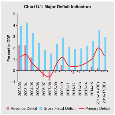
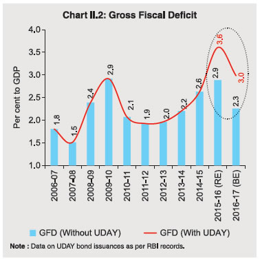
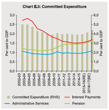
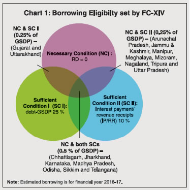
The consolidated fiscal position of states deteriorated sharply during 2014-15 and 2015-16 (RE). Although states budgeted for an improvement in 2016-17 (BE), data for 25 states (RE) show some deterioration in fiscal position. Relaxations in market borrowings provided by the Fourteenth Finance Commission (FC-XIV) have allowed many of the states to mobilise additional resources. Despite the increase in the debt burden of the states in recent years, the overall fiscal position is found to be sustainable in the long run. Based on information pertaining to 25 states, the consolidated gross fiscal deficit to gross state domestic product (GFD-GSDP) ratio is budgeted to moderate to 2.6 per cent in 2017-18. 1. Introduction 2.1 The consolidated finances of states has deteriorated in recent years, with the GFD-GDP ratio averaging around 2.5 per cent in the last five years (2011-12 to 2015- 16) as compared with 2.1 per cent during the previous quinquennium (Table II.1). The GFD-GDP ratio in 2015-16 (RE) breached the 3 per cent2 ceiling of fiscal prudence for the first time since 2004-05. Information on 25 states indicate that the improvement in fiscal metrics budgeted by states for 2016-17 may not materialise. It is expected that states will take necessary steps to consolidate their fiscal position. 2. Accounts: 2014-15 2.2 At the consolidated level, key deficit indicators of states deteriorated in 2014-15 (Chart II.1), with special category (SC) states3 posting the largest erosion (Table II.2). 2.3 On the receipts side, grants from the Centre increased significantly, reflecting changes in the pattern of funding of centrally sponsored schemes (CSS)4. Consequently, enhanced central transfers provided a boost to revenue receipts (Table II.3). On the expenditure side, there was a significant increase in development expenditure (Table II.4). Both revenue and capital expenditure5 increased, the former outpacing the latter. Revenue expenditure rose significantly in respect of items such as education, sports, art and culture, and rural development. Capital expenditure increased on account of growth in capital outlay for items such as housing, dairy development, rural development, and energy. 3. Revised Estimates: 2015-16 2.4 The combined fiscal position of states deteriorated sharply in 2015-16 (RE) from the budgeted estimates for the year. For the first time in more than 10 years, the GFD-GDP ratio at 3.6 per cent crossed the threshold of 3 per cent, but this was mainly due to the significant increase in capital outlay and loans and advances to power projects (Table II.5). The deficit in the revenue account was lower due to revenue receipts in the form of tax collections and states’ own non-tax revenues accelerating over the year and outpacing revenue expenditure. This improvement was also supported by central transfers6; however, the major thrust was through higher devolution of resources from central taxes7. With the steep increase in the GFD, primary deficit (PD) was higher despite a marginal increase in interest payments. While the revenue account deteriorated for 13 states from the previous year; among these, six states continued to maintain surpluses. On the other hand, the GFD worsened for 20 states (Table II.6). 2.5 Capital expenditure expanded by one percentage point of GDP in 2015-16 (RE) with developmental expenditure rising faster than non-developmental spending (Table II.4). Within developmental capital outlay, sectors which saw significant growth were major and medium irrigation and flood control, energy, and roads and bridges, reflecting the intent to create growth-enabling infrastructure. 2.6 Loans and advances for power projects increased significantly as an outcome of the Ujwal Discom Assurance Yojana (UDAY) scheme. Under the scheme, states took over 75 per cent of Discom debt as on September 30, 2015 over two years – 50 per cent in 2015- 16 and 25 per cent in 2016-17. States were allowed to issue non-SLR state development loan (SDL) bonds in the market or directly to banks / FIs holding the Discom debt8. As per the RBI records, 8 states9 borrowed ₹ 989.6 billion under UDAY during 2015-16. Net of these bonds, the consolidated state GFDGDP ratio gets moderated by 0.7 percentage point during 2015-16 to 2.9 per cent from 3.6 per cent in the previous year (Chart II.2)10. 2.7 The growth in revenue expenditure in 2015-16 (RE) drew from higher development revenue expenditure for education, sports, art and culture, social security and welfare, relief on account of natural calamities, rural development and energy. Under non-development expenditure, committed expenditure comprising pensions, interest payments and administrative services rose marginally (Chart II.3). 4. Budget Estimate: 2016-17 2.8 At the aggregate level, the key deficit indicators were budgeted to improve in 2016- 17 (BE) over a year ago. With revenue receipts budgeted higher than revenue expenditure, a small revenue surplus was expected to accrue. Along with a decline in loans and advances, this would have reduced the GFD-GDP ratio in spite of some increase in capital outlay. The consolidated GFD-GDP ratio was budgeted at 3.0 per cent, resulting in a lower budgeted primary deficit than a year ago. 2.9 An analysis of state-wise positions indicates that while 18 out of 29 states budgeted for a revenue surplus, 15 budgeted for an improvement in the revenue account (in terms of GSDP11) from the previous year. Improvement in both the GFD-GSDP and PD-GSDP ratios were budgeted by 16 states (Table II.6). 2.10 Capital outlay was budgeted to account for about 99 per cent of GFD in 2016-17 (BE), reflecting a distinct improvement in the quality of the deficit. Over the years, market borrowings has been a dominant source of financing the GFD. As per RBI records, gross market borrowing of states at ₹ 3,819.8 billion in 2016-17 – comprising around 85 per cent of GFD – increased by 29.7 per cent over the previous year. In contrast, the contributions of National Small Savings Fund (NSSF), reserve funds, deposits and advances have reduced (Table II.7). 2.11 The increasing reliance on market borrowing, along with the enabling conditions for additional borrowing by states as provided by FC-XIV, poses challenges for the sustainability of state finances as higher state borrowings raise yields and the cost of borrowing (Box II.1). The combined gross market borrowings of the Centre and the states increased by 7.1 per cent during 2016-17. Revenue Receipts 2.12 Central transfers as well as states’ own revenue were budgeted to increase in 2016-17. Both components of central transfers, i.e., the share in central taxes as well as grants from the Centre, were budgeted to increase. Some improvement was budgeted in own tax revenue (OTR) and own non-tax revenue (ONTR). The increase in grants in aid was mainly led by the increase in grants for state plan schemes, while own tax revenue was higher on account of higher tax collections through “state sales tax/VAT”. Relaxation of Fiscal Rules for States FC-XIV recommended that the fiscal deficit of all states will be anchored to an annual limit of 3 per cent of GSDP for the award period (2015-16 to 2019-20). Relaxations were, however, given to state governments for additional borrowings provided they met some criteria of fiscal prudence. These criteria can be broadly categorised as a) necessary and b) sufficient conditions12: • Necessary Condition (NC): Availing additional borrowing is contingent upon the state recording a zero revenue deficit in the year for which the borrowing limit has to be fixed and in the immediately preceding year. • Sufficient Conditions (SCs) : An additional borrowing limit of 0.25 per cent each is allowed if: I) SC-I: states’ debt-GSDP ratio is less than or equal to 25 per cent in the preceding year, II) SC-II: interest payment/revenue receipts (IP/RR) is less than or equal to 10 per cent in the preceding year. States meeting one or both of the above criteria are allowed a relaxation in their fiscal deficit targets by 0.25/0.5 per cent of GSDP provided they meet NC. There were seventeen states which satisfied the NC and at least one of the SCs, becoming eligible for additional borrowing in 2016-17. Out of these states, seven satisfied both the SCs and were eligible to have a maximum GFDGSDP ratio of 3.5 per cent in 2016-17. There were ten states which satisfied only one of the SCs, becoming eligible for additional borrowings to the extent of 0.25 per cent of GSDP in 2016-17. Consequently, their GFD-GSDP ratio can increase to a maximum of 3.25 per cent. Information available for 2016-17 suggests that the seven states which actually resorted to additional borrowing can be categorised into three groups: i) states which were eligible for additional borrowing but remained within the prescribed limit; ii) states which were eligible for additional borrowing but crossed the limit; and iii) states which have borrowed without being eligible for additional borrowing as per the above-mentioned criteria. While two states belong to the first category, three states have borrowed more than their respective limits. Finally, two states who were not eligible for additional borrowing also resorted to borrowing during the year.
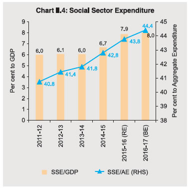
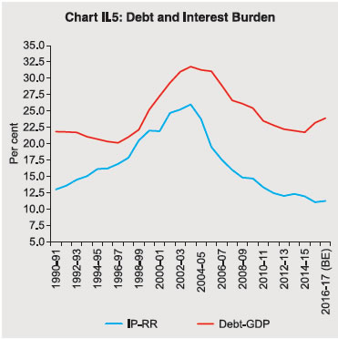
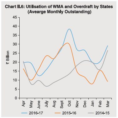
Reference Government of India (2014), “Report of Fourteenth Finance Commission” New Delhi. Expenditure Pattern 2.13 The consolidated revenue expenditure of states was budgeted to increase in 2016-17 (BE) over a year ago. A significant deceleration in development revenue expenditure was budgeted mainly on account of lower growth in expenditure for family welfare, housing, labour and labour welfare, social security and welfare, agriculture and allied activities, and rural development. Furthermore, a decline in revenue expenditure (in absolute terms) was budgeted on items like energy, roads and bridges. In contrast, non-development revenue expenditure was budgeted to increase as committed expenditure continued to remain elevated. 2.14 Capital expenditure was budgeted to be lower in 2016-17 (BE) than in the preceding year mainly due to a decline in loans and advances relating to power projects under the UDAY scheme. Capital outlay was budgeted to increase marginally with some deceleration in the growth in development capital outlay for (i) water supply and sanitation, and (ii) roads and bridges. In contrast, a decline was budgeted in (iii) family welfare, (iv) soil and water conservation, (v) agricultural research and education, and (vi) energy. A lower capital outlay in these critical sectors is a matter of concern. 2.15 Social sector expenditure (SSE) 13was budgeted to increase, as proportions to GDP and aggregate expenditure14 (Chart II.4). Disaggregated data, however, showed that SSE (as proportion to aggregate expenditure) was budgeted to decline in 13 states (Statement 35). The composition of expenditure on social services showed that more than 60 per cent was allocated for spending on education, sports, art and culture, and medical and public health, which will have a positive bearing on social infrastructure (Table II.8). 5. Budget Estimates: 2017-18 2.16 As per the information available for 25 states, the GFD-GSDP ratio is budgeted at 2.6 per cent during 2017-18 as compared with 3.4 per cent during 2016-17 (RE). There are, however, several downside risks like implementation of recommendations of states’ own pay commissions, farm loan waiver in some states, and revenue uncertainty on account of the implementation of GST. On a comparable basis, the revised estimates of the GFD for 2016-17 were higher by 0.4 percentage point over the budgeted ratio – raising concerns about potential fiscal slippage (Table II.9). 6. Outstanding Liabilities of State Governments 2.17 Outstanding liabilities of state governments have been registering double digit growth since 2012-13, except in 2014-15. UDAY inter alia caused outstanding liabilities to increase by 1.5 percentage points of GDP in 2016 over 2015 and by 0.7 percentage point in 2017 over 2016 (Table II.10). State-wise data reveal that the debt-GSDP ratio increased for 17 states (Statement 20). 2.18 The interest payments-revenue receipts (IP-RR) was budgeted to rise marginally in 2016-17 (BE), reflecting higher interest burden on account of UDAY bonds (Chart II.5). Composition of Debt 2.19 The composition of states’ outstanding liabilities indicates greater reliance on market borrowings over the years – they constituted 69.7 per cent of outstanding liabilities of states at end-March 2015 and was budgeted to reach 74.7 per cent by end-March 2017. The share of NSSF in outstanding liabilities and states’ dependence on loans from the Centre, however, continued to decline (Table II.11). 2.20 The weighted average yield on state government securities moderated to 7.48 per cent in 2016-17 from 8.28 per cent in 2015-16. The spread of yields on State Development Loans (SDLs) over the benchmark 10-year Central Government security yield remained broadly stable in the range of 24-114 basis points in 2016-17 as against 21-109 basis points in 2015-16. The weighted average spread of SDLs firmed up by 59 basis points in 2016-17 as compared with 50 basis points in 2015-16. Among the states, Punjab consistently issued securities of 4 and 5 years tenor, utilising borrowing space in the medium-term maturity bucket. Other states such as Andhra Pradesh, Gujarat, Maharashtra and Odisha also issued securities of less than 10 year maturity. States issuing securities of more than 10 year maturity during 2016-17 included Andhra Pradesh, Maharashtra, Telangana, Odisha and Union Territory of Puducherry. Maturity Profile of State Government Securities 2.21 As at end-March 2017, 68.0 per cent of the outstanding SDLs were in the residual maturity bucket of five years and above (Table II.12). The redemption of special securities issued under financial restructuring plans (FRPs) for state-owned Discoms entails large repayment obligations from 2018-19. Special securities issued under FRPs are significantly larger in size; consequently, repayment pressure will be aggravated from 2018-19. Power bonds, which were issued to clear outstanding overdues of state electricity boards to the central public sector undertakings (CPSUs), have, however, been extinguished by 2015-1615. Liquidity Position and Cash Management 2.22 Several states have been accumulating sizeable cash surpluses in recent years. As a result, liquidity pressures were confined to few states during 2016-17. States’ intermediate treasury bills (ITB) balance was ₹ 1560.59 billion during 2016-17 as against ₹ 1205.82 billion during 2015-16 while balances on auction treasury bills (ATB) were placed at ₹ 366.02 billion. States availed higher ways and means advances (WMA) and overdrafts (ODs) more sizably in 2016-17 than in the previous year (Chart II.6). 2.23 The rise in debt burden of the states in the last couple of years has drawn attention to the sustainability of public debt at the subnational level. In view of this, the following section provides an assessment of the debt sustainability of state governments over the medium to long run. 7. Debt Sustainability of Indian States 2.24 State governments face severe resource constraints as their non-debt receipts are often insufficient for fulfilling their developmental obligations. As a result, they resort to market borrowings to bridge the resource gap. Over a period of time, such borrowings may result in the accumulation of debt liabilities which, if unchecked, could pose major challenges for macroeconomic and financial stability. State Government Debt 2.25 The evolving debt position of states has seen several phases: a comfortable position prior to 1997-98, followed by sharp deterioration and fiscal stress till 2003-04, then significant improvement since 2004-05 albeit with marginal deterioration in the last two years. While the debt liabilities of states increased sharply during 1997-98 to 2003- 04, the subsequent consolidation is attributed inter alia to the implementation of Fiscal Responsibility and Budget Management (FRBM) Acts at the state level during the last decade. These initiatives were complemented by debt and interest relief measures by the Central Government and supported by a favourable macroeconomic environment. Majority of the states adhered to the debt targets set by the FC-XIII for the period 2010- 2014; however, some breached their targets and were saddled with unsustainable debt positions. Assessment of Debt Sustainability 2.26 The path of the primary deficit can be sustainable if the real growth of the economy is higher than the real interest rate (Domar, 1944). The level of debt is considered to be sustainable if a country’s debt-GDP ratio remains stable; and if the economy generates adequate debt-stabilising primary balance to service the future debt (Buiter, 1985; Blanchard, 1990). 2.27 In the empirical literature, there are primarily two approaches to fiscal/debt sustainability. The first evaluates various indicators of the sustainability of fiscal policy (Miller 1983; Buiter 1985, 1987; Blanchard 1990; Buiter et al. 1993), while the second involves empirical validation or tests of government solvency (Hamilton and Flavin 1986; Trehan and Walsh 1988; Bohn 1998). Empirical testing inter alia include determination of the sustainable (long-run and maximum) level of public debt based on a partial equilibrium framework, a model-based approach and the signals’ approach to fiscal sustainability. While indicators are forward-looking, empirical validation through econometric tests based on historical data are considered backward looking. As a result, a combination of both these approaches has been suggested for drawing additional insights on government solvency (Marini and Piergallini, 2007). 2.28 In the Indian context, empirical studies on debt sustainability of states indicate a mixed picture. While some of the earlier studies point out that the debt position of states are unsustainable (Buiter and Patel 1992; Goyal et al. 2004; Misra and Khundrakpam 2009), the more recent ones have drawn attention to the declining debt-GSDP ratios and attributed this improvement to the strong growth performance and the implementation of fiscal rules during 2003-2012 (Dasgupta et al. 2012; Makin and Arora 2012; Kaur et al. 2014). Consequently, any slowdown in growth over the medium-term could pose risk to the achievement of the GFD-GDP and debt-GDP targets. 2.29 Traditionally, debt sustainability analysis takes into account credit-worthiness (nominal debt stock/own current revenue ratio; present value of debt service/own current revenue ratio) and liquidity indicators (debt service/ current revenue ratio and interest payments/ current revenue ratio). These indicators broadly provide an assessment of the ability of state governments to service their debt (interest obligations and repayment) through current and regular sources of revenue. 2.30 An analysis based on various indicators of debt sustainability in different phases during the period 1981-82 to 2015-16 reveals that the rate of growth of debt of states at the aggregate level exceeded nominal GDP growth rate during Phase I, Phase III and Phase V (Table II.13). The Domar stability condition was satisfied in all phases, except Phase III. Both primary balance and primary revenue balance remained negative in all the phases, even as there was some improvement in primary revenue balance-GDP ratio in the last two phases. The tolerable limit of average interest payments to revenue receipts ratio of 20 per cent (Dholakia et al. 2004) was breached in Phase III but subsequently came down in Phase IV and further in Phase V. 2.31 The fiscal/debt sustainability exercise is extended beyond the simple indicator-based assessment to empirically validate whether the state governments would remain solvent.This entails test of stationarity properties of the government debt stock, examination of the long-term relationship between government revenues and expenditures, between primary balances and debt, and between capital expenditure and public debt (Bhatt, 2011). While confirmation of stationarity of debt stock (in level and first difference) indicates mean reversion after temporary disturbances, cointegration between government revenues and expenditures is reflective of co-movement, which is essential for satisfying the inter-temporal budget constraint. Empirical assessment of the inter-temporal budget constraint in a panel data framework covering 20 Indian states for the period 1980-81 to 2015-16 indicates sustainable debt position of states in the long run (Box II.2). Debt Sustainability of Indian States – Inter-Temporal Budget Constraint Approach Drawing from the empirical literature, fiscal sustainability is analysed from the perspective of satisfying the intertemporal budget constraint. This requires that government expenditure, revenues and debt stock are all stationary in their first differences [I(1)]. The stationarity property also restricts the extent of deviation of government expenditure from revenues over time. In case government expenditure and revenues are I(1) and cointegrated, then the error correction mechanism would push government finances towards the levels required by the inter-temporal budget constraint and ensure fiscal and debt sustainability in the long term (Cashin and Olekalns, 2000). First, the stationarity properties of state government debt, revenues and expenditure (logarithmic transformation and in real terms) are tested through panel unit root tests for the period 1980-81 to 2015-16 covering 20 Indian states16. The results of panel unit root tests (Levin, Lin and Chu; Im, Pesaran and Shin; and Maddala and Wu test statistics) reveal that the three variables viz., debt, total revenues and total expenditure are I(1). Second, since both revenue and expenditure were found to be I(1), an attempt is made to test whether there exists a long-run equilibrium (steady state) relationship between government expenditure and revenues through panel cointegration tests. Using the extant methodology (Pedroni,1999), the test results for both the panel and group statistics reveal strong evidence of panel cointegration (Table 1). The estimated ‘Rho’ statistics, variance ratio ‘V’ statistics, Augmented Dickey Fuller ‘t’ statistics and the Phillips and Perron (non-parametric) ‘t’ statistics reject the null hypothesis of no cointegration at 1 per cent level for all the three models. Thus, the overall findings of the panel cointegration tests reveal that government revenues and expenditure are cointegrated, indicating long-term co-movement. Along with the stationary property, these results suggest that the current fiscal policies pursued by states are sustainable in the long run, which is in line with recent findings (Kaur et al., 2014). Reference (i) Cashin, Paul and Nilss Olekalns (2000): “An Examination of the Sustainability of Indian Fiscal Policy”, University of Melbourne Department of Economics Working Papers No. 748. (ii) Kaur, B., Mukherjee, A., Kumar, N. and A.P. Ekka (2014): “Debt Sustainability at the State Level in India”, RBI Working Paper Series No. 07. (iii) Pedroni, P. (1999): “Critical Values for Cointegrating Tests in Heterogeneous Panels with Multiple Regressors”, Oxford Bulletin of Economics and Statistics, 61 (1). 8. Concluding Observations 2.32 After a gap of more than 10 years, the GFD-GDP ratio crossed 3 per cent in 2015-16 (RE) despite some moderation in the revenue deficit. Mitigating factors were reflected in higher provisioning for capital outlay and loans and advances. A budgeted surplus in the revenue account and a decline in loans and advances were expected to help reduce the GFD-GDP gap in the budget estimates of 2016-17. 2.33 Information pertaining to 25 major states indicates slippage in the deficit indicators in 2016-17 (RE) from the budget estimates. These states, however, have projected an improvement in their fiscal position in 2017-18 (BE). It is pertinent to note that many state governments are in the process of setting up their pay commissions which may impact projected deficit indicators. 2.34 Notwithstanding the deterioration of the debt position of state governments in the preceding two years due to their participation in the financial and operational restructuring of state power distribution companies through UDAY, empirical evaluation reveals that the current fiscal policies of states are sustainable in the long run. 2.35 Due to prevailing uncertainty about the revenue outcome from the GST implementation, the outlook for revenue receipts of states could turn uncertain. There is, however, the cushion of compensation by the Centre for any loss of revenue for the initial five years. In this context, GST remains the best bet for states in clawing back to the path of fiscal consolidation over the medium term. From this perspective, the current report focusses on the GST as its theme which is discussed in the following chapter. 1 The analysis of various fiscal indicators is in proportion to GDP, unless stated otherwise. Moreover, the analysis pertains to Final Accounts for 2014-15, Revised Estimates (RE) for 2015-16 and Budget Estimates (BE) for 2016-17. 2 The threshold of 3 per cent GFD-GSDP ratio was first recommended by the Twelfth Finance Commission (FC-XII) and later endorsed by both the Thirteenth Finance Commission (FC-XIII) as well as the Fourteenth Finance Commission (FC-XIV). It has also been acknowledged by state governments in their respective Fiscal Responsibility and Budget Management (FRBM) Acts. At the consolidated state level, 3 per cent of GFD-GDP ratio was previously breached in 2004-05. 3 Of the twenty nine states, there are eleven special category (SC) states and eighteen non-special category (NSC) states. The SC states include Arunachal Pradesh, Assam, Himachal Pradesh, Jammu and Kashmir, Manipur, Meghalaya, Mizoram, Nagaland, Sikkim, Tripura and Uttarakhand while NSC states are Andhra Pradesh, Bihar, Chhattisgarh, Goa, Gujarat, Haryana, Jharkhand, Karnataka, Kerala, Madhya Pradesh, Maharashtra, Odisha, Punjab, Rajasthan, Tamil Nadu, Telangana, Uttar Pradesh and West Bengal. 4 Prior to 2014-15, funds under CSS were transferred through the dual mode of i) state budgets; and ii) direct transfer to district rural development agencies and independent societies. In this regard, state governments had expressed their concern as direct transfers to the implementing agencies circumvented the state budgets. To address this issue, the entire financial assistance to the states for CSS is being routed from 2014-15 through the consolidated funds of the states. 5 Capital expenditure includes both capital outlay and loans and advances. 6 Central transfers include share in central taxes and grants. 7 The Union Government accepted the recommendations of FC-XIV to increase the states’ share in the divisible pool of taxes to 42 per cent (earlier 32 per cent) from 2015-16 onwards. It altered the composition of central transfers in favour of statutory transfers from discretionary transfers made earlier. It also led to greater predictability and certainty in the quantum of funds being transferred to the states; additionally, there would be an overall increase in untied funds. 8 See ‘Box IV.1: UDAY Scheme – Salient Features’ published in State Finances : A Study of Budgets 2015-16, Reserve Bank of India. 9 The 8 states are Bihar, Chhattisgarh, Haryana, Jammu & Kashmir, Jharkhand, Punjab, Rajasthan and Uttar Pradesh. 10 As per the UDAY scheme, the debt taken over by the states will not be included in the calculation of their respective fiscal deficit for the financial years 2015-16 and 2016-17. (Government of India, November 5, 2015). 11 While the consolidated fiscal position of all states are analysed in terms of GDP, state-wise analysis is based on the respective gross state domestic product (GSDP) of states. 12 While FC-XIV has not used the terms “necessary” and “sufficient”, these have been used here to simplify the explanation of the condition while retaining its essence. 13 Includes expenditure on social services, rural development, food storage, and warehousing. 14 Includes revenue expenditure, capital outlay, and loans and advances. 15 In order to clear outstanding overdues of state electricity boards to the central public sector undertakings (CPSUs), power bonds aggregating ₹336 billion were issued by state governments with retrospective effect from October 1, 2001 in 20 equal tranches to facilitate trading and redemption of the bonds. Each part carried a fixed tenor with bullet redemption, the last being on April 1, 2016. 16 The states covered are Andhra Pradesh, Assam, Bihar, Gujarat, Haryana, Himachal Pradesh, Jammu & Kashmir, Karnataka, Kerala, Maharashtra, Manipur, Meghalaya, Madhya Pradesh, Odisha, Punjab, Rajasthan, Tamil Nadu, Tripura, Uttar Pradesh and West Bengal, for which data on all the relevant variables are available for the entire time period. In the case of Bihar, Uttar Pradesh and Madhya Pradesh, the data on respective fiscal variables from 2000-01 also include data relating to Jharkhand, Uttarakhand and Chhattisgarh, respectively. This has been done to ensure comparability of data for the entire period covered in the econometric exercise. |

ഈ പേജ് ഷെയർ ചെയ്യുക:


റിസർവ് ബാങ്ക് ഓഫ് ഇന്ത്യ മൊബൈൽ ആപ്ലിക്കേഷൻ ഇൻസ്റ്റാൾ ചെയ്ത് ഏറ്റവും പുതിയ വാർത്തകളിലേക്ക് വേഗത്തിലുള്ള ആക്സസ് നേടുക!
ഞങ്ങളുടെ ആപ്പ് ഇൻസ്റ്റാൾ ചെയ്യാൻ QR കോഡ് സ്കാൻ ചെയ്യുക


പേജ് അവസാനം അപ്ഡേറ്റ് ചെയ്തത്:


