Press Release

Pulses Inflation in India: A Study of Gram, Tur and Moong

Shyma Jose, Sanchit Gupta, Manish Kumar Prasad, Sandip Das, Asish Thomas George, Thangzason Sonna, D. Suganthi and Ashok Gulati¹

Abstract

Utilising primary survey-based information and secondary data, this study employs a monthly balance sheet approach to comprehend the value chain of major pulses - gram, tur, and moong - alongside their price dynamics. In assessing the value chains, the study estimates that approximately 75 per cent of the consumer rupee spent on gram (chana) circulates back to farmers, while the share is around 70 per cent for moong and 65 per cent for tur. The study evaluates supply and demand dynamics through the monthly stock derived from inventory levels, production, consumption and trade. The study assesses relationship between stock-to-use (STU) ratio and consumer price index (CPI) of the three pulses using Autoregressive Distributed Lag (ARDL) models. The empirical analysis shows an inverse relationship between the STU ratio and CPI of gram. The study also forecasts inflation in these pulses over 12-month horizon using both univariate and multivariate time-series models, integrating the STU variable. Empirical evaluations indicate a generally superior performance of the Seasonal Autoregressive Integrated Moving Average with Exogenous Factors (SARIMAX) model incorporating the balance sheet variable across the forecast horizons for the three pulses.

JEL Classification: E31, E37, E52, Q11, Q17, C3

Keywords: Balance sheet, Pulses, SARIMAX, Stock-to-use, Value Chain

Introduction

Food and beverages group constitutes about 46 per cent of the CPI basket in India.²The high share of food in CPI, and the greater susceptibility of food to supply shocks, poses a major challenge for robust inflation projections, which serve as the nominal anchor for monetary policy in a flexible inflation targeting (FIT) regime³(Raj et al., 2019 and Benes et al., 2016). This makes it essential to have an improved understanding of food inflation and its key sources and drivers.

During 2002-03 to 2022-23, there were four major episodes of high and volatile retail food price inflation in double digits (more than 10 per cent) in India. These four phases span over the period 2008-09, 2009-10, 2012-13 and 2013-14. The pre- COVID FIT period witnessed relatively moderate food inflation, barring occasional spikes on account of volatile vegetables prices. The post-2020 period witnessed periods of high food inflation - averaging 7.6 per cent between March-October 2022 and 8.2 per cent during July-December 2023 - on account of supply disruptions caused by geopolitical tensions and adverse climate events.

Elevated inflationary pressure attracts urgent policy attention as it affects household purchasing power and inflation expectations, especially among poor consumers who spend a major portion of their income on food4(Bhattacharya and Sengupta, 2015). Bhattacharya and Jain (2020), while citing the theoretical literature, suggested that stabilising consumption by targeting relative prices of food to non-food (Aoki, 2001), the real income of the farmers (Anand et al., 2015) and the real exchange rate (Catao and Chang, 2015) allows the economy to reach the optimal level of welfare. Anand et al. (2015) illustrates that targeting core inflation (excluding food and fuel) for a developing economy could not result in welfare improvement, especially when the share of food expenditure is high. In addition, food price volatility could lead to second-round effects (Anand et al., 2014; Benes et al., 2016 and Walsh, 2011).

There are many empirical studies that have tried to identify the main drivers of food inflation. Gulati et al. (2013) and Gulati and Saini (2013) have examined the impact of rural wages, fiscal deficit, international food prices and various government policies on food inflation in India. The authors have emphasised the need to boost the supply response in agricultural markets and reduce wastage in supply chains through structural and institutional reforms. Studies such as Bhalla et al. (2011), Kapur and Behera (2012) and RBI (2018) estimated a strong and positive relationship between Minimum Support Price (MSP) and food inflation in India. According to Sonna et al. (2014), real wage, demand for protein-rich items, MSP and input costs were instrumental in driving food inflation during the 1990s and 2000s.

In India, food inflation is also driven by structural factors such as bottlenecks in the food supply chain. Ganguly and Gulati (2013) analysed a mix of demand-side factors, including rising rural wages with the expansion of Mahatma Gandhi National Rural Employment Guarantee Act 2005 (MGNREGA) wages and farm loan waiver, along with supply-side factors such as adverse weather conditions and climate change for understanding food price fluctuations. According to them, subsidy bills and farm loan waivers that increased fiscal deficit contributed to rising food inflation during the 2008-09 crisis, while restrictive trade policies in major exporting economies with the aim of increasing their food security also played a role. The geopolitical tensions due to the war in Ukraine and subsequent export restrictions imposed by a number of countries on food commodities and major agricultural inputs⁵increased food inflation (measured by y-o-y changes in FAO Food Price Index) from 19.7 per cent to 30.3 per cent, and cereals inflation from 12.5 per cent to 34.4 per cent, between January to April 2022 (FAOSTAT).

Being one of the most volatile and price sensitive items within food, understanding pulses price inflation is critical. This study is expected not only to contribute to the literature on food inflation but also to help deepen the understanding of pulses price dynamics with a view to strengthening short-term inflation forecasts of three major pulses (tur, gram and moong). This requires a comprehensive approach taking into account factors that affect the demand for and supply of pulses. Therefore, the study aims to build monthly balance sheets for each of the three pulses to capture the whole gamut of factors – supply and availability with all the processes involved like area sown, production, harvests and arrivals, climatic conditions, wastages and losses, imports, and seasonality on one hand, and consumption requirement of households, income, market dynamics, value chain and role of intermediaries and their behaviour on the other.

Pulses are an affordable dietary protein source in the country. Recent years, however, have witnessed spikes in their prices as a result of demand-supply gap, resulting in large imports. India is the largest producer of pulses, accounting for a quarter of the global pulses production (FAOSTAT) (Chart 1 )⁶and the largest consumer of pulses (with a share of 27 per cent of world consumption) (Mohanty and Satyasai, 2015). Importantly, the demand for pulses has risen considerably in recent years (Abraham and Pingali, 2021; Rampal, 2017 and John et al., 2021). The total pulses consumption increased from 705 grams per capita per month to 783 grams per capita per month in the rural areas and from 824 grams to 901 grams per capita per month in the urban areas between 2004-05 and 2011-12 as per the National Sample Survey Office (NSSO) (GoI, 2012).⁷The estimated price elasticity of pulses varies from (-) 0.70 for poor households to (-) 0.35 for high income households, with an average value of (-)0.46, which implies that in the case of a rise in prices, pulses consumption would decline, and poorer households could be adversely affected (Kumar, 2017).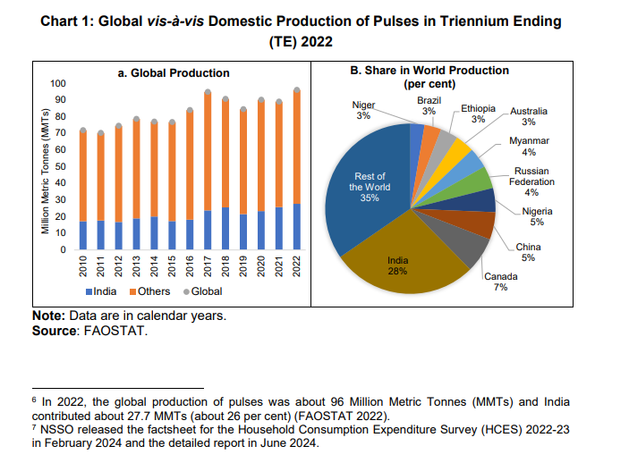

However, for many years, domestic pulses production remained inadequate compared to annual consumption, leading to recurring shortages that were met by imports. India was the largest importer of pulses, accounting for 13 per cent of the total global imports in TE 2022 (2.5 Million Metric Tonnes (MMT)) as per the latest data from FAOSTAT. Canada, Myanmar, USA, Russia and Australia are the major pulses exporters to India. In TE 2022-23, pulses imports were more than 9 per cent of domestic production; the share had touched more than 35 per cent of the production during 2015-16 when domestic pulses production had declined to 16.3 MMT (See Annexure A1).

Pulses are grown in both rabi and kharif seasons. During TE 2023-24, rabi pulses contributed around 67 per cent of total pulses production (as per the second advance estimates (SAE) of 2023-24). Among the major varieties, gram and lentil (masur) are exclusively rabi varieties, and tur is an exclusive kharif variety. Besides, pulses require limited water and most of the area under pulses is rainfed⁸and contributes to improved soil quality through nitrogen fixing.

In the TE 2023-24, eight states – Madhya Pradesh, Rajasthan, Maharashtra, Uttar Pradesh, Karnataka, Andhra Pradesh, Gujarat and Jharkhand - contributed close to 90 per cent of the total pulses production in the country. In terms of yield, there has been progress between TE 2000-01 and TE 2023-24 from 0.56 to 0.90 tonnes per hectare (tonnes per ha). There are, however, wide variations in yield across states. Against the country’s average yield of 0.90 tonnes per ha in TE 2023-24, the top three states in terms of output – Madhya Pradesh, Rajasthan and Maharashtra (which contributed more than 55 per cent of the total production of pulses) have a yield of

1.12 tonnes per ha, 0.66 tonnes per ha and 0.93 tonnes per ha, respectively.

Of all the pulses grown in India, gram (chana/chickpea), a rabi crop, has the largest share in total production (49.5 per cent in TE 2023-24), followed by tur (14.1 per cent). Gram comes in several varieties, with the garbanzo bean (referred to as kabuli chana in India) being commonly found worldwide. Another type of gram produced in India, referred to as Bengal gram or desi chana, accounts for about 80 per cent of Indian gram production.⁹Madhya Pradesh, Maharashtra and Rajasthan contributed more than 65 per cent of the total gram production in TE 2023-24. Gram is mostly inter-cropped with mustard, sunflower, wheat, linseed and coriander.

The second important pulse, tur (arhar), also referred to as pigeon pea, is a kharif crop with a crop cycle of 160 to 180 days. Tur is grown under rainfed conditions in Maharashtra, Karnataka, Uttar Pradesh, Gujarat, Madhya Pradesh, Jharkhand and Telangana. Tur is mostly intercropped with cereals (sorghum, millets and maize), oilseeds, short-duration grain legumes (pulses), or cotton. Although India produced

3.6 million tonnes of tur annually in TE 2023-24, around 20 per cent of the domestic demand for tur was met through imports, mostly from Mozambique, Malawi and Myanmar.

Moong is the third important variety of pulses (after gram and pigeon pea) grown, accounting for 10.7 per cent of total production in TE 2023-24 as per the SAE for 2023-24.¹⁰The crop is grown along with maize, pearl millet, pigeon pea and cotton. Moong varieties are grown in three seasons – kharif, rabi and summer. Furthermore, being a short duration crop, moong is suitable for crop rotations and is mostly produced in Rajasthan, Madhya Pradesh, Maharashtra and Karnataka. Moreover, being a rainfed crop, moong and gram induce a degree of variance in its production in each state.

The distribution channels for raw pulses encompass both institutional and non- institutional avenues. These avenues encompass direct transactions between farmers and traders/processors, farmers selling their produce to traders/processors at mandis (local markets), and procurement activities executed by the farmers' cooperatives as well as National Agricultural Cooperative Marketing Federation of India Limited (NAFED). Non-institutional channels involve numerous intermediaries, such as traders, wholesalers, commission agents, millers, and retailers. Over the years, the government has undertaken different strategies to manage domestic supplies of pulses as well as contain pulses inflation, which includes augmenting supply by raising production incentives under programmes like the National Food Security Mission (NFSM), incentivising domestic production by raising minimum support prices (MSPs), creating a buffer stock of pulses by undertaking procurement of different pulses, which is later on offloaded in the markets to contain price pressures; invoking the Essential Commodities Act (ECA) and imposing stocking limits on pulses, and manoeuvring the trade policy while ensuring continued remunerative prices for farmers.

Against this backdrop, the present paper tries to identify key factors determining pulses prices, particularly for the three main varieties of pulses grown in India – gram (chana), pigeon pea (tur/arhar), green gram (moong). It provides insights into the changing market dynamics and the role of supply management measures in containing price pressures on pulses. Specifically, the main objectives of the study are:

1. To create a dynamic balance sheet that explains the monthly supply and demand situation of the commodities, which can be used for empirical analysis. For this purpose, stock-to-use (STU) ratio has been constructed from the balance sheet;
2. To empirically estimate the determinants of gram, tur and moong prices using macro and commodity specific variables derived from the balance sheet;
3. To forecast inflation of gram, tur and moong for up to 12 months ahead and evaluate the performance of the different forecasting models; and
4. To understand the complex value chains of the three pulses to provide policy suggestions for stabilising prices as well as raising farmers’ share in the consumer rupee.¹¹

The estimation of price mark-ups and share of farmers in the consumer rupee shows that for gram, approximately 75 per cent of the consumer rupee spent on chana is received by the farmers. This percentage is around 70 per cent for moong and 65 per cent for tur. Farmers get a larger share of the consumer rupee for pulses as compared to other commodities like vegetables and fruits as they are non-perishable with relatively longer shelf life (Bhoi et al., 2019 and Suganthi et al., 2024). Pulses can be stocked for more than a year, which in turn, renders pulses stock as an important determinant of price.

The study assesses relationship between STU derived from the balance sheet and CPI of gram, tur and moong using autoregressive distributed lag (ARDL) models. The empirical analysis shows an inverse relationship between STU ratio and CPI of gram. Similarly, the market dynamics variable (Mark), which is deviations of the respective margins between retail and wholesale prices from the respective pulses price momentum, were found to be contributing positively to prices of tur and moong.

The rest of the paper is organised into six sections. Section II discusses in detail the broad literature that becomes the base for our analytical framework to understand pulses inflation. Section III discusses the data sources. Section IV provides an overview of, inter alia, supply management measures taken over the last decade, trends in pulses inflation and seasonality in prices of gram whole, tur and moong. Section V deals with the identification of the stakeholders in gram, tur and moong value-chain, maps their activities and estimates price mark-ups in the pulses value chain. Section VI presents the methodological framework used in constructing the monthly balance sheets and the structural estimation of the respective commodity’s price dynamics. Section VII concludes and provides policy suggestions to contain pulses price volatility.

II. Review of Literature and Analytical Framework to Understand Pulses Inflation

Several studies have empirically identified the factors driving food inflation in India, which can be broadly categorised into demand and supply-side factors. Largely, the demand side factors for food inflation include rising per-capita income due to a sharp increase in rural wages with indexation of MGNREGA wages coupled with pay commissions awards to workers (Sekhar et al., 2018 and Gulati and Saini, 2013), increase in monthly per capita expenditure (Bhattacharya and Sengupta, 2018 and Nair and Eapen, 2012), level of MSP (Sonna et al., 2014 and Nair and Eapen, 2015), lagged impact of expansionary monetary and fiscal policy (Rangarajan and Sheel, 2013; Ganguly and Gulati, 2013 and Gopakumar and Pandit, 2017) and diversification of Indian diet towards high-valued agricultural products (RBI, 2011; Nair and Eapen, 2012 and Gokarn, 2011).

Several factors affect supply-side conditions. These include production fluctuations due to agro-climatic risk, drought or flood (Mohanty, 2014); increasing cost of production (Sonna et al., 2014) due to increase in domestic oil prices and fertiliser cost (Bhattacharya and Gupta, 2018 and Nair and Eapen, 2012); disruption in agri- food supply chain due to pandemic (Narayanan, 2022); and international prices and restrictive trade policies by major exporting countries (Bhattacharya and Sengupta, 2018). Abraham and Pingali (2021) found that non-price factors, including adverse weather vagaries and institutional issues related to market access along with technological change, have a relatively higher impact on supply than price factors in India.

While studying high-value commodities such as pulses, milk, meat, fruits and vegetables with an income elastic demand, Nair and Eapen (2012) emphasise that the persistent price pressure is due to structural factors i.e., poor supply response to rapidly increasing demand. The literature emphasises that price stability in food necessitates the demand or supply function to be elastic. Sekhar et al. (2018) highlighted two short-run supply relations that are important to understand the production responsiveness of farmers to changing demand. The first supply function is where there is a time lag between the farmer’s production decision and actual production. The second supply function is when supply is completely inelastic for a shorter time period and production cannot be changed particularly in the case of perishable commodities. A study by Nerlove (1958) highlighted that actual production is a function of past production, expected prices and other supply factors, which can be captured through a partial adjustment model.

Studies such as Abraham and Pingali (2021) found that the response of sown area response to prices is inelastic in India, however productivity and prices of competing crops, access to irrigation and rainfall impacts pulses prices. The paper further reiterates that volatility in pulses availability and prices will persist in the country if pulses production remains semi-commercial with lower market access to farmers, and supply remaining responsive to exceptionally high prices. Joshi et al. (2017) found that pulse farmers make their sowing choices based on the prices they have seen in the preceding period. Consequently, they may overproduce or underproduce crops, leading to cyclical fluctuations in prices.

Sekhar et al. (2018) found that supply and demand-side factors were equally important in explaining inflationary pressures in pulses. Specifically, production, wage rate and monthly per capita expenditure had a significant impact. In a similar vein, Gopakumar and Pandit (2017), while studying factors impacting high inflation in protein products using a structural simultaneous equation model for the period from 1980-81 to 2013-14, estimated that the lag of increased supply, growth of income and increased money supply, capital formation in the agricultural sector and relative prices of a substitute commodity have a significant impact on pulses inflation. Furthermore, the study highlighted that domestic demand for pulses is met through imports and therefore, with no trade restrictions, international price movement can significantly impact domestic availability and price stability of pulses. Notably, the study recommended that inflation targeting policies for pulses should focus on supply-side management by increasing their availability.

Studies have also incorporated supply chain issues and mark-up charged at different levels of the value chain from ‘farm to fork’ in determining factors for food inflation and its volatility (Bhattacharya, 2016; Bhoi et al., 2019 and Suganthi et al., 2024). The multi-stage mark-ups across crops, particularly the contribution of mark- ups between farmgate and retail price, constituents of those mark-ups and interlinkages between different market stakeholders, including traders, stockists, retailers and farmers, have a significant effect on determining the magnitude of inflation (Banerji and Meenakshi, 2004 and Bhattacharya, 2016).

There is a large body of literature on competitive storage models that consider stocks or inventories as a significant determinant of commodity price behaviour.¹² Generally, a higher stock level in a commodity has a tendency to curb speculative tendencies in the market and, thereby, dampen the price volatility and contribute to price stabilisation (Gokarn, 2011 and Nair and Eapen, 2015). Stigler and Prakash (2011) use stock and stock-to-disappearance ratio forecasts rather than ex-post annual stock variables in the balance sheet for price determination as they have a direct influence on agents’ current behaviour. Importantly, the study found that commodity prices are not affected by inventories in case of higher expectations of future inventories or in the absence of market tightness. Conversely, the stocks and stock-to-disappearance ratio were estimated to influence commodity prices when inventories are low.

In contrast to these studies, Dawe (2009) found that the link between commodity stock levels and price volatility in the global rice market is weak, whereas Roache (2010) found that commodity stock levels do not impact price volatility in the long term. Nonetheless, commodities such as pulses have a longer shelf life, which renders pulses stock important in explaining price and market volatility especially when domestic supply falls short of growing demand in India. Like cereals, the central government, therefore, intervenes in the pulses market through procurement, stocking, and distribution policies to resolve supply-demand mismatches and ensure price stability.

III.Data Sources

The present study uses data from primary and secondary sources. The secondary data is sourced from Government of India (GoI), state government websites and databases of state agriculture departments, and existing academic literature. The period of analysis is from January 2013 to May 2023 for the three pulses. We have used the monthly data for gram whole, tur and moong for examining the patterns of inflation and inflation volatility.¹³

The study uses the CPI, which is available at the commodity level from the National Statistical Office (NSO), Ministry of Statistics and Programme Implementation (MoSPI), since 2011. For CPI commodity wise data prior to 2011, we have used commodity wise CPI-IW data available at the 2001 base year and spliced it to the 2011 base year.

To capture all the dynamic elements of the balance sheet, published reports and government data sources, such as ICAR-CIPHET report on post-harvest losses by Jha et al. (2015), Agricultural Statistics at a Glance (various years), and Agmarknet (various years) for arrival data has been used. The data on trade (export and import) of different pulses has been taken from the Directorate General of Commercial Intelligence and Statistics (DGCI&S) database of the Ministry of Commerce and Industry, and FAOSTAT of the Food and Agriculture Organization (FAO) of the United Nations. The production data for pulses is from various issues of the Directorate of Economics and Statistics, GoI. The quinquennial data on per capita consumption of pulses is collected from various rounds of NSSO Household Consumption Expenditure Survey reports.

For the primary data or the real-time information, we followed the snow-ball sampling or the chain referral sampling technique, where existing study subjects provided referrals for future subjects who were otherwise inaccessible or hard to find. In other words, we created a chain of respondents by seeking references from an initial list of experts. This method was useful in the present scheme of work as the data is collated and verified via information collected from a cumulative list of experts. Using semi-structured and open-ended interviews, we devised a method of collating, processing and verifying regular assessments of key market metrics from informants like farmers, traders, processors, millers, importers, stockists and government officials. The field survey for pulses was conducted in the major growing regions and consumption centres including Maharashtra, Madhya Pradesh, Gujarat, Karnataka, Rajasthan, Haryana and Delhi during August-September 2021 and May 2023. The details on field survey study area and sample are presented in Annexure A2 .

Additionally, the study tries to determine fundamental factors that determine pulses prices using balance sheet variables, which capture the interplay of different stake holders in the pulses value chain along with key macroeconomic variables (on demand and supply sides) and commodity specific controls. The description of the variables and sources of the data used in our empirical analysis are given inAnnexure A3 .

IV.Stylised Facts

Over the last decade, pulses prices registered high volatility despite numerous supply management measures taken by the government to increase its availability in the country. During 2014-15 and 2015-16, India witnessed poor pulses production due to adverse weather conditions. As a result, pulses inflation peaked, registering year- on-year (y-o-y) inflation of about 46 per cent during November-December 2015. Inflation in tur rose to 82 per cent in November 2015 and gram-whole to 47 per cent in December 2016 (Chart 2 ). There has been significant moderation thereafter. This can be attributed both to augmentation in production and imports and increased scale of government intervention, particularly, procurement and disposal of pulses through NAFED. Subsequently, even as government intervention assumed increasing role, supply chain disruption due to COVID-19 outbreak and fluctuations in availability – domestic and imports, continue to impart volatility in pulses inflation.

Recently, pulses inflation has been increasing from January 2023, reaching 21 per cent in December 2023. Within the group, tur has been the major contributor to pulses inflation during the same period (Chart 3 ).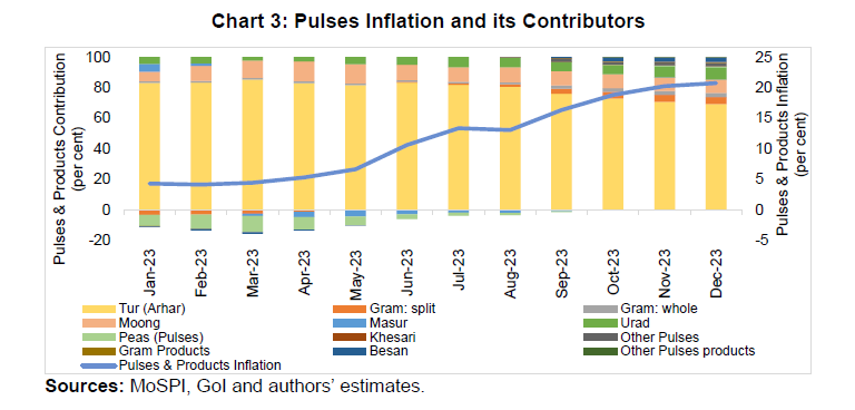

Typically, within a year, prices of a crop fall during the harvest time and begin to rise a few months before the arrival of the new crop (as the stocks plummet to their lowest at that time). Chart 4 shows seasonality factors in the CPI of the three selected pulses estimates using the U.S. Census Bureau’s X-13 seasonal adjustment procedures. The seasonality factors have been averaged over the last decade based on the crop year of gram, tur and moong. During the last decade, the CPI in gram whole has a trough around April, with the peak around November. In case of tur, CPI trough is around March; the prices increase around April to June with a slight stagnancy around June-July, before increasing further till October-November.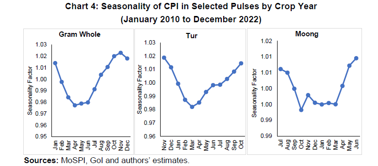

The moong crop is sown thrice a year, twice during kharif and once during rabi season. The kharif crop is sown during June to July and the rabi crop in September/October. The summer crop is sown during April. The harvesting of moong starts from August to December. Generally, moong CPI tends to trough around September to March. The prices begin to rise marginally thereafter, reaching peak levels in June, right before the start of the next crop.

IV.1Role of Government Supply Management Measures in Containing Pulses Inflation

Over the years, the government has undertaken a pro-active strategy to augment domestic supplies of pulses as well as to contain pulses inflation, which includes:

1. Incentives for by raising production under programmes like National Food Security Mission (NFSM);
2. Creating a buffer stock of pulses by undertaking procurement of different pulses, which is later offloaded into markets to contain price pressures;
3. Gradual liberalisation of import policy like bringing down applicable import tariff for some pulses, and bringing some pulses under open general licencing;
4. Invoking provisions of ECA like reporting of stock holdings, stock holding period, and imposing stocking limits on pulses from time to time; and
5. Signing Memorandum of Understanding (MoU) with countries which are sources of imports.

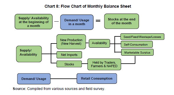
In addition, the Government has been making continuous efforts to give a boost to domestic production and achieve domestic self-sufficiency in pulses. In 2007-08, GoI launched the NFSM to increase acreage under pulses cultivation. The area under pulses increased from 23.6 million hectares to 25.8 million hectares between 2007-08 and 2023-24. India’s pulses production has risen consistently from 14.8 MMT in 2007- 08 to 23.4 MMT in 2023-24 (as per Second Advance Estimates), while that of gram rose from 5.7 MMT in 2007-08 to 12.1 MMT in 2023-24 and tur from 3.1 MMT to 3.3 MMT. For moong, production increased from 1.5 MMT to 3.7 MMT in 2022-23.¹⁴

The government also procures pulses at MSP and declares remunerative MSPs each year to incentivise farmers. As of 2023-24, moong had the highest MSP of Rs. 85.6 per kg, followed by tur’s MSP of Rs. 70 per kg, while gram had the lowest MSP at Rs.54.4 per kg (see Annexure A4 ). When prices of pulses rose sharply during 2015-16, the government decided to create a buffer stock of two million tonnes of pulses to be held by NAFED under the Price Stabilisation Fund (PSF) (MoCAFPD, 2016). NAFED carries out procurement of pulses from farmers through MSP operations for the creation of the buffer stock.¹⁵The government has increased the pulses buffer stocks target from 1.95 million tonnes in 2020-21 to 2.3 million tonnes in 2021-22 and 2022-23. NAFED procured pulses close to about 4.2 MMT in 2018-19 and 2.8 MMT in 2022-23 under the Price Stabilisation Scheme (PSS) (Chart 5 ). Provision for procurement of pulses above MSP has also been made in case need arises under the scheme of PSF. NAFED maintains this stock of pulses and on directions from the government, releases the stock in a calibrated manner, generally at below MSP, in the open market from time to time to moderate price volatility. For instance, to keep in check gram prices, in 2022 NAFED allocated 1.5 million tonnes of chana (gram) to the states at a discounted price of Rs. 8 per kg over the issue price for its distribution under various welfare schemes. More recently, the government launched sale of subsidised Chana Dal under the brand name ‘Bharat Dal’ for Rs. 60 per kg for a one kg pack and Rs. 55 per kg for a 30 kg pack in order to make pulses available to consumers at affordable prices by converting chana stock to chana dal.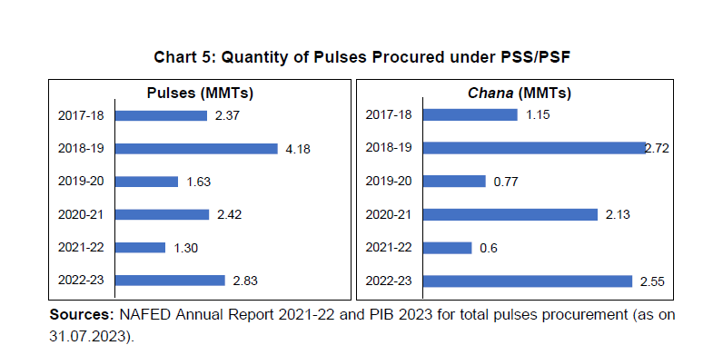

In order to prevent hoarding and check sharp spikes in pulses inflation, the government has been invoking the ECA and imposing stock limits on pulses from time to time. For instance, stocking limits were imposed on all pulses (200 MT for wholesalers and importers, and 5 MT for retailers) except for moong, under the ECA in July 2021. Likewise, in June 2023, the government imposed stock limits for tur and urad until 31st October 2023 to curb the rising inflation in the two pulses, which was further extended to 31st December 2023.

The government has, in the recent period, adopted various strategies to implement provisions of ECA like temporary requirement of weekly reporting in specific markets, time limit for holding stocks for importer and millers, calibrated reduction of effective import duties and freeing pulses import by bringing those under general open licencing among others.

IV.2. Trade Policy Instruments to Adjust Domestic Supply

As domestic production falls short of demand, the government stabilises supply and price pressures in pulses by manoeuvring the trade policy while ensuring continued remunerative prices for the farmers. The government uses a combination of trade policy tools as short-term instruments to augment supply and contain price inflation. These measures encompass (i) customs duties, (ii) minimum import prices (MIP), (iii) import quotas, (iv) import bans, and (v) export restrictions.

Prior to June 2017, pulses were imported on a zero-import duty structure, and there were export restrictions on pulses until 2015. Given the high dependence on imports and to protect the interests of farmers, the government increased import duty on pulses from 2017 onwards. For instance, the basic import duty was raised from zero per cent on all pulses to 10 per cent for tur in July 2017, and to 50 per cent for peas and 30 per cent for lentils and chickpeas in December 2017. However, import duty on moong and urad remained zero over the last decade (Chart 6 ).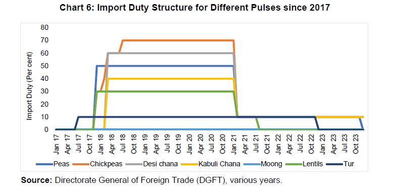

The import duties were further raised for chickpeas to 60 per cent in March 2018 and later to 70 per cent in July 2018. At the same time, a separate duty structure was introduced for kabuli chana and desi chana (Bengal gram), with import duties of 40 per cent and 60 per cent, respectively. India applies zero-duty imports for pulses imports from the least developed countries (LDCs) like Myanmar, Mozambique, Tanzania, Sudan, and Malawi.

Over time, the effective duty on tur was brought down from 10 per cent in March 2017, subject to a quantity restriction of 4 lakhs MT per fiscal year, to zero per cent import duty on tur whole in March 2023 to cater to domestic shortages. Moreover, the government extended the free import of tur till March 2025. Similarly, the import duty on kabuli chana and Bengal gram was brought down from 70 per cent in June 2018 to 10 per cent in February 2021. Since February 2021, Agriculture Infrastructure and Development Cess (AIDC) has been introduced and levied on the import of pulses, particularly peas (40 per cent), kabuli chana (30 per cent), Bengal gram (30 per cent), and lentils (10 per cent)16.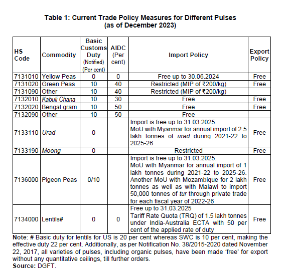

Table 1 illustrates import policy measures on different pulses as of December 2023. Given the high substitutability in pulses, the trade policy of competing pulses is calibrated to bring down pulses inflation. A classic example is the case of yellow peas. The magnitude of gram imports in a year is significantly affected by yellow pea imports as it can be used as a substitute for desi chana, particularly for the processing of gram flour (besan). Over the last decade, pea imports have been significantly higher than gram imports (See Annexure A5 )¹⁷. Due to lower import prices of yellow peas compared to domestic chana prices and to prevent pea imports from disrupting domestic market prices of chana, the imports of yellow peas were moved to the ‘restricted’ list from the ‘open’ category on April 25, 2018 (DGFT, 2018). Subsequently, the government effectively restricted imports of yellow peas by fixing a MIP of Rs. 200 per kg, which includes cost, insurance and freight (DGFT, 2019), and further did not allocate any import quota for yellow peas for 2020-21, 2021-22 and 2022-23 (DGFT, 2020). Prior to the restriction on the import of yellow peas, it was imported mostly from Canada, Australia, Russia and Ukraine. As per the discussions with the stakeholders in the pulses value chain, the imported price of yellow peas was in the range of Rs. 2000 to Rs. 2100 per quintal in 2018, while the MSP of gram or chana announced by the government was Rs. 4620 per quintal. Owing to such price disparities, the government adopted restrictive import policies like quantitative restriction (QR) and MIP on yellow peas to encourage gram production and improve domestic availability. However, on December 07, 2023, the government removed all the restrictions on yellow pea imports including the import duty, MIP, and port restrictions in a bid to contain high inflationary pressures and also because of expectations of lower chickpea production in the country (DGFT, 2023).

Apart from trade policy instruments, the government has entered into supply agreements (MoUs) with three countries – Myanmar, Mozambique and Malawi in June 2021. Under this agreement, India has made an annual commitment to import 2.5 lakh tonnes (urad) and one lakh tonne (tur) from Myanmar; 2 lakh tonnes (tur) from Mozambique; and 50,000 tonnes (tur) from Malawi during 2021-22 to 2025-26 (DGFT, 2021a and DGFT, 2021b).

V. Pulses Value Chain in India

The value chain of pulses (gram, tur and moong) can be explained by elaborating on the roles of various stakeholders (farmers, traders, processors and others) involved in the production, collection, packaging, transportation, processing, marketing and distribution of the produce to consumers (Chart 7 ). In the current value chain of pulses, small landholders usually grow pulses in rainfed conditions. The farmers produce these long-duration pulses variety keeping in mind weather vagaries and other external factors like demand and supply in the market for price realisation. Out of the total production, farmers generally keep a share of produce for self- consumption, seeds and feed, which ranges between 10-12 per cent for tur, gram and moong (DES, 2020). The rest of the quantity produced by the farmers has been considered as marketed surplus after deducting farm level wastages. The ICAR- CIPHET Report by Jha et al. (2015) estimated that the overall loss, i.e., losses in farm operations and storage, was 8.41 (±0.26) per cent in chickpeas, 6.36 (±0.30) per cent in pigeon peas, and 6.60 (±0.35) per cent in green gram. In the case of post-harvest losses, especially during milling and storage, traders state that losses have been reduced in recent years because of the creation of storage facilities at processor’s as well as wholesaler’s levels. Moreover, market intelligence and a discussion with the stakeholders in the pulses value chain indicated the proportion of conversion of the whole pulses by removing the husk and splitting the bean after processing into split dals, cattle feed, etc., for all the three pulses.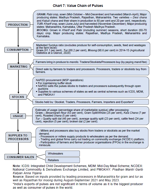

The processors of the commodity play a vital role in the marketing of the produce. The marketing channels of the raw pulses are carried out through mostly institutional and non-institutional channels from the producer to consumer. These channels consist of direct purchases from the farmers by traders and processors, commodities sold by the farmers to traders and processors at the mandis, and procurement operations carried out by the farmers’ cooperative NAFED. Institutional channels such as NAFED procure pulses for maintaining buffer stocks as well as for ensuring supplies for various state-specific social sector schemes. It also safeguards farmers when the mandi prices are below MSP. Although procurement through the cooperative network is not large in quantity, it helps protect farmers against price crashes.

Non-institutional channels consist of intermediaries, such as traders, wholesalers, commission agents, millers and retailers. Additionally, millers play an important role in the value chain of pulses since a major portion of these pulses is used in processed form (for example, besan in the case of chana) or as split pulses. After pulses enter the market, stockists, traders and processors also keep stocks of pulses, apart from the portion that farmers also keep aside before bringing to the market. This understanding of market fundamentals such as production, crop prospects, crop sowing pattern, imports and stocks held by the private sector and NAFED is important to bring stability in the prices of pulses.

Primary information collected from various mandis is used to understand how prices are formed in the case of pulses. We estimate the price mark-ups across all the three-value chains and estimate the share of farmers in a consumer’s rupee. As discussed earlier, supply chain dynamics and the contribution of mark-ups between farmgate and retail price are necessary to capture determinants of food inflation and its volatility. For estimating price mark-ups in the pulses value chain, the study has taken into account the prices prevailing in different mandis in Madhya Pradesh (for gram and moong) and Maharashtra (for tur).¹⁸In gram, around 75 per cent of the consumers’ rupee for chana goes back to farmers, while in moong and tur, it is about 70 per cent and 65 per cent, respectively as per our survey conducted in May 2023 (Table 2 ).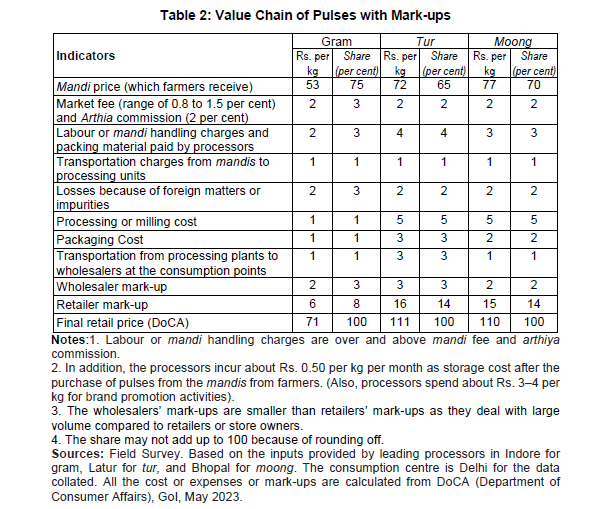

Within the pulses value chain, a major share of consumer rupee goes to the farmers, which highlights the efficiency of the pulses value chain. Apart from farmers, retailers also receive a large share of the consumer rupee. The reason is that retailers deal with smaller volumes and incur storage (display) costs at the sales points or outlets and thus have higher mark-up. In contrast, we observe that the processors’ mark-up has been relatively lower because of the large volume of trade they carry out throughout the year.

VI. Methodological Framework of Balance Sheet and Estimation

This section presents the methodological framework and balance sheet approach and how the monthly STU ratios have been constructed for the selected pulses.

VI.1. Balance Sheet Approach

The balance sheet approach has also been adopted by various organisations to track key agricultural commodities and explain movements in prices, such as the FAO under Agricultural Market Information System (AMIS), US Department of Agriculture’s Production, Supply and Distribution (USDA), and International Grain Council (IGC). Within India, several private agencies, like Agriwatch, monitor key agricultural commodities and use the balance sheet approach.

The current study, though built conceptually on existing approaches to constructing balance sheets for agricultural commodities, has gone beyond existing balance sheets in terms of scope, coverage and frequency. Unlike most existing balance sheets which are annual in frequency, the balance sheets constructed for gram, tur and moong in the study are monthly in frequency. While the balance sheet can be extended to a significantly long period in the past and into the future, attempts have also been made to account for seasonal pattern of production, market arrival, stocking and disposal, adjustment for population and income, and behavioural aspect of intermediaries in the value chain.

VI.1.1 Conceptual Framework of the Monthly Balance Sheet

The framework is based largely on official data on production, net imports, per capita consumption, income growth, and population. The study uses available secondary data sources, including GOI and state government websites and databases of state agriculture departments. For simplicity, an attempt has been made to use minimal assumptions based on information gathered from primary sources and existing academic literature. This, inter alia, pertains to deduction from available stocks allocated for seeds, feeds, wastages and losses, conversion rate between whole and grains, seasonal pattern of arrival and consumption, stocking and release patterns. These assumptions help in breaking down estimates of data which are provided in annual form into monthly frequency, as indicated in the flow chart given in Chart 8 .

The balance sheet can be extended for 12-months or more into the future, incorporating advance estimates. Likewise, the balance sheet can be extended back to the past subject to availability of relevant data. The balance sheet for the period ahead lends real-time utility and the information contained in the historical series, together, makes the balance sheet an ideal variable for price forecasting exercises. The monthly frequency renders significant value addition to the current balance sheet for use in empirical research and near to medium term assessment of the prospect of price pressures build-up. This is possible as the balance sheet already captures future availability, thereby facilitating knowing in advance the point when demand-supply mismatch could aggravate. Broadly, the dynamic monthly balance sheet is created to examine:

1. Supply and demand situation of the three pulses in the past, real time and near future;
2. Understand and evaluate the patterns involved – seasonal and behavioural - of harvest, arrivals, disposal by farmers, and of traders, importers, and consumers and incorporate them into the dynamic monthly balance sheet to understand how the market responds;
3. Since historical data on stocks is unavailable, we identify ways to measure monthly stock levels in the economy and, subsequently, compute STU ratios based on calculated total stocks;
4. Empirically examine the underlying patterns and trends of demand and supply under a structural framework, which is useful for understanding the price movements of the commodity; and
5. Use the balance sheets for short-term forecasting of the respective pulse’s inflation.

VI.1.2 Components of the Monthly Balance Sheet

In this sub-section, we first detail how the variables have been created, followed by an analysis of the estimated variable.

a. Supply Side: Net Availability Series Estimates

The gross availability of any pulses is defined as the sum of total production in the country and net imports.

From gross availability, we compute the net availability after deducting/ adjusting for seeds, feeds, self-consumption, and losses (at farm and storage level). Therefore, net availability is given as:

Here, the net production is basically:

With a view to keeping the model simple, minimal assumptions have been made. For instance, kharif and rabi pulses are assumed to have arrived or entered the supply chain in the months of December and April, respectively. It is also assumed that net production after adjusting for seeds, feeds, wastages, and losses is 90 per cent of gross or total production and the conversion ratio between whole and grains is 75:25, which is kept the same for all the pulses.¹⁹

b. Demand side: Cumulative Consumption Series Estimates

For computing the demand for pulses, we obtained the monthly per capita household consumption (MPCE) of pulses – both rural and urban, in volume terms as given by the NSSO quinquennial consumption and expenditure survey 2004-05 and 2011-12. Using the MPCE for two rounds, we computed the annualised monthly compounded growth rate of consumption between 2004-05 and 2011-12. We used the same monthly growth rate (the growth rate between NSSO CES 2004-05 and 2011- 12) for periods beyond 2011-12.²⁰Further, in order to arrive at monthly all-India rural and urban pulses consumption, the per capita monthly consumption series is multiplied with the monthly rural and urban population series, respectively. The weighted sum of rural and urban consumption series using the rural-urban population weight of 7:3 give all-India monthly total consumption of pulses.

The rural and urban series of monthly population is arrived at by applying annualised monthly compounded growth rate of population calculated using the 2001 and 2011 census population data of the Registrar General and Census Commissioner, India. In the absence of updated official census data, this computed growth rate of population has been applied for periods beyond 2011 as was done for MPCE. The population figure so arrived at is in close proximity of that arrived at by the United Nations for India.

Thereafter, the consumption series so obtained is adjusted with real growth rate of private final consumption expenditure (PFCE). This is done since there is no reliable estimate of monthly/quarterly/yearly income elasticity of demand for pulses. The real growth rate of PFCE, which is a quarterly series, is interpolated using standard splicing methodology to arrive at monthly PFCE series, in this case, Catmull-Rom-Spline has been used. This exercise renders consumption or demand to be dynamic that changes with per-capita income. Moreover, as Bennett's law observes, with a rise in income, people change their consumption patterns and consume relatively fewer calorie- dense, starchy staple foods and relatively more nutrient-dense meats, oils, sweeteners, fruits, and vegetables. Pulses being protein-dense, the Bennett’s Law is presumed to be applicable.

Finally, the monthly cumulative consumption series is arrived at by adding up monthly all-India consumption data of the current month with the preceding month/s starting January till December as below: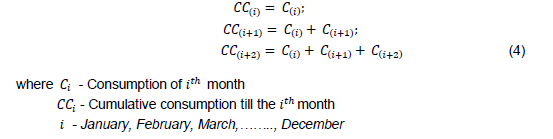

c.Stock Series Estimates

The total stock for each commodity, i.e., stock at the end of the 𝐴𝐴^𝑡𝑡ℎmonth is thus defined as :

d.Stock-to-Use (STU) Ratio Estimates

The STU ratio is an estimate of the level of carryover stocks for a given commodity at a point in time with respect to demand or usage. As such, the STU captures the interaction between demand and supply during the current month. The utility of STU ratio is, however, limited not only to assessing current month demand- supply pressure, but also the months ahead. In fact, it is the forward-looking information contained in STU ratios that is of essence for understanding the likely pressure that is going to get built-up going forward.

The formula for this relationship is as follows:

The higher the carryover stocks, the higher is the STU ratio and the lower demand-supply mismatch, and thus lesser the price pressure. A fair estimate of STU ratio should ideally serve as an important gauge for the likely future price pressure; therefore, it has to be an integral component of any model that forecasts prices. This is because, in essence, STU ratios capture how much of the current need is met from available stock and how much is available for meeting future consumption needs.

The three STU ratios so calculated using the methodology elaborated above for the pulses under study are given in Table 3 . In line with economic theory, the respective estimated STU ratios have a negative relationship with the respective prices, with varying degrees of correlations. The differing correlation coefficient for the pulses may be attributed to a host of factors, namely, extent of scarcity or sufficiency of the pulses – production level and flow of imports, role of millers and traders or the market dynamics, efficiency of price discovery mechanism, and prevailing intervention policies of the government, among others. For instance, the negative but a lower correlation coefficient for tur – the relatively scarce and more price sensitive pulses compared with gram which has sufficient domestic supply – may be indicating that other factors rather than only STU ratio are at play in determining prices. Similarly, moong – costlier, traded more and available abundant, yet, consumed in lesser quantity or less a staple – was found to have negative but low correlation coefficient. Gram, the more relatively abundant and self-reliant with the largest share in domestic production and consumption, has the strongest correlation between its STU and price.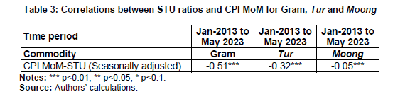

VI.2. Model Specification

In line with the objectives, firstly, the study identifies various demand and supply determinants of prices for gram, tur and moong in an ARDL framework. As the variables utilised to define factors in pulses regression may exhibit different levels of integration, the ARDL cointegration technique is used as it is suited for scenarios where the variables have different orders of integration. This method is robust when dealing with cases where a solitary long-term relationship exists between the fundamental variables, especially, when the available sample size is small (Pesaran and Shin, 1999; and Pesaran et al., 2001).

The ARDL model adopts a single-equation framework. This allows it to incorporate an appropriate number of lags and effectively guide the data generating process within a framework that transitions from general to specific modelling. To illustrate the ARDL modelling approach, a general ARDL(p, q) model is given by:

The error correction model (ECM) version of the ARDL is given by:

where, ∆ is the first difference operator, 𝑃𝑃0 is the constant; 𝑌𝑌𝑡𝑡 is the CPI of specific pulses items expressed in log terms, 𝑋𝑋𝑖𝑖 are the ‘k’ explanatory variables, 𝑃𝑃𝑡𝑡 is the white noise error term, 𝐼𝐼 and 𝑞𝑞 (which could be different across the ‘k’ explanatory variables) are the optimal lag lengths. The optimal lag length has been obtained using Akaike Information Criterion (AIC). All the coefficients are non-zero. ECMt-1 (𝜀𝜀̂𝑡𝑡−1) is the error correction term which measures the deviations from long-run equilibrium relationship, and the ECM coefficient 𝛾𝛾 denotes the speed of adjustment of the dependent variable towards the long run equilibrium relationship following any short-run deviation due to shocks within a period. The ECM coefficient (𝛾𝛾) is expected to be negative (𝛾𝛾 < 0) and statistically significant. The ECM integrates the short-run dynamics with the long-run equilibrium without losing long-run information and avoids problems such as spurious relationship resulting from non-stationary time series data.

The ARDL method provides unbiased estimates and valid t-statistics, irrespective of the endogeneity of some regressors (Harris and Sollis, 2003 and Jalil and Ma, 2008). As far as the short-run adjustments are concerned, they can be integrated with the long-run equilibrium through the ECM. The bounds test (Pesaran et al., 2001) is used to test for the presence of long run cointegration.

The dependent variables, log of CPI gram, tur and moong, are specified using the seasonally adjusted log of CPI (log_𝐶𝑃𝐼𝑡), while the explanatory variables include stock to use raios (STU𝑡_Pulse_𝑆𝐴), proxy for market dynamics (Mark) which is thdifference between 𝐶𝑃𝐼𝑡_Pulse_MoM and the margin between retail and wholesale price momentums. The information contained in this Mark variable, which is available one-and-half months in advance before the actual CPI print, has a significant lead indicator value and is an important gauge for emerging price pressures. Since the Mark variable is deviation of margin from actual momentum, the variable can be assumed to reflect market sentiment. The Pulse_𝐷ummy captures the impact of lean season as well as the COVID-19 pandemic induced lockdowns on pulses prices. Seasonality is a dominant feature of fluctuations in food prices, and therefore, the U.S. Census Bureau’s X-13 seasonal adjustment procedures in EVIEWS has been used for seasonal adjustment.

VI.2.1 Estimations and Results of the Drivers of Gram, Tur and Moong Prices

Gram Estimation

Before applying the ARDL, stationarity check was done for all the variables using Augmented Dickey-Fuller (ADF) test. The results show that the included variables are stationary in first differences (Table 4 ).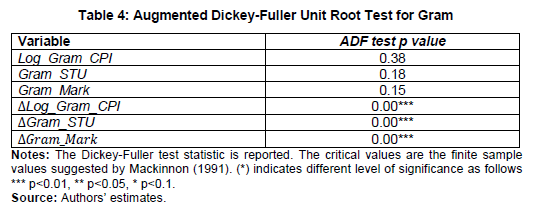

The lag lengths are chosen using the AIC criterion, which leads to ARDL (2,1,4,4) model. The ARDL bounds test confirms the presence of a cointegrating relationship between Gram_CPI, stock-to-use of gram, Gram mark and Gram dummy (Table 5 ).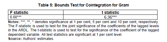

The estimates of long-run coefficients from ARDL specification and the short run dynamics are presented in Table 6 . The coefficient of Gram_STU is negative and significant. This is in line with the hypothesis of this study that stock helps control price pressure - higher the stock, lower the prices. The supply chain disruptions and seasonal impact, particularly, COVID-19 captured by Gram_Dummy, did contribute to the price pressure. There was perceptible movement in the price of gram during COVID-19 despite Gram being one of the most stable pulses in terms of price volatility. These observations are amenable to ground realities as regards gram, which is relatively more comfortable in supply, constituting around 50 per cent of total production. The statistically significant and negative coefficient of the ECM term indicates that any deviation from the long run equilibrium will take a long time to correct.

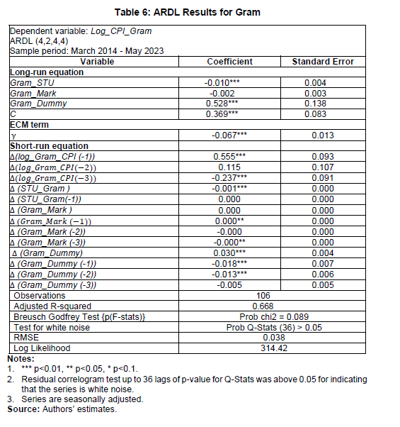The diagnostic tests are satisfactory: the error term is white noise, i.e., independent and identically distributed with homoskedasticity and normality. The Breusch-Godfrey test indicates that there is no serial correlation (at 1 or 5 per cent level of significance). The CUSUM test shows that the errors remain within the 95 per cent confidence band suggesting that the estimated model is stable (Chart 9 ).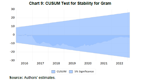

Tur Estimation

The ADF unit root tests indicate that CPI tur, CPI-besan and Tur_STU are stationary in first differences and Tur_Mark is stationary in level (Table 7 ).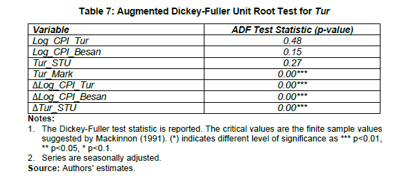

The ARDL bounds test confirms the presence of a long-run cointegrating relationship between Log_CPI_Tur, STU, Tur_Mark, Dummy and Log_CPI_Besan (Table 8 ). The selected ARDL model is (2,0,0,4,4).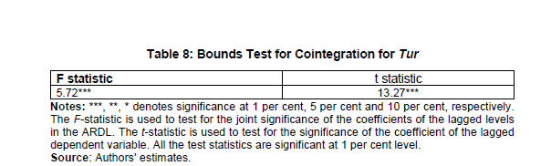

The estimates of long-run coefficients and the ECM are represented in Table 9. The coefficient of Tur_STU was negative but statistically insignificant. In case of tur, domestic production is not sufficient to meet consumption requirement and there are limited sources for import, namely, Myanmar and few African countries. Tur being the scarcest of all pulses exhibits the most volatile price behaviour. This has been reinforced by the positive and significant coefficient of Tur_Mark confirming that margins and sentiments amplify tur prices. The price of besan (which is processed from gram), showed a strong statistical relationship – both in short and long-run, indicating that substitution of tur by besan was effective and taking place continuously. The model also captures the impact of seasonal – tur is a kharif crop cultivated once a year unlike other double or multi crop pulses – and supply chain disruption during COVID-19. The interplay of these dynamics resulted in a low speed of adjustment as captured by the coefficient of ECM term indicating that any deviation from the long-run equilibrium will take long time to correct.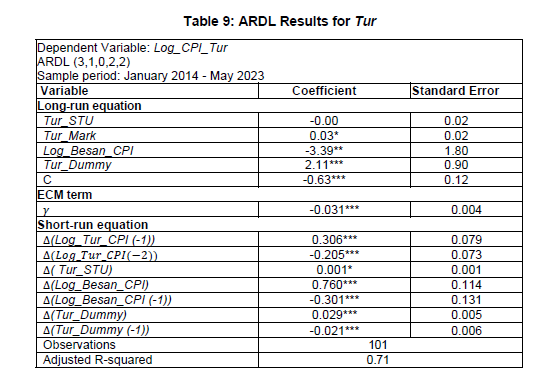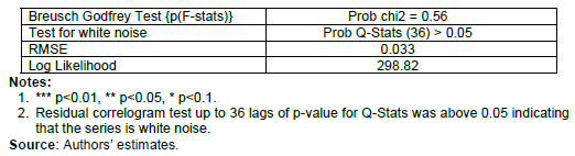

The diagnostic tests are satisfactory: the error term is white noise, and the model is stable as indicated by cumulative sum (CUSUM) test (Chart 10 ).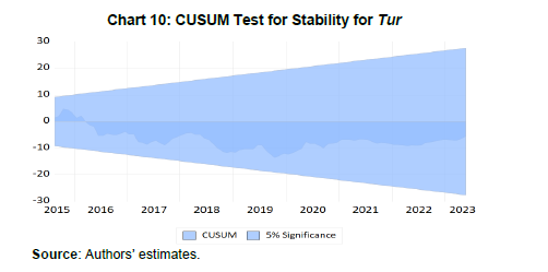

Moong Estimation

In case of moong, the ADF unit root test shows that the included variables are stationary in first differences (Table 10 ).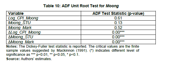

The ARDL bounds test confirms the presence of long-run cointegrating relationship between log_CPI_Moong,STU,Mark and the Dummy (Table 11 ).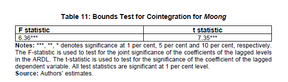

The estimates of long-run coefficients from the ARDL specification and the short run dynamics are presented in Table 12 . Despite being adequate in domestic supply and per capita consumption lower than other pulses, moong is actively traded since it is costlier. Like in other pulses, margin and market sentiments captured by Moong_Mark amplifies price pressures in Moong. The model also captures the impact of seasonal and COVID-19 supply disruption on Moong prices in the short- and long- run. The statistically significant and negative coefficient of ECM term indicates that any deviation from the long run equilibrium will take a long time to correct.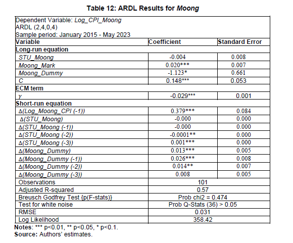

The diagnostic tests for the ARDL model are satisfactory and the model is stable as per the CUSUM test (Chart 11 ).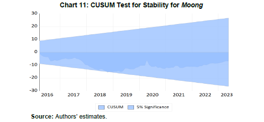

VI.3. Inflation Forecasts for Gram, Tur and Moong

Various studies have been undertaken to better understand and forecast food inflation in the Indian context (Sonna et al., 2014 and Raj et al., 2019). For forecasting inflation, the empirical literature has used a number of individual models such as seasonal autoregressive integrated moving average (SARIMA) models, SARIMA with exogenous variable (SARIMA-X), ARMA, random walk (RW) model, autoregressive (AR) model, moving average model (MA), vector autoregression (VAR) models, VAR with exogenous variables (VAR-X), models with Generalised Autoregressive Conditional Heteroscedasticity (GARCH) and Phillips curve (John et al., 2020; Stock and Watson, 2009; Benes et al., 2016; Aiolfi and Timmerman, 2006 and Behera et al., 2018). However, no individual model - univariate or multivariate – is superior in accurately forecasting inflation. Stock and Watson (2009) suggested that in comparison to the parsimonious forecasting techniques, models with a large number of predictors tend to fare poorly. The empirical study by Bhattacharya et al. (2019) on forecasting inflation highlighted that a simple time-series estimation model supplemented with an exogenous variable could improve the forecast performance of the model.

As observed in the literature, while models like ARDL capture well the price dynamics, they do not necessarily perform better in forecasting. The same was also observed in this study. Accordingly, following the literature, the present study uses univariate time series models while introducing some important balance sheet variable and market variable identified in the structural model, mainly STU and Mark, to improve short-term forecasting. We attempt to forecast inflation for gram, tur, and moong for a 12-month horizon using time series-based univariate and multivariate models such as:

1. SARIMA: SARIMA model based on its own past values and the lagged forecast errors is used to forecast future pulses inflation, assuming that the time series has a constant variance of errors (homoscedasticity) (Gujarati and Sangeeta, 2007).
2. SARIMAX: In addition to modelling the dependent variable solely as a function of its past values and disturbances under the discussed SARIMA models, we have also used SARIMAX modelling, where the dependent variable is studied as a linear combination of more than one independent variable (STU and Mark in our case), as well as an ARMA disturbance process (StataCorp, 2023).

The present paper explores these two univariate and multivariate forecasting techniques to provide 12-month horizon prediction for each of the selected pulses (gram, tur and moong). This will be helpful to check if the robustness of forecast performance improves while using the balance sheet variables: STU ratio (SARIMAX) or if past error terms are providing better forecast (SARIMA). As the variables used in the forecasting analysis are integrated of different order, the non-stationary variables were transformed using the first difference transformation to make them stationary.

VI.3.1 Empirical Analysis of Forecasts

Using pseudo out-of-sample root mean squared error (RMSE) of individual models and multivariate models, we evaluated the performance and accuracy of various inflation forecasting techniques for horizons of up to 12 months ahead. The evaluation was done by stopping the full sample period in February 2022 and generating forecasts for 2, 4, 6, 8, 10, and 12 months until February 2023, which were then compared with actual inflation of these pulses.

The RMSEs of each forecasting model were evaluated using both in-sample and out-of-sample forecasts for the full sample period (i.e., January 2014 to February 2023). This gives a measure to evaluate model’s accuracy in a historical time frame. Further, we also evaluate the accuracy of the pseudo out of sample forecasts up to 12 months ahead, generated between February 2022 and February 2023, which gives an overview of the range of forecast errors in one year ahead period. The evaluation of RMSE of univariate and multivariate model forecasts for gram, tur and moong is given in TTable 13 .

For gram, the SARIMAX forecasts outperform SARIMA across all the forecast horizons in the ‘Full sample’ and in the ‘Out-of-sample’ forecasts evaluation. The exogenous variable used in SARIMAX forecasting for gram include seasonally adjusted STU of gram (STU) and gram mark (which captures the market dynamics).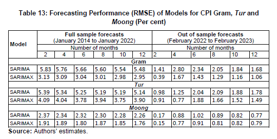

In tur, similarly, SARIMAX model outperforms all other models over each horizon in ‘Full sample’ and in the ‘out of sample’ forecasts evaluation. For forecasting SARIMAX of tur, the exogenous variables used are seasonally adjusted STU, Mark and BesanCPI.

In the case of moong, SARIMAX outperforms SARIMA in the ‘Full sample forecast evaluation’ across all forecast horizons, and in the ‘Out of sample forecast evaluation’ except at 10- and 12-months horizons. For forecasting SARIMAX of moong, the exogenous variables used are seasonally adjusted STU and Mark. Annexure A6 and A7 provide the forecast results of gram, tur and moong.

These observations support the study’s hypothesis that the balance sheet variable (stock or STU ratio) along with other variables like market dynamics can improve forecasting performance of inflation in gram, tur and moong.

VII. Conclusion and Policy Suggestions

Volatility in inflation of pulses over the last decade has been a concern for policymakers. In periods of sharp increase in pulses prices such as 2015-16 and 2016- 17, as well as the post-pandemic period, the government has taken various supply management measures, such as de-regulating trade policy instruments, incentivising production and creating a buffer stock of pulses by NAFED, to boost domestic supplies and contain inflation. Select provisions of the Essential Commodities Act (ECA) have also been applied in recent period albeit sparingly in a more transparent and targeted manner. There is unanimity that though the country is still not fully self-reliant in pulses production, large fluctuations in prices of pulses could adversely affect consumption and the supply gaps can be tackled to a large extent with better policy response.

The present study creates a dynamic monthly balance sheet to evaluate the demand-supply gap of each of these pulses on a real-time basis and computes the STU ratio of the selected pulses using inputs provided by key stakeholders such as farmers, traders and processors in the pulses value chain and the official data. The hypothesis is that STU helps explain prices better in each of these pulses after controlling for other demand and supply-side factors. Estimates using ARDL framework indicate that STU ratio in case of gram and market dynamics (captured by the Mark variable) in case of tur and moong, among others have important bearings on their prices. Further, incorporation of these variables in multivariate framework under SARIMAX set-up aided in improving forecasting accuracy of pulses inflation.

Lastly, based on the findings, the study suggests several policy measures for stabilising pulses prices as set out below.

Short-run Measures: Rationalising Trade Policy for Containing Inflation in Pulses

A prudent policy to moderate and stabilise pulses inflation could be by modulating the trade policy through timely calibration in applicable duties. During domestic shortages, a liberal and consistent trade policy could help importers plan appropriately, thereby helping contain surge in prices. By adjusting import duties proactively, the domestic supply-demand gap could be addressed effectively. Similarly, during periods of surplus production when prices plummet, trade policies could be dynamic to respond to market conditions effectively, thereby averting price crashes. Moreover, the opportunity to fetch better prices in the global market could encourage farmers to upgrade productivity.

Additionally, minimum export prices and transparent export duties may effectively manage exports in the short-term. Some of these measures were introduced recently to contain pulses inflation.

Long-term Measures: Improving Productivity and Production through Innovations

For the country to achieve self-sufficiency in pulses, it is imperative to invest in long-run agricultural productivity and production growth in pulses along with infrastructural investments, such as warehouses and efficient storage facilities that can enhance supply responses. There is a need to consolidate production at the farmers’ levels through FPOs or any collectives so that farmers can realise better prices for their produce and, thereby, incentivised to use modern agricultural inputs and technology.

Reduction in pre- and post-harvest losses of farmers would improve their price realisation. At the same time, processing losses can be reduced through better varietal development. Notably, distributing seed storage bins to farmers and increasing

awareness about adoption of scientific methods of storage of pulses at the farm level through agricultural extension services can significantly reduce losses at the storage level.

Also, additional emphasis is needed for varietal development to suit the local agro-climatic conditions that are climate resilient and are of short-duration. For instance, the traditional varieties of tur seeds, such as Laxmi, Bahar, Gwalior 3 and C11, sown in rainfed conditions, require around 180 days for maturity. However, the Indian Council for Agricultural Research’s (ICAR’s) new short-duration variety, Pusa Arhar-16, has reduced the maturity period to around 120 days while increasing yield by around 15 per cent compared to the traditional varieties. There is a need to introduce new seed varieties for gram, moong and other pulses for large- scale commercial cultivation so that farmers’ remuneration could get a boost because of the short crop duration and higher yield of the tur variety.

Enhancing Efficiency in Marketing System and Value Chain

The access to an efficient marketing system and strengthening the fragmented and weak supply line can facilitate better price discovery and transparency. It can address price fluctuation in pulses in a number of ways:

First, the integration of the Electronic-National Agriculture Market (e-NAM), especially in key producing regions of pulses, may bring much-needed transparency to the pulses trade. Improving the grading facilities at the mandis as envisaged under e-NAM would help processors access quality and graded produce at the mandi level, thus improving the efficiency of the value chain. For instance, some APMC mandis in Andhra Pradesh, Telangana and Karnataka have initiated trading of pulses.

Second, as most of the farmers producing pulses belong to the small holder category, they depend on the mandi system for marketing their produce. The direct purchases by processors from the aggregator/FPOs/farmer at the farmgate level would reduce transportation costs to bring the produce to mandis as well as provide bargaining power to the farmers. Under the current system, farmers bring in their produce to mandis and sell their produce to traders as well as processors while incurring the cost of transactions (mandis and arthia or commission agents’ fees). Additionally, the direct purchase would help cut down on intermediaries and reduce transaction costs, which would provide benefits to farmers as well as the traders and processors.

Third, at the processing level, more technological interventions are needed to improve the conversion ratio of whole pulses into split or processed dal or pulses products. The processing of pulses is mostly done in the private sector; therefore,

installing small pulses mills or processing units at the village level can reduce the cost of processing as has been highlighted in the literature.

Fourth, there is a need to scale-up and operationalise procurement of pulses – domestic and import - in quantities sufficient for market intervention and maintaining strategic buffer reserves. Government procurement and disbursal from NAFED stock and strategic buffer have helped contain inflation in the recent past. The scheme may have to assume a greater role and acquire increased efficiency to ensure stability in pulses prices given the seasonality of supply - lean and glut, and the continuing inadequacy of domestic supply in meeting domestic requirements fully.

References

Abraham, M., & Pingali, P. (2021). Shortage of pulses in India: Understanding how markets incentivize supply response. Journal of Agribusiness in Developing and Emerging Economies, 11(4), 411–434. https://doi.org/10.1108/JADEE-11-2017-0128

Aiolfi, M., & Timmermann, A. (2006). Persistence in forecasting performance and conditional combination strategies. Journal of Econometrics, 135(1-2), 31-53.

AMIS. Agricultural marketing information system. https://www.amis- outlook.org/index.php?id=40182

Anand, R., Ding, D. & Tulin, V. (2014). Food inflation in India: The role for monetary policy. IMF Working Paper No. 14/78, IMF. https://ssrn.com/abstract=2519004

Anand, R., Prasad, E.S., & Zhang, B. (2015). What measure of inflation should a developing country central bank target? Journal of Monetary Economics, 74, 102– 116.

Aoki, K. (2001). Optimal monetary policy responses to relative-price changes. Journal of Monetary Economics, 48 (1), 55-80. https://doi.org/10.1016/S0304-3932(01)00069-1.

Banerjee, A., Dolado, J., & Mestre, R. (1998). Error‐correction mechanism tests for cointegration in a single‐equation framework. Journal of Time Series Analysis, 19(3), 267-283.

Banerji, A., & Meenakshi, J. V. (2004). Buyer collusion and efficiency of government intervention in wheat markets in northern India: an asymmetric structural auctions analysis. American Journal of Agricultural Economics, 86(1), 236–253. http://www.jstor.org/stable/3697887

Behera, H., Wahi, G., & Kapur, M. (2018). Phillips curve relationship in an emerging economy: Evidence from India. Economic Analysis and Policy, 59 (C), 116-126.

Benes, J., Clinton, K., George, A.T., Gupta, P., John, J., Kamenik, O., Laxton, D., Mitra, P., Nadhanael, G.V., Portillo, R., Wang, H. & Zhang, F. (2016). Quarterly projection model for India: Key elements and properties. RBI Working Paper, 08/2016 (RBI WPS (DEPR): 08/2016). Department of Economic and Policy Research. Reserve Bank of India, Mumbai https://rbidocs.rbi.org.in/rdocs/Publications/PDFs/WPSN8EC0A00B61AC2462797F9C1DDCCBB5078.PDF

Bhalla, S.S., Choudhary, A., & Mohan, N. (2011). Indian inflation: populism, politics and procurement prices. Developing Trends: Oxus Research Report.

Bhattacharya, R. (2016). How does supply chain distortion affect food inflation in India? NIPFP Working Paper Series, No. 173. New Delhi: National Institute of Public Finance and Policy.

Bhattacharya, R., & Jain, R. (2020). Can monetary policy stabilise food inflation? Evidence from Advanced and Emerging Economies. Economic Modelling, 89, 122- 141.

Bhattacharya, R., Jain, R., & A. Singh. (2019). Measuring the contribution of mark-up shock in food inflation in India. IIMB Management Review, 31(2), 167-181, https://doi.org/10.1016/j.iimb.2019.03.015.

Bhattacharya, R., & Sengupta, A. (2015). Food inflation in India: Causes and consequences. NIPFP Working Paper 2015/151. National Institute of Public Finance and Policy, New Delhi.

Bhoi, B. B., Kundu, S. Kishore, V. & Suganthi D. (2019). Supply chain dynamics and food inflation in India. RBI Bulletin, October. Department of Economic Policy and Research, Reserve Bank of India.

Bhattacharya, R., & Sengupta, A. (2018). Drivers and impact of food inflation in India, Macroeconomics and Finance in Emerging Market Economies, 11(2), 146-168. DOI: 10.1080/17520843.2017.1351461

Catao, L.A., & Chang, R. (2015). World food prices and monetary policy. Journal of Monetary Economics 75, 69–88.

Dawe, D. (2009). The unimportance of “low” world grain stocks for recent world price increases. Agricultural and Development Economics Division (ESA) Working Paper 09-01, Food and Agricultural Organization, Rome. www.fao.org/es/esa/en/pubs_wp.htm

Deaton, A., & Laroque, G. (1992). On the behaviour of commodity prices. The Review of Economic Studies, 59(1), 1–23. https://doi.org/10.2307/2297923

DES (2020). Agricultural statistics at a glance 2020. Directorate of Economics and Statistics, Ministry of Agriculture and Farmers Welfare, Government of India. https://agriwelfare.gov.in/Documents/CWWGDATA/Agricultural_Statistics_at_a_ Glance_2020_0.pdf

DES (2022). Agricultural statistics at a glance 2022. Directorate of Economics and Statistics, Ministry of Agriculture and Farmers Welfare, Government of India. https://agriwelfare.gov.in/Documents/CWWGDATA/Agricultural_Statistics_at_a_ Glance_2022_0.pdf

DES (2024). Second advance estimates of production of foodgrains for 2023-24. Directorate of Economics and Statistics, Ministry of Agriculture and Farmers Welfare, Government of India. https://desagri.gov.in/wp- content/uploads/2023/11/Time-Series-Production-of-First-AE-2023-24-1.pdf

DGFT (2018). Notification No. 04/2015-2020, April. Ministry of Commerce and Industry, Directorate General of Foreign Trade, Government of India. https://content.dgft.gov.in/Website/04 eng.pdf

DGFT (2019). Notification No. 37/2015-2020, December. Ministry of Commerce and Industry, Directorate General of Foreign Trade, Government of India. https://content.dgft.gov.in/Website/37%20english_1.pdf

DGFT (2020). Notification No. 04/2015-2020, April. Ministry of Commerce and Industry, Directorate General of Foreign Trade, Government of India. https://content.dgft.gov.in/Website/Trade%20Notice%20No%2004.pdf

DGFT (2021a). Notification No. 09/2015-2020, June. Ministry of Commerce and Industry, Directorate General of Foreign Trade, Government of India. https://content.dgft.gov.in/Website/dgftprod/b217d403-d544-4e41-bd27- ef8aea81cbaf/PN%209%20dt%2024-06-21%20Eng.pdf

DGFT (2021b). Notification No. 44/2015-2020, March. Ministry of Commerce and Industry, Directorate General of Foreign Trade, Government of India. https://content.dgft.gov.in/Website/dgftprod/2e1205c0-0b75-488a-aa84- 8017f7ac4664/PN%2044%20English%20pdf.pdf

DGFT (2023). Notification No. 50/2023, December. Ministry of Commerce and Industry, Directorate General of Foreign Trade, Government of India. https://content.dgft.gov.in/Website/dgftprod/75102910-8c8f-4e02-b313- e082b949bae3/Notification%2050%20dt%2008-12-23%20Eng.pdf

FAOSTAT. FAOSTAT (Food and Agriculture Data). https://www.fao.org/faostat/en/#data/TCL

Food and Agricultural Organisation (FAO). The Food and Agriculture Organisation Database. http://www.fao.org/statistics/en/

Ganguly, K. & Gulati, A. (2013). The political economy of food price policy – the case of India. WIDER Working Paper, No. 2013/034, The United Nations University World Institute for Development Economics Research (UNU-WIDER), Helsinki

Gokarn, S. (2011). Food inflation: This time it’s different. RBI Monthly Bulletin, January, Reserve Bank of India.

Gopakumar K., & Pandit V. (2017). Food inflation in India: Protein products. Indian Economic Review, 52(1/2), 157-179.

Gujarati, D. & Sangeetha, N. (2007). Basic econometrics. Fourth Edition, Tata McGraw-Hill, New Delhi.

Gulati, A., & Saini, S. (2013). Taming food inflation in India. Discussion Paper No. 4, Commission for agricultural costs and prices, Ministry of Agriculture, Government of India.

Gulati, A., Jain, S., & Satija, N. (2013). Rising farm wages in India: The ‘pull’ and ‘push’ factors”. Discussion Paper No. 5. Commission for Agricultural Costs and Prices, Ministry of Agriculture, Government of India. https://doi.org/10.1016/j.jmoneco.2015.06.006

Gustafson, R. (1958). Carryover levels for grains, USDA, Technical Bulletin 1178:

Washington DC.

Harris, R., & Sollis, R. (2003). Applied time series modelling and forecasting.

Hoboken, NJ: John Wiley and Sons.

IGC. International grains council. https://www.igc.int/en/markets/marketinfo-sd.aspx.

Jalil, A., & Ma, Y. (2008). Financial development and economic growth: Time series evidence from Pakistan and China. Journal of Economic Cooperation Among Islamic Countries. 29(2), 29-68

Jha, S., Vishwakarma, R., Ahmad, T., Rai, A., & Dixit, A. K. (2016). Assessment of quantitative harvest and post-harvest losses of major crops and commodities in India. ICAR-All India Coordinated Research Project on Post-Harvest Technology, ICAR-CIPHET, PAU, Ludhiana. DOI: 10.13140/RG.2.1.3024.3924.

John, J., Singh, S., & Kapur, M. (2020). Inflation forecast combinations - the Indian experience. RBI Working Paper Series No 11, (RBI WPS (DEPR): 11/2020). Department of Economic and Policy Research. Reserve Bank of India, Mumbai

John A.T., Makkar, S., Swaminathan, S., Minocha, S., & Webb, P. (2021). Factors influencing household pulses consumption in India: a multilevel model analysis. Global Food Security. https://doi.org/10.1016/j.gfs.2021.100534.

Joshi, D., Deshpande, D., Tandon, P., & Parambalathu, K. (2017). Pulses and rhythms: Analysing volatility, cyclicality and the cobweb phenomenon in prices. CRISIL, 11 September. www.crisil.com/content/dam/crisil/ouranalysis/reports/Research/CRISIL- Research-Report-Pulses-and-Rhythms-11Sept2017.pdf.

Kapur, M., & Behera, H. (2012). Monetary transmission mechanism in India: a quarterly model. RBI Working Paper No. 09/2012 (RBI WPS (DEPR): 09/2012). Department of Economic and Policy Research. Reserve Bank of India, Mumbai

Kumar, P. (2017). Food and nutrition security in India: the way forward. Agricultural Economics Research Review, 30 (1). DOI:10.22004/ag.econ.263546

MacKinnon, J. (1991). Critical values for cointegration tests. In: Engle, R. and Granger, C., Eds., Long-run Economic Relationships, Oxford University Press, Oxford, 267- 276.

Ministry of Statistics and Programme Implementation (MoSPI) and World Food Programme (WFP). (2019). Food and nutrition security analysis, India, 2019. Governmentof India. https://www.mospi.gov.in/sites/default/files/publication_reports/document%281%29.pdf

MoCAFPD (2016). Price Stabilisation Fund. Department of Consumer Affairs. Government of India. https://consumeraffairs.nic.in/sites/default/files/file- uploads/price_monitoring/PSF%20Operational%20Guidellines%20DOCA_0.pdf

Mohanty, D. (2014). Why is recent food inflation in India so persistent? Speech delivered at the annual Lalit Doshi Memorial Lecture, Xavier’s Chapter, delivered at the St. Xavier’s College, Mumbai.

Mohanty, S., & Satyasai, K.J. (2015). Feeling the pulses - Indian pulses sector.

NARARD Rural Pulse. Issue 10, July-August, Department of Economic Analysis and Research, National Bank for Agriculture and Rural Development. https://www.nabard.org/auth/writereaddata/tender/2009164501Rural-Pulse-July- August-2015.pdf

Nair, S. R. & Eapen, L.M. (2012). Food price inflation in India (2008 to 2010): A Commodity-wise analysis of the causal factors. Economic and Political Weekly, 47(20), 46-64.

Nair, S. R. & Eapen, L.M. (2015). Agrarian performance and food price inflation in India: Pre- and post-economic liberalisation. Economic and Political Weekly, l(31), 49-60.

Narayanan, S. (2022). How India’s agrifood supply chains fared during the COVID-19 lockdown, from farm to fork. (Ed.) McDermott, J. and Swinnen, J., COVID-19 and Global Food Security. The International Food Policy Research Institute.

Nerlove, M. (1958). The dynamics of supply: estimation of farmers’ response to price.

Johns Hopkins University Press: Baltimore.

GoI (2012). National sample survey 2011-2012 (68th round) (Type 1) – Household Consumer Expenditure. Ministry of Statistics and Programme Implementation, Government of India, New Delhi.

Pesaran, M.H., & Shin, Y. (1999). An autoregressive distributed lag modelling approach to cointegration analysis. In: Strom, S., Ed., Chapter 11 in Econometrics and Economic Theory in the 20th Century, The Ragnar Frisch Centennial Symposium, Cambridge University Press, Cambridge, 371-413. https://doi.org/10.1017/CCOL521633230.011

Pesaran, M.H., Shin, Y. & Smith, R. (2001). Bounds testing approaches to the analysis of level relationships. Journal of Applied Econometrics, 16(3), 289-326. https://doi.org/10.1002/jae.616

Raj, J., Kapur, M., Das, P., George, A.T., Wahi, G., & Kumar, P. (2019). Inflation forecasts: recent experience in India and a cross-country assessment. Mint Street Memo No. 19, Reserve Bank of India.

Rampal, P. (2017). Situational analysis of pulse production and consumption in India,

LANSA Working Paper Vol 2017 No 20. Bighton. IDS

Rangarajan, C., & Sheel, A. (2013). Relevance of Keynesianism in the post-recession period. Economic and Political Weekly, 48(33),32–39. http://www.jstor.org/stable/23528087

Reserve Bank of India. (2018). Annual Report 2017–2018. Reserve Bank of India. Roache, S. K. (2010). What explains the rise in food price volatility? IMF Working

Papers 10/129, International Monetary Fund.

Samuelson, P. (1971). Stochastic speculative price. Proceedings of the national academy of sciences, Vol. 68, pp 335–337.

SANDRP. (2015). Pulses farmers: custodians of fertility, water and climate-friendly agriculture. https://sandrp.in/2015/10/20/pulse-farmers-custodians-of-fertility- water-and-climate-friendly- agriculture/#:~:text=Water%3A%20First%20of%20all%2C%20pulses,about%202 0%20times%20less%20water.

Sekhar, C.S.C., Roy, D., & Bhatt, Y. (2018). Food inflation and volatility in India: trends and determinants. Indian Economic Review, 53 (1/2), 65-91. https://doi.org/1 0.1 007/s41 775-01 8-001 7-z

Sonna, T., Joshi, H., Sebastian, A., & Sharma, U. (2014). Analytics of food inflation in India. RBI Working Paper Series No. 10 (RBI WPS (DEPR): 10/2014). Department of Economic and Policy Research. Reserve Bank of India, Mumbai. https://rbi.org.in/Scripts/PublicationsView.aspx?id=16055

StataCorp. 2023. Stata Statistical Software: Release 18. College Station, TX: StataCorp LLC. https://www.stata.com/features/time-series/ts-arima.pdf

Stigler, M & Prakash, A. (2011). The role of low stocks in generating volatility and panic, in Adam Prakash (ed.) Safeguarding Food Security in Volatile Global Markets. FAO: Rome.

Stock, J. M., & Watson, W. (2009). Phillips curve inflation forecasts, in Jeffrey Fuhrer, Yolanda Kodrzycki, Jane Little, and Giovanni Olivei (eds.), Chapter 3. Understanding Inflation and the Implications for Monetary Policy, Cambridge: MIT Press. http://nrs.harvard.edu/urn-3:HUL.InstRepos:33194158

Suganthi, D., Kumar, R., & Sethi, M. (2024). Agricultural supply chain dynamics: evidence from pan-India survey. RBI Bulletin, January. Department of Economic Policy and Research, Reserve Bank of India.

USDA. Production, supply and distribution. https://apps.fas.usda.gov/psdonline/app/index.html#/app/home

Walsh, James P. (2011). Reconsidering the role of food prices in inflation. IMF Working Paper No. 2011/71. International Monetary Fund. https://ssrn.com/abstract=1802984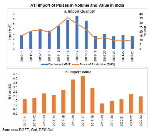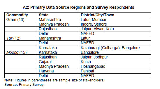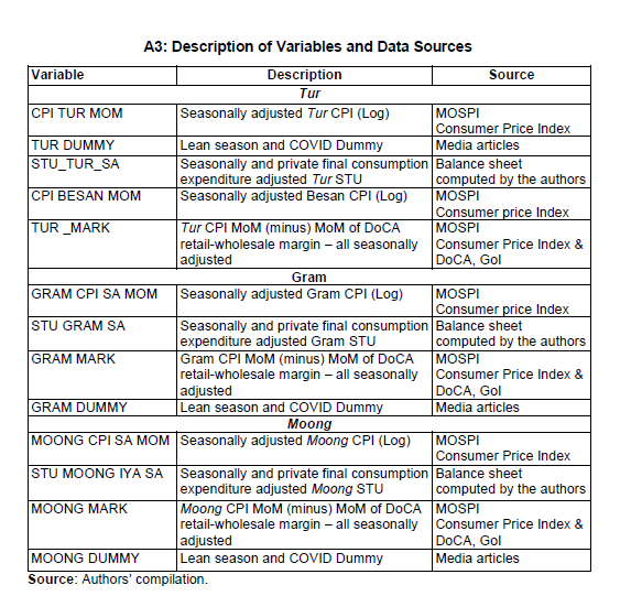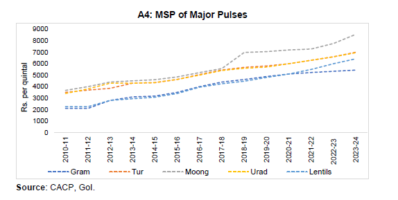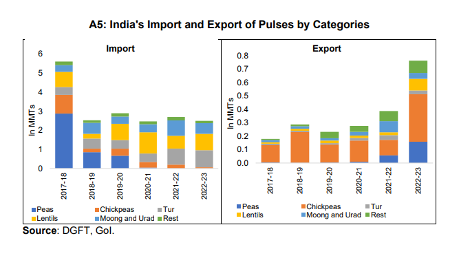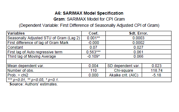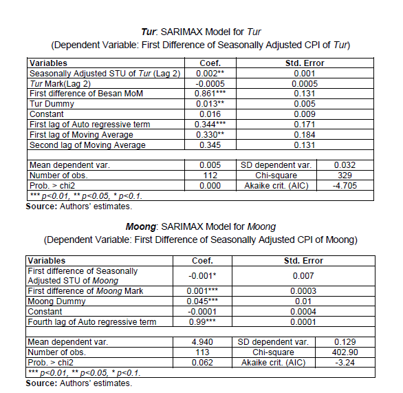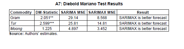

Annexure

¹ This study is part of a joint research project on “Understanding Price Dynamics of Major Agricultural Commodities and Identifying Ways to Improve Value-chains” by the Reserve Bank of India (RBI) and the Indian Council for Research on International Economic Relations (ICRIER). Shyma Jose, Sanchit Gupta and Manish Kumar Prasad are researchers, Sandip Das is a former Senior Consultant and Dr. Ashok Gulati is the Distinguished Professor at the ICRIER. Asish Thomas George and D. Suganthi are Director and Manager, respectively in the Monetary Policy Department (MPD) and Thangzason Sonna is Director in the Department of Economic and Policy Research (DEPR), RBI. The authors thank G. V. Nadhanael, internal discussant from RBI and an anonymous external reviewer for their valuable comments and suggestions. The views expressed in this paper are those of the authors and do not represent the views of the institutions to which they belong.

2 Food and beverages group has a weight of 54.18 per cent in CPI-Rural and 36.29 per cent in CPI- Urban.

3 The Reserve Bank of India Act, 1934, was amended in May 2016, paving the way for a FIT framework for monetary policy, stating the primary objective of monetary policy as maintaining price stability while keeping in mind the objective of growth. In August 2016, the Government of India notified a medium- term inflation target of 4 per cent, with a tolerance band of +/- 2 per cent. Subsequently, in March 2021, the Government retained the inflation target of 4 per cent, with a tolerance band of +/- 2 per cent for the period April 1, 2021 to March 31, 2026.

4 Among the bottom 30 per cent of the population based on monthly per capita expenditure classes, food accounts for 60.3 per cent and 55.0 per cent of the total expenditure in rural and urban households, respectively, in 2011-12 (MOSPI and WFP, 2019). The National Sample Survey Office (NSSO), Ministry of Statistics and Programme Implementation, Government of India has released the summary results of Household Consumption Expenditure Survey (HCES) conducted during August 2022 to July 2023 relating to estimated Monthly Per Capita Consumption Expenditure (MPCE) in the form of a factsheet in February 2024 and the detailed report in June 2024.

5 These include Russia’s export restriction on wheat, Indonesia’s ban on palm oil exports (which was lifted later on), Argentina’s ban on beef export as well as the ban on a variety of grain products by Turkey, Kyrgyzstan and Kazakhstan.

6In 2022, the global production of pulses was about 96 Million Metric Tonnes (MMTs) and India contributed about 27.7 MMTs (about 26 per cent) (FAOSTAT 2022).

7NSSO released the factsheet for the Household Consumption Expenditure Survey (HCES) 2022-23 in February 2024 and the detailed report in June 2024.

8Most kharif pulses like urad and moong have shallow root zones, while tur has slightly deeper rooting, which makes it tough enough to withstand droughts (SANDRP, 2015).

⁹ https://nipgr.ac.in/NGCPCG/Breedings%20of%20Chickpea.html

10 The SAE for 2023-24 does not include summer crop for Moong. In TE 2022-23, share of moong in total pulses production was 12.6 per cent.

¹¹ The proportion of the amount that a farmer receives from retail price paid by the consumer for a food item reflects the efficiency of an agriculture supply chain.

12Competitive storage model was first introduced by Gustafson (1958) and developed further in the work of Samuelson (1971) and Deaton and Laroque (1992).

¹³ The item-wise monthly Consumer Price Index (CPI) data is unavailable for March, April, and May 2020. Therefore, to address this gap, the study has imputed commodity-wise CPI values using the available CPI sub-group data for those months.

¹⁴ The SAE for 2023-24 does not include summer crop for moong production.

¹⁵ The buffer stock is created through the PSF and the PSS being implemented by the GoI’s Ministry of Agriculture and Farmers’ Welfare.

¹⁶ On February 12, 2022, the Ministry of Finance notified to remove the 10 per cent AIDC on imports of lentils with immediate effect, which further got extended till March 2024.

¹⁷ As the data on yellow pea imports is unavailable before the year 2019, we have taken the total pea imports as its proxy as more than 80 per cent of the total pea imports are that of yellow peas.

¹⁸ The gram and tur mark-ups are computed based on Latur mandi in Maharashtra, a key growing point for consumer prices at the urban centres like Mumbai, Indore, Hyderabad and Delhi, while moong mark- up is computed based on Jaipur, Rajasthan, a key growing point for consumer prices at the urban centres like Mumbai and Delhi.

¹⁹ An attempt was made to accommodate minor variations in specific pulses in terms of harvesting and arrivals time which differ across different agro-climatic regions, estimates of losses and wastages according to various studies and reports, conversion ratios for pulses, and consumption pattern across region and months. However, no significant improvement was observed as regards the robustness of the relationship between respective STUs and CPIs.

²⁰ NSO has released factsheet for household consumption expenditure survey for 2022-23 in February 2024, however, the commodity wise details including quantities are not yet available.