 IST,
IST,
RBI WPS (DEPR) : 7/2012: Measures of Nominal and Real Effective Lending Rates of Banks in India
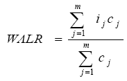
| RBI Working Paper Series No. 07 Abstract 1 In a bank-dominated financial sector, lending rates play an important role in the transmission of monetary policy. Yet, it is difficult to observe both nominal and real interest rates in the real time. Even ex post computation of effective nominal and real rates is challenging as banks' effective lending rates differ significantly from their reference rate such as the prime rate earlier or now the base rate. We present measures of nominal and real effective lending rates under the assumption of adaptive inflation expectations for banks for the period 1992-2010. The analysis suggests that real lending rates have declined in the recent years from their peak levels in the early 2000s and there is statistically significant negative relationship between real output growth and real interest rate. JEL Classification: E43, E23, E50 Key Words: Interest Rates, Monetary Policy, Interest Rate Channel Measures of Nominal and Real Effective Lending Rates of Banks in India I. Introduction Interest rate channel is considered as an important channel of monetary policy transmission. Therefore, the level and structure of interest rates are critical determinants of the economic efficiency with which resources are allocated in an economy (Mohanty, 2009). Among the various market interest rates, bank lending rates in the credit market play a pivotal role. The policy rate change by a central bank coupled with the underlying liquidity conditions first transmit to the short-term rates in the financial market and then to the bank lending rates which, in turn, is expected to transmit to the real economy, viz., growth and inflation over time so as to achieve the desired monetary policy objectives. In a bank-dominated financial sector, lending rates play an important role in the transmission of monetary policy. Yet, it is difficult to observe both nominal and real interest rates in the real time. Even ex post computation of effective nominal and real rates is challenging as banks' effective lending rates differ significantly from their reference rate such as the prime rate earlier or now the base rate. Against this backdrop, the objectives of this paper are three fold: First, to compute a time series on effective nominal bank lending rates. Second, to compute a time series of effective real lending rates. Third, to analyse the impact of changes in real lending rates on the real economy. This paper is organised as follows. Section II briefly traces the process of deregulation of bank lending rates in India. Section III develops a method of estimation of weighted average bank lending rate (WALR) from granular credit data based on the BSR system. Section IV gives a computation of real effective lending rates. Section V gives the linkage between aggregate output variables such as GDP with real lending rates. Section VI concludes. II. Deregulation of bank lending rates Till the late 1980s, the interest rate structure in the banking sector in India was largely administered in nature and was characterised by numerous rate prescriptions for different activities. Borrowers were charged significantly different rates for the same loan amount thereby distorting the structure of lending rates. Following the wide ranging financial sector reforms initiated in the 1990s, the interest rate structure in the banking sector has been progressively deregulated. Moreover, efforts have been made to rationalise the interest rate structure so as to ensure price discovery and transparency in loan pricing system. The process of rationalisation culminated in almost complete deregulation of lending rates by October 1994 except for small loans of credit limit up to `200,000. First, the credit limit size classes of scheduled commercial banks, on which administered rates were prescribed, were gradually compressed during 1990-93. Second, a system of prime lending rate (PLR), the rate charged for the prime borrowers of the bank, was introduced in October 1994. Since then for almost a decade till March 2003, the PLR system went through several modifications from a single PLR to multiple PLRs and tenor-linked PLRs and banks were given increasingly greater freedom in setting lending rates. The system of Benchmark Prime Lending Rate (BPLR) was introduced in 2003, which was expected to serve as a benchmark rate for banks’ pricing of their loan products so as to ensure that it truly reflected the actual cost. However, the BPLR system fell short of its original objective of bringing transparency to lending rates. Competition forced the pricing of a significant proportion of loans far out of alignment with BPLRs and in a non-transparent manner. There was also widespread public perception that the BPLR system had led to cross-subsidisation in terms of underpricing of credit for corporates and overpricing of loans to agriculture and small and medium enterprises. The Reserve Bank of India's (RBI) Annual Policy Statement 2009-10 (April 2009) noted that since the bulk of bank loans were lent at sub-BPLR rates, the system of BPLR evolved in such a manner that it had lost its relevance as a meaningful reference rate. The lack of transparency in the BPLR system also caused impediment to the effective transmission of monetary policy signals. Accordingly, the RBI set up a working group to examine the BPLR system (Chairman: Deepak Mohanty). On the basis of the recommendations of the Working Group and after taking into account the views of various stakeholders and discussions with banks, final guidelines on the base rate system were announced on April 9, 2010. With the introduction of the base rate system in July 2010, all categories of loans were to be priced only with reference to the base rate with a few exceptions. Since the base rate is stipulated as the minimum rate for all loans, the existing stipulation of BPLR as the ceiling rate for loans up to `200,000 was also withdrawn. A brief chronology of the progressive deregulation of lending rates is given in Annex I. III. Computation of effective weighted average nominal bank lending rates The nominal weighted average lending rate (WALR) for scheduled commercial banks (SCBs) is computed on the basis of granular data from the Basic Statistical Returns (BSR). BSR-1 return captures detailed data on outstanding bank credit as at end-March every year reported by banks in two parts, BSR-1A and BSR-1B (details in Annex II). BSR-1A captures data on credit outstanding and interest rate as at end-March for each loan account classified as Large Borrowal Account (LBA). In BSR-1B, credit data consolidated at branch level for Small Borrowal Accounts (SBA) are captured. From 1999, accounts with credit limit more than `200,000 are classified as LBA and those with credit limit up to `200,000 are classified as SBA2. The WALR is computed for the LBAs using BSR-1A data as follows:
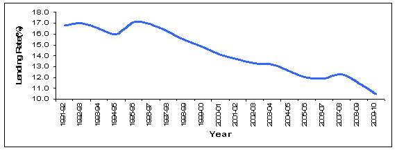
Where for loan account j, the interest rate charged is ij and the loan amount outstanding is cj as at end-March of a particular year; m is the number of accounts for which WALR is computed. The series of WALR for banks computed for LBAs3, both at aggregate level and at the sectoral level for the period 1992-2010 is given in Annex Table 1. The nominal WALR for the banking industry as a whole has shown a gradual decline (Chart 1). It has come down from a range of 16-17 per cent in most part of the 1990s to about 10.5 per cent by March 2010. The declining trend is clearly visible in the 2000s.
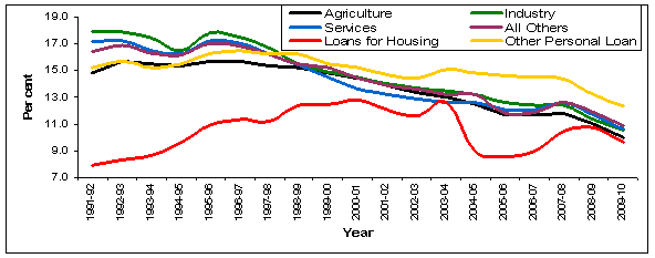
The declining trend has been broad-based across all sectors although it was somewhat muted in the category of other personal loans (Chart 2). The trend in interest rate on housing loan is an exception for certain reasons. In the 1990s, banks were not very active in the housing loan market as is seen from its low share in total bank loans till 2000. The bulk of the individual housing loans represented staff loans extended at concessional rates.
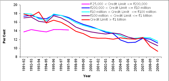
In the case of agriculture also, the nominal WALR declined to 10 per cent in 2010 which was hovering around 15 per cent in the 1990s. Similar decline was also visible in the case of industry and services. We also computed WALR for classification of loans according to credit limit (Annex Table 2). The trends in nominal WALR for different size classes of credit limit shows across the board decline in the lending rates (Chart 3).
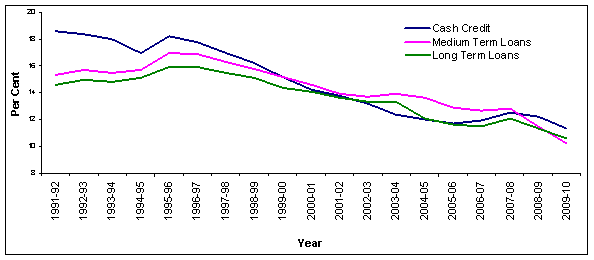
WALR has also been computed for various types of loans such as cash credit, medium term loans4 and long term loans 5 (Annex Table 3). Following the general trend, lending rates have come down in all the segments (Chart 4). While the shares of cash credit, overdraft and packing credit in the total credit declined over the period, the share of “medium and long term loans” has increased. Decline in the share of cash credit was prominent from 42.5 per cent in 1992 to 17.3 per cent by 2010. On the other hand, share of long term loans increased from 29 per cent in 1992 to 46 per cent in 2010. Even though WALR for all types of accounts has declined significantly, decline in cash credit, overdraft and demand loan was relatively higher at over 7 percentage points. In case of long term loans, the decline in WALR was about 4 percentage points. In other types of accounts, decline in WALR was around 5 percentage points.
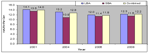
WALR for Small Borrowal Accounts (SBA) For small borrowal accounts (SBA), interest rate details are available periodically on survey basis6. The weighted average interest rate for the SBAs was worked out based on the size class-wise tabulations of the loan accounts data which was collected through the small borrowal accounts survey for the major sectors. For each sector, the amount outstanding against each occupation in the different interest rate range was used as the weight. The WALR presented in Annex Table 4 reveals declining trends similar to the interest rates for LBAs at aggregate as well as sectoral level. The combined WALR for all categories of loans (LBAs and SBAs) has been computed and shown in Annex Table 5 and Chart 5.
IV. Computation of real effective lending rate
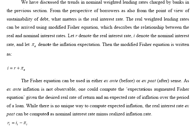
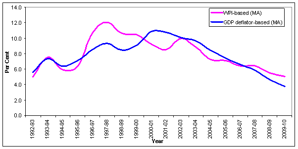
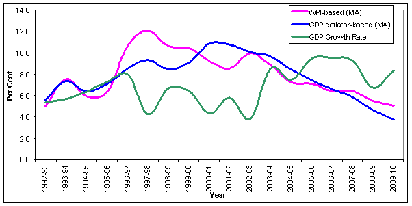
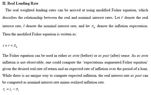
As investment decisions are made over a medium-term horizon, it is important to consider real lending rates in a medium-term perspective. Borrowers tend to view the nominal lending rate in terms of a desired real rate of return and expected inflation. Although several methods, including surveys, are employed to calculate expected inflation, it is difficult to assign expected values with a reasonable degree of precision given the uncertainty surrounding the future outcomes. This is more pertinent to developing economies like ours which are subject to structural economic factors and unanticipated supply shocks (Mohanty, 2010). Another useful way to address this issue is to derive expectations by smoothing the inflation series. This presupposes that expectations are adaptive, which is often the case in economies and markets with asymmetric information. Furthermore, given monetary policy credibility, the underlying inflation expectations are generally stable but for the deviations caused by short term volatility due to transitory factors. In our context, computation of real interest rate, even in an ex post sense, becomes challenging because of lack of a comprehensive measure of consumer price inflation. Hence, this paper considers two alternative ex post measures of real lending rates based on: (i) the wholesale price index (WPI), which is our headline measure of inflation; and (ii) the GDP deflator, the most comprehensive measure of inflation. If one assumes the inflation expectations to be adaptive then one could consider taking a larger time frame for economic agents’ memory than just pertaining to the immediate time interval. Following Mohanty (2010), a two-year moving average series of inflation rate to represent adaptive inflation expectations and for estimating ex post real lending rates have been used7. The annual series of real lending rates is given in Annex Table 6. It can be seen from the Chart 6 that the Real Lending Rate (RLR) based on both WPI and GDP deflator after peaking to double digits in early 2000s declined thereafter.
V. Real lending rates and economic growth Next we explore the relationship betweenreal output variables, viz., GDP growth and real lending rates. Technically, the real GDP growth is a measure of average real rate of return in the economy. Ideally, the real lending rates should not be too much out of alignment with the real GDP growth rate (Mohanty, 2010). The data for the period 1991-92 to 2009-10 show that real lending rates were higher than real GDP growth particularly during 1997-98 to 2002-03. This scenario has clearly changed since 2003-04 concurrent with the high growth phase of the Indian economy. The weighted average real lending rate has since remained below the real GDP growth rate (Chart 7).
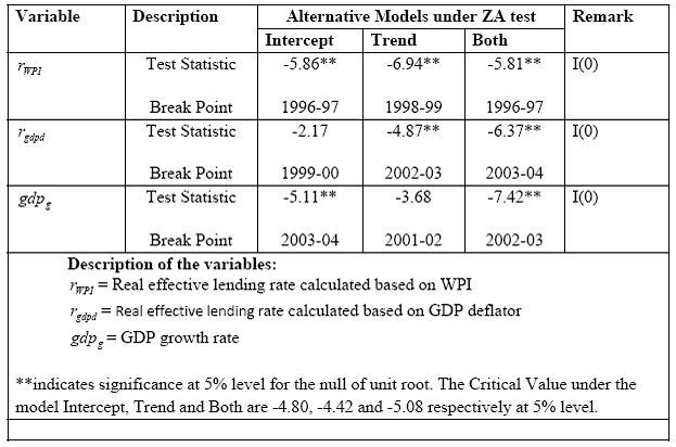
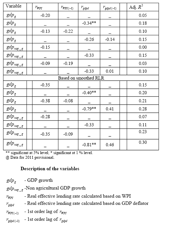
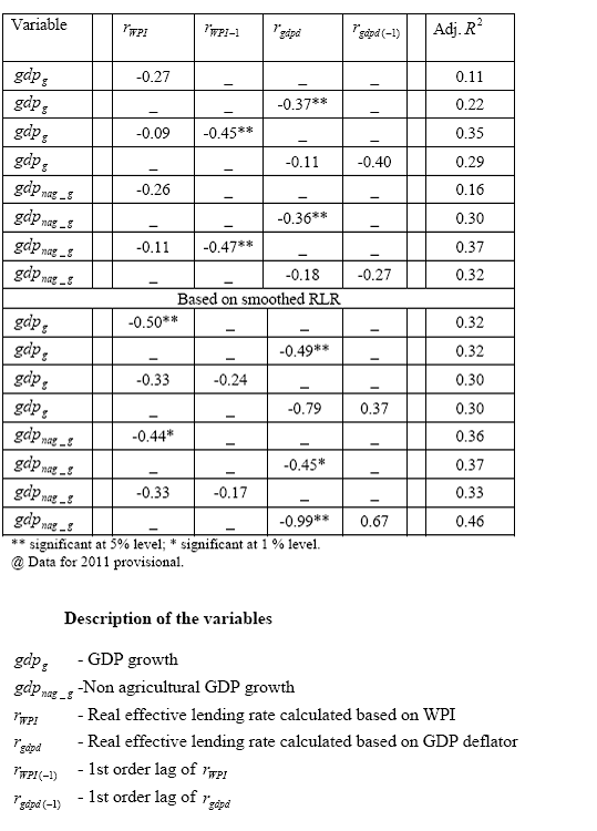
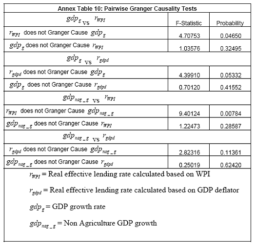
More formally, we test the relationship between output variables and RLR (based on WPI and GDP deflator) in a simple regression framework. We use both the annual RLR and also a smoothed series of two-year moving average RLR. We found a structural break in the RLR series in 1998, perhaps reflecting deepening of interest rate deregulation in late 1990s. Before proceeding with the regression, the variables were tested for stationarity based on Zivot-Andrews test (Methodology of the test is given in Annex III) allowing for one structural break. The RLR based on WPI and GDP deflator as well as the growth rate of GDP are found to be I(0) (Annex Table 7). Based on the outcome of stationarity tests, we have proceeded with the regression with growth rate of GDP (gdpg)/ non agricultural GDP (gdpnag_g) as the dependant variable and the RLR based on WPI / GDP deflator as explanatory variable. The relevant equations for the data period 1992-2010 are summarized in Annex Table 8. The hypothesis of inverse relationship between the output variables and RLR is validated by the sign of the coefficients. The significance of the coefficients and the variation explained (Adj. R2) improved in the case of non-Agricultural GDP and when smoothed RLR based on GDP deflator is used. The exercise is then repeated for the period 1997-2010, keeping in view the stage of deregulation and structural break (Annex Table 9). The relationship improves to some extent with RLR based on GDP deflator turning significant for GDP growth. Further, using the smoothed series, RLR based on both WPI and GDP deflator turns significant for GDP as well as Non-Agriculture GDP, indicating that with deregulation of lending rates, output has become more sensitive to real interest rate. Further, we also attempted causality analysis. Using Pair-wise Granger Causality test for full sample, it is found that real lending rate based on WPI (rWPI)Granger causes GDP growth (gdpg)and Non-agriculture GDP (gdp nag_g )(Annex Table 10). However, the results may be taken as broad indications only as the sample size is rather small. As interest rate deregulation progressed in the 1990s and the lending rate regime changed frequently, there was significant change in the loan pricing mechanism by banks. However, in order to assess the changes there is a need for a comprehensive measure of nominal effective lending rate for the commercial banks as a whole. We compute an annual time series on weighted average lending rates for bank credit in India for the period 1992-2010 based on the comprehensive BSR database. The WALR series so constructed makes available a larger dataset than used earlier. This is expected to bridge an important data gap for empirical assessment of the bank lending rate channel of monetary transmission, as hitherto such analysis had to rely upon BPLR data available for banks. WALR in nominal terms for the banking industry as a whole and across all sectors has shown a gradual decline. Further, the hypothesis of inverse relationship between output and real lending rate derived from nominal WALR based on WPI and GDP deflator is tested in a simple regression framework. The results were on the expected lines. Moreover, the strength of the relationship improved in the period 1997-2010 reflecting the effects of progressive deregulation of lending rates which enhanced the sensitivity of output to interest rate. @ The authors are Executive Director, Officer-in-Charge and Assistant Adviser, respectively, of the Department of Statistics and Information Management, Reserve Bank of India. 1 Views expressed in the paper are those of the authors and not of Reserve Bank of India. 2 The change in the share of loans of different sectors (Annex Table 1) in 1999 compared to 1998 was partly due to a change in classification of loan accounts. From 1999, the credit limit for loan accounts to be treated as LBA was increased from `25,000 to `200,000. As a result, a large number of small value agricultural loans were reclassified as SBA and were not captured in BSR-1A data used for computing WALR. 3 Till 1998, WALR is computed for loans with credit limit > `25,000 and from 1999 onwards, WALR is computed for loans with credit limit > `200,000. This has only a marginal and temporary impact on the share of agricultural loans and does not appear to have a significant impact on the trend in WALR. 4Loans and advances granted for a period of above 1 year and up to 3 years. 5 Loans and advances granted for a period of above 3 years 6 WALR for SBA was calculated for the years for which the survey of small borrowal accounts was conducted. Account level data for small borrowers are not available for rest of the period. 7Use of past actual inflation and its moving average as one of the proxy measures of ex ante adaptive inflation expectation is common in the literature (e.g. Taylor (1993); Bradford Delong (2002)). We consider two year as a relevant period prior to which the weights of past inflation could be small under assumption of adaptive inflation expectation. 8 A number of RRBs were amalgamated during the period. References Bradford Delong (2002): University of California, Berkeley, Lecture Notes in Macroeconomics, Chapter 12. Mohanty Deepak, (2010): "Perspectives on Lending Rates in India", speech delivered at the Bankers’ Club, Kolkata, June 11. Reserve Bank of India, (2009): Annual Policy Statement, April Reserve Bank of India, (2009): Report of the Working Group on Benchmark Prime Lending Rate (BPLR): Chairman Shri Deepak Mohanty, October Taylor, John B (1993): Discretion versus Policy Rules in Practice, Carnegie-Rochester Conference Series on Public Policy. Annex I: Evolution of Lending Rate Structure in India – A Chronology
Annex II: A brief history of BSR The Basic Statistical Return (BSR) system was introduced in 1972 to capture the micro level information on credit, deposits and investments of scheduled commercial banks (SCBs) which are otherwise not captured through regulatory returns. Currently there are seven returns (BSR-1 to BSR-7) under BSR system. As the objective of these returns has been to capture granular level information, most of these returns are collected at branch level. Among these returns, detailed bank credit information is captured under BSR 1 return. It is an annual return consisting of two parts (A & B) capturing outstanding bank credit as on end-March. To report data in BSR 1, the accounts are classified into either of the two groups called Large Borrowal Account (LBA) and Small Borrowal Account (SBA) based on their credit limit. Under Part A (BSR-1A), account level details for LBA (currently accounts with credit limit more than `200,000) are captured. Under Part B (BSR-1B), branch level credit data are collected for SBA (currently accounts with credit limit upto `200,000. A number of modifications were made in the BSR 1 system over time in January 1978, January 1984, January 1990, March 1996, March 2002 and March 2008. Some of the important changes introduced in BSR 1 are as follows:
At present, BSR 1A return captures for each LBA the following main items of data:
In BSR-1B return, the following data aggregated over the individual loan accounts are collected at branch level for SBA in two buckets viz. upto `25,000 and above `25,000 but up to `200,000.
Detailed loan account-wise information of SBA is collected based on a sample survey known as the Survey of Small Borrowal Accounts, which has been conducted at periodic intervals of 3-4 years. Data on interest rates with reference date as on 31st March is collected in the survey since 2001 and is available for the years 2001, 2004, 2006 and 2008. There has been a steady growth in the branch net of the Indian banking system (Table below). While the total number of bank branches of SCBs (including RRBs) went up almost six times between 1972 and 2010, number of loan accounts increased at a much faster rate during the same period. This large database maintained by the Reserve Bank is a rich source of granular historical data on bank lending in India, which forms the basis for computation of effective weighted average lending rate in this paper.
Annex Table 1:- Trends in WALR for all loans and for main sectors for SCBs – End-March
Annex Table 2: WALR according to Credit Limit as on 31st March for SCBs
Annex Table 3: WALR according to Type of Accounts as on 31st March for SCBs
Annex Table 4: WALR trends for Small Borrowal Accounts – All loans and main sectors
Annex Table 5: WALR based on all accounts
Annex Table 6: Real Lending Rate (RLR) based on WALR
Annex Table 7: Unit Root test with one Structural Break (Zivot-Andrews test)
Annex Table 8: Regression Analysis Results for the Period 1992-2011@
Annex Table 9: Regression Analysis Results for the Period 1997-2011@
I. WALR based on BSR 1 The nominal weighted average effective lending rate (WALR) for scheduled commercial banks (SCBs) is computed on the basis of granular data from the Basic Statistical Returns (BSR). In the BSR, interest rate applicable as at end-March is captured under Part A for each loan account. The WALR is computed as follows.
Where for loan account j, the interest rate charged is ij and the loan amount outstanding is cj as at end-March of a particular year; the number of accounts for which WALR is computed is m.
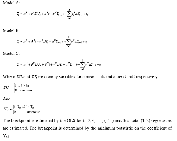
III. Methodology for Zivot-Andrews test The Zivot-Andrews test is a sequential Dickey-Fuller unit root test that test for a unit root against the alternative of trend stationary process with a shift in mean (Model A), a shift in slope (Model B) and a shift both in slope and intercept (Model C). The different models used are:
| |||||||||||||||||||||||||||||||||||||||||||||||||||||||||||||||||||||||||||||||||||||||||||||||||||||||||||||||||||||||||||||||||||||||||||||||||||||||||||||||||||||||||||||||||||||||||||||||||||||||||||||||||||||||||||||||||||||||||||||||||||||||||||||||||||||||||||||||||||||||||||||||||||||||||||||||||||||||||||||||||||||||||||||||||||||||||||||||||||||||||||||||||||||||||||||||||||||||||||||||||||||||||||||||||||||||||||||||||||||||||||||||||||||||||||||||||||||||||||||||||||||||||||||||||||||||||||||||||||||||||||||||||||||||||||||||||||||||||||||||||||||||||||||||||||||||||||||||||||||||||||||||||||||||||||||||||||||||||||||||||||||||||||||||||||||||||||||||||||||||||||||||||||||||||||||||||||||||||||||||||||||||||||||||||||||||||||||||||||||||||||||||||||||||||||||||||||||||||||||||||||||||||||||||||||||||||||||||||||||||||||||||||||||||||||||||||||||||||||||||||||||||||||||||||||||||||||||||||||||||||||||||||||||||||||||||||||||||||||||||||||||||||||||||||||||||||||||||||||||||
പേജ് അവസാനം അപ്ഡേറ്റ് ചെയ്തത്:


