 IST,
IST,
Chapter VI : Resilience of Indian Banking Sector
The resilience of the commercial banks in respect of credit risk, interest rate risk and liquidity risk were studied through stress testing by imparting extreme but plausible shocks. For the credit risk stress test a sensitivity analysis of capital adequacy ratios has been done by imparting shocks to the NPA levels. The interest rate risk has been studied through the Duration of Equity (DoE) method. The liquidity stress tests assess the ability of a bank to withstand unexpected liquidity drain without taking recourse to any outside liquidity support. The credit risk of the commercial banks has also been tested through a macro stress test model which links measures of credit risk to the macroeconomic variables. 6.1 Stress testing on the banking sector is undertaken on a continuous basis in the Reserve Bank to assess the resilience of the financial system to exceptional but plausible stress events. The stress testing undertaken normally uses single factor sensitivity analysis1 . In addition, a stress testing model which assesses the impact of macroeconomic variables on the financial soundness indicators of banks has also been attempted. In formulating the quantum of shocks, judicious criteria on selected indicators based on the experience of the Indian financial system are applied. The methodologies used in these stress tests are described in Annex-1. 6.2 The stress tests currently being conducted by the Reserve Bank on regular basis cover the following risks:
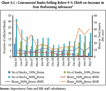
6.3 A macro stress testing model which assesses the impact of macro economic variables like GDP growth rate, interest rates, inflation and exports on the asset quality of banks and their capital adequacy ratio has also been presented. Credit Risk 6.4 The resilience of scheduled commercial banks to credit risk was tested by stressing the credit portfolio of banks with increases of 100 per cent, 200 per cent and 300 per cent in NPA levels as compared to the levels as at end-September 2010. At the aggregate level, a significant degree of resilience was observed and system CRAR remained in excess of regulatory requirements even under the most stressed scenario (i.e. an assumed increase in NPAs by 300 per cent). At the individual level, little deterioration in the CRAR of banks was observed when NPAs were assumed to increase by 100 per cent though the CRAR of several banks fell below regulatory requirements in case of assumed increases in NPAs by 200 per cent and 300 per cent. In the extreme case of an assumed rise in the level of NPAs by 300 per cent, the CRAR of about 20 banks accounting for a share of around 40 per cent of the total assets of the banking sector would fall below the regulatory requirement of 9 per cent CRAR (Chart 6.1). The credit risk stress tests, therefore, do not indicate any significant cause for concern except under extremely stressed scenarios.
Interest Rate Risk 6.5 Duration of Equity (DoE)3 of commercial banks shows an increasing trend in the recent quarters, pointing towards greater interest rate risk being assumed by banks (Table 6.1). This is also reflected at the level of individual banks with the number of banks with DoE between 10 years and 20 years having increased under the two assumed stress scenarios4 as compared to the position in December 2009, which was assessed in the last FSR (Charts 6.2 and 6.3). The increased interest rate risk assumed by the bank warrant careful monitoring.
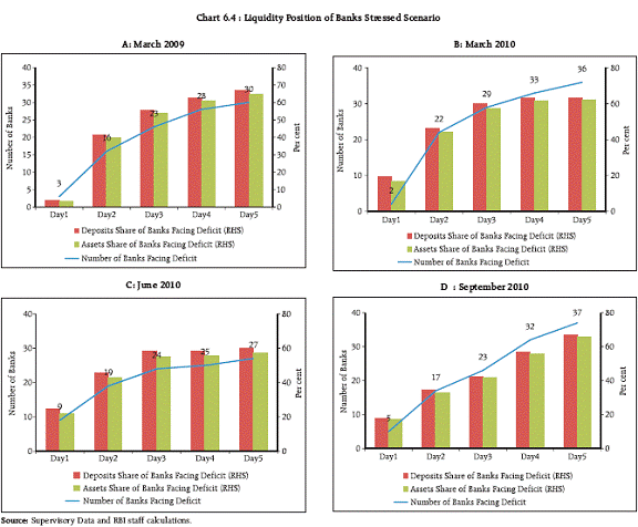
Liquidity Risk Commercial Banks 6.6 The liquidity stress tests assess the ability of a bank to withstand unexpected deposit withdrawal without recourse to any outside liquidity support. The scenarios have been developed based on stringent assumptions and assume unexpected deposit withdrawals in different proportions (depending on the type of deposits5 ). The tests assess the adequacy of liquid assets available to fund these withdrawals. The deposit run is assumed to continue for five days. 6.7 The stress tests showed that some banks did not have adequate liquid assets to meet the withdrawals on the first day itself. The number of such banks was higher in September 2010 as compared to March 2009 and March 2010 though there was some improvement as compared to June 2010. However, the total number of banks unable to withstand the stress scenario was higher in September 2010 compared to all the previous periods (Charts 6.4 A to D) indicating a slight worsening of the position under the liquidity stress tests relative to the previous assessment.
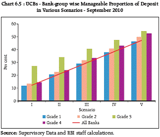
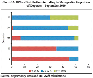
Urban Co-operative Banks 6.8 Stress tests on liquidity risk were conducted on the Scheduled Urban Co-operative Banks (UCBs) using their asset portfolio as at end-September 2010. Liquid assets forms 35.6 per cent of total assets and more than 88 per cent of total investments of the scheduled UCBs are in the form of SLR investments. 6.9 The stress tests for liquidity risk for the proportion of deposits, the withdrawal of which can be managed by the banks without any external assistance (i.e. through sale of their own investments) have been conducted for five assumed scenarios. At the aggregate level (aggregated for similar grade), the manageable proportion of deposits by the scheduled UCBs sector under various scenarios ranges from 12 per cent under scenario I (no liquidation of investments) for Grade 1 banks to 54 per cent for Grade 3 banks under scenario V (with 100 per cent liquidation of investments) (Chart 6.5 and Chart 6.6).
6.10 The results show that the liquidity position of scheduled UCBs is comfortable. The stress tests for manageable proportion of deposits in an event of a distress run on deposits (on account of sudden loss of confidence of investors) reflected that the scheduled UCBs have comfortable liquid portfolio to manage the stressed run on deposits. In a normal course of business (without sale of investments), the scheduled UCBs can overall manage a run of 12.2 per cent of total deposits without any external help. 6.11 In the worst scenario, which may force banks to liquidate all their investments, collectively they can manage a run of up to 47.2 per cent of deposits. Bankwise, except seven banks, all other banks can manage a run of more than 40 per cent of deposits. Macro-stress tests 6.12 Macroeconomic stress tests are increasingly considered as the basic, indispensible tool for any systemic efforts to reduce the likelihood and impact crisis events. Stress testing is basically a – ‘what if thinking’ – conducted in a structured manner (Box 6.1). 6.13 As an enhancement in the stress testing methodology, a preliminary beginning to model based approach for the macro-stress test has been made. The equations have been estimated which directly link macroeconomic variables to measures of bank performance. The ratio of non-performing advances (NPAs), defined as ratio of gross non-performing advances to total advances, has been chosen as the dependent variable from the list of financial soundness indicators. The macroeconomic variables have been classified into five groups (a) Growth indicators (b) Price stability indicators (c) Interest rates indicators (d) Financial Markets indicators (e) External sector indicators. In order to identify the significant risk factors from each group, bivariate regressions are estimated using a single macroeconomic risk factor with varying lags. The result of bivariate regressions gives a list of relevant variables from each group which could be considered for inclusion in the multivariate model. The scenarios are created using ‘shocked/ stressed’ variables by changing values of the independent variables. Macro stress-testing refers to a range of techniques used to assess the vulnerability of a financial system to “exceptional but plausible” macroeconomic shocks. Macro stress testing has been an important component of the Financial Sector Assessment Programs (FSAPs) launched by the IMF and the World Bank in the late 1990s and has become an integral part of the financial stability toolbox of policymakers. Macro stresstesting has received considerable attention in the last few years. Central banks and international organisations have taken the lead in this area of research, given their particular concern for financial stability issues. The two main methodological approaches to macro stresstesting are:
The foundation of macro-stress testing is built on the following steps: a. First step includes selection of the set of relevant financial institutions. A number of aspects need to be evaluated in this context. Should the analysis be restricted to specific section of the financial system or should it include all the sectors, for example, banks, non-banks, insurance companies, pension funds, etc.? Should the analysis be based on only the large banking institutions relevant for systemic stability? How to deal with financial conglomerates? Furthermore, the relevant portfolio for macro stress-testing depends partly on the nature of the risks to be analysed and partly on availability of accurate and granular data. b. Once the scope of the analysis covering a set of institutions and asset classes is identified, measuring risk exposure is the next task. Measurement of risk exposures is particularly challenging given the fact that portfolios are continuously evolving in response to specific investment and hedging strategies and in response to macroeconomic developments/shocks. c. Next is the determination of some key elements in the design of a stress scenario which includes the type of risks to analyse (market, credit, interest rate, liquidity and other risks); single or multiple risk factors to be shocked; parameter(s) to shock (prices, volatilities, correlations); size of the shock and time horizon. The analysis of a wider range of risk factors enhances the predictive power of the stress-test but imposes increased computational burdens. Similarly, simulating a comprehensive scenario including multiple shocks allows more realistic predictions than focusing on ad-hoc sensitivities of single parameters. d. The most important issue is the design of stress scenarios. One of the key decisions is how to calibrate the size of the shocks. Setting the size of the shock too low or too high might make the exercise unrealistic. In general, shocks can be calibrated to the largest past movement in the relevant risk variables over a certain horizon (or be based on historical variance). Alternatively, the estimated joint empirical distribution of past deviations from trend of the relevant risk variables can be used for simulating the stress scenario. Ideally, structural macro-econometric models should be employed to fully characterise the interacting shocks affecting key real economic indicators or asset prices that define the scenario of interest. Otherwise, the reduced-form reaction functions could also be used for scenario generation. References: 1. Cihak, M. (2007). Introduction to Applied Stress Testing. IMF Working Paper WP/07/59. 2. Foglia, A. (2009). Stress Testing Credit Risk: A survey of Authorities’ Approaches. International Journal of Central Banking, vol.6, no. 2. 3. Marco, Sorge (2004). Stress-testing financial systems: an overview of current methodologies. BIS Working Papers No 165. 4. Martin Melecky & Anca Maria Podpier (2010). Macroprudential Stress-Testing Practices of Central Banks in Central and South Eastern Europe. The World Bank. Policy Research Working Paper 5434. 5. Philippines: Financial System Stability Assessment Update (2010). IMF Country Report No. 10/90. April 2010. 6.14 Credit risk, represented by the ratio of NPA, is modeled by the logistic functional form in order to better capture tail risk and expressed as where the variable y can be interpreted as an index representing the state of the economy, which is associated with an improvement/deterioration in the credit quality of bank portfolios. The logit transformation6 is then assumed to be a function of exogenous macroeconomic factors (X) and a surprise factor represented by an error term, i.e.: Identification of significant risk factors 6.15 Initially, the non-performing advances ratios are regressed against various macroeconomic variables. The coefficients of these regressions provide an estimate of the sensitivity of bank borrowers to the relevant macroeconomic risk factors. where k represents the most significant lag. 6.16 The series consists of quarterly data from 1999 to 2010. The original data series have been transformed for getting stationary time series. The price variables, interest rate variables and exchange rate variables have been used in levels; the export and trade variables have been taken as ratio to GDP and the growth variables have been taken as annual percentage changes. 6.17 From the bivariate equations with large R2, the variables which have significant coefficients and having expected signs are selected for the multivariate equation. The variables chosen for bivariate regressions are given in Table 6.2.
Multivariate regression model: Estimates 6.18 Using the identified variables, a multivariate regression model is constructed, where the coefficients are significant, have expected signs and the residuals are stable. The model is described in Table 6.3. 6.19 The above model suggests that non-performing advances ratio is strongly auto-correlated. Further, NPA ratio rises with decline in agricultural or industrial GDP growth rates and vice-versa. The impact of agriculture is faster with 1 quarter lag, while the impact of industry is felt after 3 quarters. Moreover, the NPA ratio is positively related to short term nominal interest rate with 1 quarter lag. Finally, the NPA ratio rises with fall in export-to-GDP ratio with a lag of 2 quarters. The adjusted R2 is 0.98. 6.20 The Breusch-Godfrey LM test for autocorrelation in residuals shows no serial correlation in residuals. The White (heteroskedasticity robust standard errors) as well as Newey-West (for presence of both heteroskedasticity and autocorrelation) estimators for this specification are not very different and the test statistics for statistical significance of coefficients are generally unchanged. The regression results have been obtained using Newey-West variance estimator, to control for possible autocorrelation or heteroskedasticity in the presence of lagged dependent variables among the regressors. Stability diagnostics through examination of recursive residuals shows that the parameters of the model are stable across various sub-samples of the data. The stress scenarios 6.21 The calibrated model is used to forecast NPAs under the baseline as well as stress scenarios. The stress test risk horizon is for two years. Accordingly, the baseline and stress scenarios have been constructed (Table 6.4 and Table 6.5).
6.22 The forecast values of the ratio of the nonperforming advances under baseline and stress scenarios are given by the model (Chart 6.7).
6.23 The forecast values of the ratio of the nonperforming advances, derived from the model, have been translated into capital ratios under each scenario (Chart 6.8). The translation is based on a “balance sheet approach”, by which capital in the balance sheet is affected via the provisions and net profits. In order to estimate the new capital ratio under each scenario, the provisions coverage ratios were kept at the current level. Further, the credit growth, risk-weighted assets growth and profit growth have been assumed to be 20, 12 and 10 per cent, respectively. The forecasted increase in NPAs was distributed across sub-standard, doubtful and loss categories in the same proportion as prevailing in the existing stock of NPAs.
6.24 The results show that, amongst the list of macroeconomic variables in the aforesaid macro stress testing model, the impact of export shock on the gross NPAs ratio is the highest. However, the results under different scenarios, suggest that the macro-economic shocks would not substantially threaten the Indian banking sector. 6.25 As indicated above, the model described here encompassed the first steps towards putting in place an extensive macro stress testing framework to assess the build up of systemic risks in the system. In the coming periods, this methodology will continue to be developed so that it can become part of a growing number of tools that can be used to evaluate the soundness of individual banks and that of the financial system as a whole. Concluding Remarks 6.26 Stress tests of the credit risk exposure of banks reveal a reasonably comfortable position and resilience of banks to withstand unexpected deterioration in credit quality. However, some deterioration in the capital position of banks is seen in the assumed scenarios of doubling or tripling of the current NPA levels. The increasing trend in the Duration of Equity of commercial banks suggests more interest rate risk and therefore requires active monitoring. The liquidity stress test results show that some banks face liquidity constraints under the stringent stress scenarios both for commercial banks as well as UCBs. The liquid assets positions needs to be assessed and improved to meet any adverse economic condition. 6.27 The macro-stress test for credit risk exposures focuses on interdependence of credit risk and the state of the economy, as measured by macroeconomic variables. The results show that Indian banking sector is at a reasonably comfortable position and resilient to withstand unexpected deterioration in credit quality. The impact of shocks on macroeconomic variables constructed under various stress scenarios is found to be muted. However, risks to domestic macroeconomic variables arising from any further deterioration in the global economic conditions need to be monitored. Annex 1: Stress Testing Methodologies As a part of regular surveillance approach, stress tests were conducted covering the following risks:
The resilience of the commercial banks in response to the above shocks were studied from the above three perspectives. The analysis covered all scheduled commercial banks. The methodology adopted for the stress tests is in line with the stress tests conducted for the first FSR. These stress tests are single factor sensitivity analysis and do not take into account the inter-linkages of macroeconomic variables with the financial soundness indicators. Credit Risk To ascertain the resilience of banks, the credit portfolio was shocked by increasing NPA levels, for the entire portfolio, along with a simultaneous increase in provisioning requirements. The estimated provisioning requirements so derived were first adjusted from the annualised profit of the banks and the residual provisioning requirements, if any, were deduced from banks’ capital. The analysis was carried out both at the aggregate level as well as at the individual bank level, based on quarterly supervisory data from March 2007 through September 2010. The scenario assumed increase in the existing stock of NPAs by 100, 200 and 300 per cent and enhanced provisioning requirements of 1 per cent, 25 per cent and 100 per cent for standard, sub-standard and doubtful/loss advances, respectively. The assumed increase in NPAs was distributed across sub-standard, doubtful and loss categories in the same proportion as prevailing in the existing stock of NPAs. The additional provisioning requirement was applied to the altered composition of the credit portfolio. Interest Rate Risk The duration of equity (DoE) or the net-worth duration approach in stress tests could help in calculating the erosion in capital due to unit increase in interest rates. The analysis takes into account the interest rate sensitive items in balance sheet of the banks’ portfolio and also the banks’ exposure to interest rate sensitive off balance sheet items. Subject to certain limitations, DoE captures the interest rate risk and helps in moving towards the assessment of risk based capital. The higher the duration of equity, more is the interest rate risk and accordingly greater the requirement of capital.
Under this approach, the duration of equity of a bank’s portfolio is computed under two scenarios: the savings deposits are assumed to be withdrawn in the first time band viz. 1 to 28 days (scenario I); the savings deposits are assumed to be withdrawn in 3 to 6 months time band (scenario II). The time band-wise rate sensitive liabilities have been accordingly adjusted under the two scenarios. Liquidity Risk Scheduled Commercial Banks The aim of liquidity stress tests is to assess the ability of a bank to withstand unexpected liquidity drain without taking recourse to any outside liquidity support. The scenarios developed are based on very stringent assumptions, which are extreme. The analysis is done as at end-March 2009 through end-September 2010. The scenario depicts different proportions (depending on the type of deposits) of unexpected deposit withdrawals on account of sudden loss of depositors’ confidence and assesses the adequacy of liquid assets available to fund them. The deposit run is assumed to continue for five days.
Urban Co-operative Banks Stress test on liquidity risk were conducted on the Scheduled Urban Co-operative Banks (UCBs) using their asset portfolio as at end-September 2010. It is assumed that banks’ liquid assets such as Cash in hand, balances with banks, money at call / short notice and investments (SLR as well as non-SLR) are used for getting liquidity in times of stress before resorting to any external help. It is assumed that all the investments can be sold out at 10 per cent haircut during the period of deposit run. Other assets of UCBs such as, loans and advances, overdue interest receivable, premises, furniture, fixtures, bills purchased and discounted are treated as illiquid assets. The proportion of deposits run which can be managed by the UCBs without any external help (might be by the sale of investments) has been used for testing the resilience. For the purpose of stress test analysis on liquidity, five scenarios are considered wherein percentage of total investment portfolio of UCBs is considered which can be liquidated in times of stress. Scenario I describes sale of investments on account of (a) normal course of business without any stress, or (b) the extreme (though rare in practice) situations where banks have made all their investments in illiquid/ non-marketable securities, or (c) there is no market for banks’ investments on account of complete loss of confidence. In the most extreme stress of deposit run, the banks may need to liquidate their all the investments (i.e. 100 per cent) with assumed haircut, which is described as Scenario V. Other Scenarios include 25 per cent (Scenario II), 50 per cent (Scenario III) and 75 per cent (Scenario IV) liquidations of total investments with assumed haircut. The proportion of liquidation depends on extant of run on deposits to be managed. Macro stress test - Credit Risk To ascertain the resilience of banks, the credit risk was modeled as functions of macroeconomic variables. The analysis was carried out on ratio of non-performing advances to total advances at the aggregate level for the commercial banking system as a whole. With the help of the developed model the NPA ratio was forecasted for next few quarters. This included both baseline and stressed scenarios. On the forecasted values of NPAs, the capital adequacy ratios were derived keeping the existing loan loss provisions intact. 1 The stress tests undertaken are based on inputs taken from the Handbook on Financial Sector Assessment, published by the International Monetary Fund and the World Bank in September 2005. Drawing on this framework, the methodology was calibrated to suit domestic realities, taking on board the state of development of the financial system and the maturity of financial institutions and markets. This is the approach which was also used by the Committee for Financial Sector Assessment. 2 CRAR has been calculated under Basel I in order to obtain a sufficiently long time series of historical data. All Scheduled Commercial Banks (except RRBs and LABs) have moved to Basel II framework with effect from March 2009. 3 The Duration of Equity calculates the erosion in accounting capital due to a unit increase in interest rates. Higher the duration of equity, more is the interest rate risk. A DoE of 20 years implies that an interest rate shock of 500 basis points will be required to wipe out capital. 4 Savings deposits are assumed to be withdrawn in 1 to 28 days under scenario I while they are assumed to be withdrawn in 3 to 6 months under scenario II. The time band-wise rate sensitive liabilities have been accordingly adjusted. Scenario I implies a lower duration of liabilities and is the more stringent scenario of the two. 5 These are described in Annex I. 6 The logit transformation helps to map the original variable, which was bounded by 0 and 1, into a real line, which could be used in an ordinary linear regression equation. The logistic functional form is also convenient in that y is given by the logit transformation: |
|||||||||||||||||||||||||||||||||||||||||||||||||||||||||||||||||||||||||||||||||||||||||||||||||||||||||||||||||||||||||||||||||||||||||||||||||||||||||||||||||||||||||||||||||||
പേജ് അവസാനം അപ്ഡേറ്റ് ചെയ്തത്:


