8.1 The foregoing chapters covered a wide canvas of macroeconomic relationships underlying the growth process in India with a view to exploring the current slowdown, the scope for monetary and fiscal policy action, external levers of growth and the contribution of financial intermediation to the growth process in terms of allocative efficiency. Each chapter attempted to construct a bridge between the theory and the operational realities embodied in the functioning of the economy, both national and cross-country. In doing so, each chapter maintained its own identity in terms of approach, methodology, presentation and inference; however, a common thread runs through them all: a quest for the revitalisation of growth in the Indian economy. Accordingly, it is possible to summarise the findings of the Report into one unifying framework of accounting of the Indian economy.

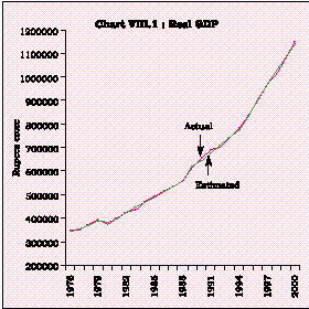
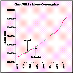
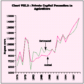
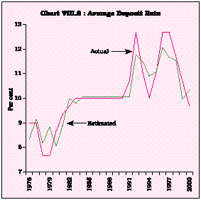
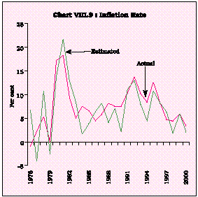
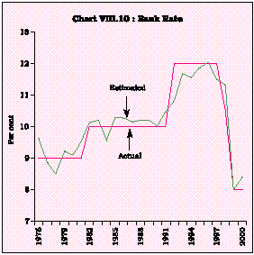
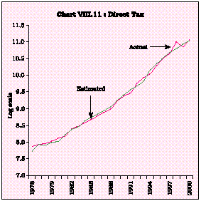
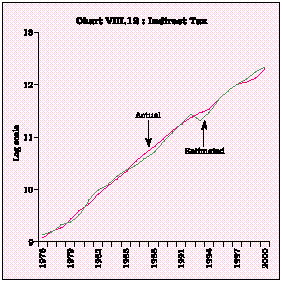
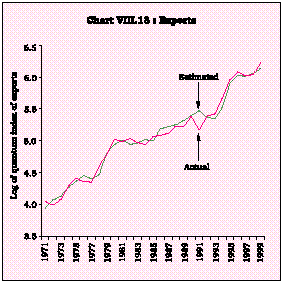
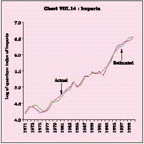
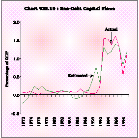
8.2 This chapter, therefore, attempts to present the estimated characteristics of sectoral behaviour, inter-linkages and the underlying dynamics of the overall economy in the form of a structural macroeconomic model. The model is small in the interest of facilitating a wider understanding as well as computational feasibility. It consists of 18 behaviorial equations and 23 identities representing the principal structural relationships identified in the preceding chapters. There are 26 exogenous variables including pre-determined variables in the model. It needs to be mentioned that the various other estimation exercises conducted in the earlier chapters are employed either as sub-models recursively feeding into the main model or as information variables enabling off-model consistency-check calibrations, although they may not be explicitly set out in this chapter. Moreover, certain parameters estimated in the preceding chapters may undergo some alteration when re-estimated in an integrated framework in this chapter, though the objective is not to deviate from the underlying theoretical postulates. The design of this chapter is as follows: Section I sets out the algebra underlying the construction of the model and its sectoral components accompanied by a commentary of the a priori expectations given by economic theory and the methodological issues confronted in actual estimation. Section II evaluates the model results in terms of the statistical criteria of robustness, and graphical depiction of the 'goodness of fit' of estimated equations. Section III simulates various possible scenarios obtained by delivering 'shocks' to key instruments with a view to deriving the implications for the strength and sustainability of the growth response.

I. THE MODEL

8.3 The model has the following distinguishing features: (i) recognising that aggregate demand shocks are temporary while aggregate supply shocks are persistent, the model is constructed with specific counter-cyclical properties so as to qualify as a policy model for evaluating stabilisation policies; (ii) it is flexible and capable of incorporating the impact of future changes in technology by suitably altering the parameters of the production function which enters the model in an off-model setting; (iii) it is built around the multiplier-accelerator principle which sets a law of motion for the macroeconomic variables; (iv) the model belongs in the modern tradition of ‘consensus models’ in which money does not explicitly find a place; competitive financial market conditions are assumed under which monetary and financial quantities clear through prices, i.e., interest rates and the role of money is taken by a monetary policy reaction function specified in an endogenous setting; and (v) it is forward-looking and can accommodate future revisions in inflation threshold/targets, which are determined off-model.

Real Sector Block

8.4 A macroeconomic model focusing on growth confronts the unavoidable problem of over-identification of the key parameter, i.e., GDP or Y. To resolve the problem, the analytical approach of Chapter III is adopted, i.e., the growth process is conceived as a combination of cyclical and structural influences, with the former predominantly determined by forces operating on aggregate demand and the latter reflecting conditions of aggregate supply. The behaviour

of aggregate supply ^(Ys⁾ can be estimated in the form of a simple production function of the Cobb-Douglas type in which output is largely determined by factor accumulation - fixed capital (K) and labour (L)- and factor productivity:

Ys = A Ka Lb

( 1)

where a + b = 1 only under conditions of constant returns to scale, and 1< a + b < 1 under conditions of increasing returns and decreasing returns, respectively. a and b are technical parameters representing the marginal product of capital and labour, respectively. In India, as in other developing economies, constant returns to scale may not be the appropriate assumption and, therefore, the generalised production function is employed where there are no restrictions on the parameters a and b. The parameters of the production function, which is estimated outside the model, are fixed and employed essentially to set the long run trajectory of aggregate supply. In equilibrium, aggregate supply must necessarily match aggregate demand, in a post facto sense; however, aggregate demand is an ex ante phenomenon in the sense that consumption and investment decisions by economic agents are planned, and the process by which aggregate demand and aggregate supply adjust represents the underlying dynamics of growth. Since planned aggregate demand may deviate from aggregate supply before the attainment of equilibrium in the post facto sense, it is necessary to specify the behaviour of aggregate demand in the model. The basic economy wide identity serves as the specification i.e.,

Yd=C+I+G+(X - M)

(2)

where Y_d is the aggregate demand, C represents consumption by the private sector, I investment by all agents in the economy, G government consumption, X exports of goods and services and M represents imports of goods and services.

8.5 As mentioned earlier, aggregate demand and aggregate supply can diverge in an ex ante sense. This divergence is the ‘structural output gap’ which provides a summary measure of cyclical changes in demand and thereby, of future inflationary expectations. The aggregate demand represents the behaviour of the four segments of the economy; i.e., households and businesses comprising the private sector, the government, and the external sector. The behaviour of each of the four major economic agents is modelled separately. The private sector - households and private business - affects overall demand by changing both C and I. Private consumption (real) is postulated to be a function of last year's income to capture the lags between income and spending, the real deposit interest rate (r_drt) and real government consumption (G) to capture crowding-out/crowding-in effects:

C = a + b1 Y(-1) + b2 rdrt + b3 G

(3)

8.6 Investment behaviour of the private sector could be studied in a disaggregated framework. First, total investment (real) can be broken down into its public and private components:

I = Ipv +Ip

(4)

where I _pv and I _p are private and public investment, respectively;

Secondly, private investment can be disaggregated under agriculture ^(I pv,ag^), manufacturing

(I_pv,mnf), services (I_pv,srv ) and others (I_pv,others), i.e.,

Ipv = Ipv,ag + Ipv,mnf + Ipv,srv + Ipv,others

(5)

8.7 In the third stage, the investment equations are modelled in the context of the accelerator principle. Investment responds to changes in income [DY(-1)] and also to the induced changes provoked by stabilisation policy (i.e., change in the real interest rate brought about by altering the nominal interest rate, given inflation expectations) and public expenditure which takes the form of infrastructural and producer services or I_p,srv (approximation for fiscal policy). Inclusion of the interest rate (r) as a determinant of investment assumes importance in view of the present stance of monetary policy that emphasises 'revival of investment demand through provision of adquate liquidity' and the scope for softening the interest rate stance if the evolving situation so warrants even while continuing with the stable interest rate environment (Monetary and Credit Policy, Reserve Bank of India, October 2001). The significance attached to the evolving situation in the decision regarding the interest rate also explains that the interest rate reaction function can be endogenised, even though depending on the weightage of judgement based policy action, the reliability of estimated coefficients could vary over time. Investment in agriculture is presumed to be impervious to interest rate changes given its preferential treatment in the policy framework.

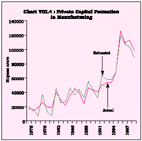
Ipv,ag

= c+ d1

D Y(-1) + d2 Ip, srv

(6)

Ipv,mnf	= e+ f1	D Y(-1) + f2r + f3 Ip, srv	(7)
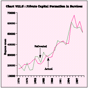
Ipv,srv	= g+ h1	DY(-1) + h2r + h3 Ip, srv	(8)

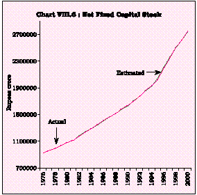
In the standard literature, capital stock would adjust in response to investment (adjusted for depreciation). In India, while consistent time series data on 'net fixed capital stock' for the economy as a whole are available, information on investment (i.e., gross capital formation) are available on a gross basis, warranting specific adjustments which cannot be presented in the form of an identity to link the capital stock accumulation process with investment. Gross capital formation represents a combination of fixed capital, working capital and depreciation. Thus, only a part of the gross capital formation could explain the capital stock adjustment process. Accordingly, the increment in the net fixed capital stock is modelled separately as,

DK =h4+ h5I

(9)

The above specification would also help in examining the supply response of output to changes in investment.

Monetary Block

8.8 The response of consumption and investment behaviour to change in real interest rates offers the scope for the operation of monetary policy in order to stabilise the real sector. The real interest rate has two components, i.e., the nominal interest rate (R_lrt, represented by the SBI advance rate) and inflation expectations (modelled in Chapter V):

r = Rlrt – p (-1)

10

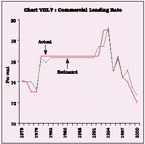
8.9 The nominal lending rate is specified asa function of the Bank Rate (R_brt) to establish the link between the policy rate and the lending rate:

Rlrt = l + m Rbrt

(11a)

Unlike investment in different sectors which get influenced by the lending rate (equations (6), (7) and (8)), consumption behaviour (in other words, saving behaviour) could respond to change in deposit rates (equation(3)). Assuming that the Bank rate is used as the key policy rate for anchoring the structure of interest rates in India, the deposit rate could be specified as

Rdrt = l1 + m1 Rbrt

(11b)

A positive and statistically significant m1 could validate the relationship between the bank rate and deposit rates as has been presumed while specifying the equation (11b).

8.10 A critical consideration guiding the conduct of monetary policy is the anchoring of inflation expectations. Actual inflation (p) can be expressed as a combination of the estimated inflation gap (p_gap) and the threshold inflation (p^T) which is estimated in Chapter V. In other words,

pgap = p - pT

(12)

8.11 The behaviour of the inflation (proxied by change in the inflation rate in the model (Dp)) is specified to respond to the observed behaviour of the output-gap (Y_gap- the difference between aggregate demand (Y_d) and aggregate supply (Y_s)) summarily representing the conditions of aggregate demand, as well as supply shocks to inflation originating from the foodgrain sector (measured by foodgrains prices-Dp _food).

Dp = j + k1 Ygap(Ly ) + k2 Dp food+k3Dp(Lp)

(13)

where L^y and L^p denote appropriate lags.

8.12 Equations 10 to 13 are specified in a manner which allows aggregate demand to respond to changes in the real lending rate. Furthermore, the monetary policy reaction function is also specified to examine the response of the Bank Rate to the behaviour of the output gap and the inflation gap. In Indian conditions, fiscal policy, in particular, the financing of the fiscal deficit has an important bearing in shaping the stance and setting of monetary policy. Accordingly, the fiscal deficit (fd) can be explicitly introduced into the monetary policy reaction function as follows:

Rbrt= n0 + n1Ygap(Lp ) + n2pgap+ n3fd

(14)

Fiscal Block

8.13 The conduct of fiscal policy in India is marked by the absence of a financing constraint. In order to capture this country-specific feature, public expenditure (G) is assumed as exogenous.

This is strategic since it enables testing of the possibilities of 'pump-priming' as well as alternative combinations of government expenditure which are decided outside the model. Non-tax revenues (NTR), mainly comprising profit transfers from the monetary authority and other public sector entities, user charges, etc., are also exogenous to the model.

8.14 Tax receipts (TR) comprise direct tax (DT) and indirect tax (IT) collections, i.e.,

TR = DT + IT

(15)

8.15 Both direct and indirect tax revenues are expected to be determined by aggregate income (Y) and price level (P) as a proxy for inflation tax, the latter is important for fiscal policy under a tight revenue constraint:

DT = p + q1 Y + q2 P		(16)
IT = r + s1 Y + s2 P		(17)

The price level is linked to the inflation equation (13) by

P = P(-1) (1+ p)

(18)

Given the exogenous public expenditure, interest payment (IP) and estimated tax revenues, the fiscal gap (FD) is represented as

FD = G + IP + Others - TR - NTR

(19)

and as a proportion to nominal GDP (representing the conventional presentation of the fiscal deficit in India),

fd = FD / Yn

(20)

Nominal income Yn (i.e., GDP at current market price) is obtained by reflating real income (Y-GDP at factor cost at constant prices) estimated in (2) by the GDP deflator (DFL)

Yn = (Y * DFL) + net indirect taxes

(21)

and the GDP deflator is specified in a linear relationship with the wholesale price level (P), i.e.,

DFL = u + vP

(22)

Similar deflators for different components of aggregate demand have also been estimated to provide the link between respective nominal and real variables.

External Sector Block

8.16 Net exports of goods and services are conventionally regarded as an injection of external demand supplementing aggregate domestic demand. In India, the typical situation is that, given the supply constraints, some part of domestic demand is satisfied externally, i.e., through imports. For countries with limited degree of external openness and continued reliance on sustainable current account targets, foreign capital inflows can meet the financing of net import demand and help in achieving other macro-economic objectives such as reserve adequacy.

8.17 Merchandise exports (quantum index of exports or xg) are postulated to be determined by world demand conditions (represented by changes in world GDP or Yw) and export prices in dollar terms as prevailing in India (PXD) and in the rest of the world (PXW)(to explain the relative profitability of selling in the domestic versus the world market).

xg = w0 + w1Yw w2PXD + w3PXW

(23)

8.18 Import demand, represented by quantum index of imports (m_g) is expected to be determined by domestic real GDP(Y), unit value index of imports(P_MD) in rupees in relation to domestic price-P (to explain the relative attractiveness of domestic substitutes versus imports), and debt service ratio (DSR) which embodies the foreign exchange constraint to imports.

mg = x0 + x1Y - x2PMD + x3P – x4 DSR

(24)

8.19 Assuming that prices of exports (P_XD) and imports are determined in the(P_MD) international markets and net services are exogenous, i.e., outside the model, nominal values of exports, imports and the current account balance are obtained through the following transformations:

Xg= (xg) * (PXD)

(25)

Mg = (mg)* (PMD)

(26)

(X-M) = (Xg-Mg) + net services

(27)

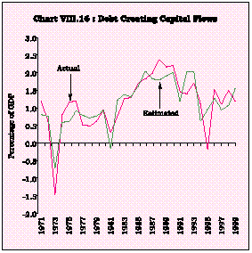
8.20 Having specified the external resource balance at (27), net capital flows can also be modelled as a mirror of the external resource balance in the current account with an adjustment for changes in reserves and other transactions which are not explicitly modelled but can explain the difference between actual capital flows and (X-M) such as, change in reserves, net transfers, net income, and errors and omissions. The indirect representation of the external resource balance through capital flows draws from the analysis presented in Chapter V and the capital flow equations are entirely off-model in nature. The net capital flows (NCF) can be disaggregated into net debt creating flows (DCF) and net non-debt creating flows (NDCF) as follows:

NCF = DCF + NDCF

(28)

8.21 Non-debt capital flows are expected to be influenced by the behaviour of debt service ratio-DSR (higher debt service ratio may encourage forced liberalisation of policies towards non-debt), degree of openness-OPN (reflecting both the needs for foreign capital as well as the capacity to service external liabilities), change in foreign exchange reserves-DFX (indicator of confidence) and depreciation of the domestic currency-DEPR (which could reduce the return in rupees when converted into US dollars). Debt creating flows, in turn, are expected to be determined by the debt service ratio-DSR (reflecting the need for additional capital to service the debt), import intensity of GDP-MGDP (another indicator of need for foreign capital) and non-debt capital flows-NDCF (as a policy of prioritising capital flows would imply that debt flows may only be encouraged when non-debt flows appear inadequate).

NDCF = z0 + z1 DSR +z2OPN + z3 fd + z4 DFX

-z5 DEPR(-1)

(29)

DCF = z6+z7DSR+z8MGDP(-1) +z9NDCF(-1)

(30)

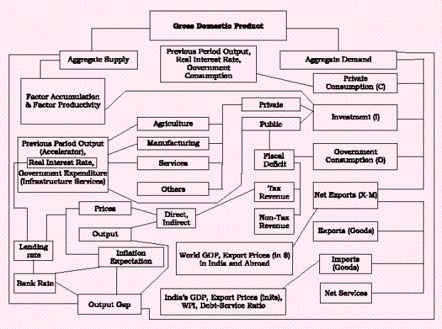
8.22 The dynamics of the model can be represented in terms of a flowchart (Box VIII.1). Annual data covering the period 1970-71 to 1999-2000 have been used for examining these dynamics. Seventeen dummy variables were also used in different equations, to approximate the effects of outliers.

II. THE RESULTS

8.23 The empirical results are reasonably robust and satisfy the usual statistical properties of significance and goodness of fit. The order condition is satisfied with respect to individual equations and there is no problem of identification. All equations are satisfactory in terms of a priori signs.

8.24 Estimates of the relative contribution of capital and labour to the aggregate supply of output as per the specification set out in equation (1) show that while capital stock exhibits unit elasticity with output, the elasticity in respect of labour turns out to be about 0.22. In view of the evidence supporting increasing returns to scale and the strong impact of capital accumulation on growth, raising the investment rate appears to be the critical force for strengthening the supply response and increasing the long-run capacity output.

8.25 As regards the relative importance of aggregate demand, private consumption demand has significant relationship with permanent income (as proxied by lagged income) and government expenditure. The real interest rate shows a negative impact on private consumption as expected, indicating the positive response of savings to real return. The partial elasticity of private consumption to government consumption indicates contemporaneous complementarity of private consumption with public consumption spending, although the inter-temporal effects would be consistent with crowding out effect.

8.26 Different components of private sector investment behaviour respond differently to changes in major determinants. Private investment in agriculture seems to be influenced by lagged aggregate output only modestly, indicating the weak operation of the accelerator. Public sector expenditure on infrastructure related services - including power - has a somewhat moderate influence on private investment in agriculture. Private investment in manufacturing sector strongly responds to public investment on infrastructure and previous period output - the latter indicating the smooth operation of the accelerator. Private investment in manufacturing shows a statistically significant negative relationship with the real interest rate. Thus, reducing the real interest rate can play a catalytic role in stimulating private investment. Financial intermediation (FIMD) has positive effect on private investment.

8.27 Pubic sector investment expenditure on services strongly influences private sector investment in the service sector with a relatively strong accelerator, which is, however, less effective than in case of private investment in the manufacturing sector. The real interest rate also exhibits a statistically significant and negative relationship, as in the case of investment in the manufacturing sector.

BOX VIII.1:STRUCTURE OF THE MACROECONOMIC MODEL

8.28 Direct tax revenue, as expected, is strongly influenced by both real GDP and the price level. The income effect, however, clearly dominates the price effect. In respect of indirect tax revenue, the opposite result is obtained as the price effect outweighs the income effect. This clearly signifies the effect of strong pass-through of increase in indirect tax rates to the final prices.

8.29 Changes in inflation rate seem to have responded strongly to the anticipated output gap. Changes in food prices also show the expected positive relationship with headline inflation. The negative relationship with previous period inflation suggests evidence of some correction in agents' expectations as also the effect of anti-inflationary policy stance. In the monetary policy reaction function, the Bank Rate seems to have responded more to output gap than the inflation gap, indicating a pro-active response of monetary policy in terms of stabilising the real economy. The Bank Rate setting incorporates the impact of the fiscal stance on financial market conditions. The lending rate exhibits significant relationship with Bank Rate over time, signifying the determining influence of monetary policy on the structure of interest rates in India.

8.30 Estimated income elasticities of exports and imports indicate that net external demand could be an important source for stimulating output growth in India. As per Krugman's (1989) 45-degree hypothesis, the income elasticities of demand for a country's export and imports are systematically related with a country's long-term GDP growth. Fast growing countries generally exhibit a high income elasticity for their export and a modest/low income elasticity for their imports. Estimated income elasticities for India (over the period 1970-2000) show that the income elasticity of exports (2.03) is almost twice that of the income elasticity of imports (1.03), implying that export-led growth can ensure a faster rate of GDP growth for India than other countries having an export to import elasticity ratio of less than two. The relatively higher sensitivity of exports to fluctuations in world GDP relative to the sensitivity of imports to fluctuations in domestic output indicates that during a global recession, higher trade deficit could weaken the export-led growth process, unless the terms-of-trade and export supply conditions improve simultaneously.

8.31 Both export and import demand exhibit price sensitivity, with exports increasing when international export prices in US dollar (P_XW) increase in relation to the prices for Indian exports in US dollar (P_XD). Similarly, imports seem to increase when prices of domestically available goods (as reflected in P) increase in relation to the prices of importables (P_MD). While the former shows the relevance of competitive pricing to augment export growth, the latter testifies the role of relative cost advantage of import substitutes in containing the growth of imports. For enhancing both the competitive pricing of exports and domestic production of cost effective import substitutes in a policy environment that is free from any export or import bias, productivity enhancing real investment would be critical. Productivity induced output growth would reinforce the growth enhancing effects of an export-led growth strategy.

8.32 Given the role of capital flows in the growth process, an assessment of the determinants of capital flows with an emphasis on the pull factors suggest that both openness and fiscal deficit turn out to be statistically important in influencing non-debt capital flows. The fiscal deficit seems to discourage non-debt inflows while greater trade openness potentially attracts larger inflows. Higher debt service (representing greater need for foreign capital) and annual increment to the country's foreign exchange reserves (which enhances the confidence about repatriability) seem to be associated with higher inflows whereas rupee depreciation seems to discourage inflows. Debt creating flows are primarily driven by the need for financing and, therefore, exhibit statistically significant co-movement with import intensity of GDP, debt service ratio and fiscal deficit.

Estimated Equations

(1) Production Function (Log Linear form)

LnY =

2.49 + 1.02*LnK + 0.22*LnL - 0.065*D80s

	(-13.3)	(16.6)	(1.8)	(8.7)
Adjusted R2= 0.99 DW = 2.2
Ln denotes for natural logarithm.

(3) Private Consumption

C = 72493 + 0.55 Y(-1) - 597 rdrt + 1.07 G

(20.86)

(13.27)

(-2.49)

(3.51)

+ 13066 D80s + 18066 D97,99

(7.23)

(3.78)

Adjusted R2 = 0.99, DW = 2.50

(6) Private Agricultural Investment

Ipv,ag=3837 + 0.06 DY(-1) + 0.08 Ip,srv

(6.05)

(5.27)

(4.30)

+2896 AGDUM

(7.36)

Adjusted R2= 0.89, DW = 1.57.

(7) Private Manufacturing Investment

Ipv,mnf = -44952 + 0.52 D Y(-1) - 728r + 1.28 Ip,srv

(-2.86)

(2.37)

(-3.37)

(5.69)

+31571FIMD + 31832 D96 - 22908 D90

(1.72)

(2.77)

(-2.75)

Adjusted R2 = 0.87, DW = 1.57.

(8) Private Service Sector Investment

Ipv,srv = -25745 + 0.26D Y(-1) -463r + 0.78 Ip,srv

(-4.45)

(3.11)

(-3.05

(6.66)

+28421 FIMD

(3.82)

Adjusted R2 =0.88, DW = 1.98

9. Net Fixed Capital Stock

DK = -15106 + 0.56 I

(-1.6)

(10.3)

Adjusted R2 = 0.94, DW= 1.60

(11a) Commercial Lending Rate

Rlrt = -1.14 + 0.75 Rlrt (-1) + 0.52 Rbrt

(-1.80)

(12.93)

(5.05)

-4.30 D95 + 3.00 D76,97

(-7.20) (8.84)

Adjusted R2= 0.96, DW = 2.09, h = -0.28

(11-b) Average Deposit Rate (Rdrt)

Rdrt = 4.30+ 0.59 Rbrt + 0.95 D78,93,96 + 0.80 AR (1)

(2.82)

(4.13)

(3.69)

(6.28)

Adjusted R2= 0.88 DW = 1.65

(13) Inflation Rate

Dp= 0.57 Ygap + 0.39 Dpfood - 0.26 Dp (-2)

(1.93)

(3.57)

(-1.83)

-0.25 Dp (-4) + 5.00 D80 - 2.18 D96

(-1.88)

(1.67)

(-2.88)

Adjusted R2= 0.67, DW = 2.28

(14) Monetary Policy Reaction Function

Rbrt = 0.81 Rbrt (-1) + 0.06pgap (-1) + 0.18 Ygap(-1)

(14.17)

(2.90)

(1.92)

+ 0.06fd - 1.50 D98

(1.72)

(-3.51)

Adjusted R2= 0.88, DW = 2.12, h = - 0.27

(16) Direct Tax

LnDT = -14.68 + 1.58*LnY + 0.68*LnP + 0.17*DT77

(-6.5)

(7.8)

(5.9)

(8.3)

+ 0.21*DT9499

(3.3)

Adjusted R2= 0.99 DW = 2.0

(17) Indirect Tax

LnIT =-7.33 + 0.97 LnY + 1.30 LnP - 0.16 IT75

(-3.4)

(5.0)

(12.7)

(-4.7)

- 0.28 IT9399

(-5.5)

Adjusted R2= 0.99 DW = 1.5

(23) Export Demand

Lnxg = - 6.68 + 2.03 LnYW + 0.99 LnPXW

(-2.01)

(3.89)

(3.41)

-0.63*LnPXD+ 0.82*AR(1)

-(1.92)

(6.93)

Adjusted R2 = 0.98, DW= 1.84

(24) Import Demand

Lnmg=-9.15 + 1.02 LnY - 0.81 LnPMD

(-3.94)

(4.89)

(-8.02)

+ 1.29 LnP – 0.01 DSR

(6.49)

(-3.92)

Adjusted R2 = 0.99,DW =1.27

(29) Non-Debt Capital Flows

NDCF = -1.05 + 0.02 DSR + 0.12 OPN - 0.12 fd

(-4.25)

(1.82)

(7.78)

(-2.48)

+ 0.006 DFX -0.07 DEPR(-1)

(2.83)

(-2.19)

Adjusted R2 = 0.80, DW=0.85

(30) Debt-Creating Capital Flows

DCF = -1.11 + 0.02 DSR(-1) - 1.31 DUM

(-2.69)

(4.55)

(-4.77)

+ 0.21Yn(-1)) - 1.02 NDCF(-1)

(4.72)

(-4.26)

Adjusted R2 = 0.67 DW=2.23

III. SIMULATING THE MODEL FOR ATERNATIVE POLICY SCENARIOS

8.33 The model is operationally evaluated by simulating it using the Gauss-Seidel algorithm. The model's predictive power is attested by the simulation error statistics, e.g., Theil's 'U' statistics for some key endogenous variables (Table 8.1).

	Table 8.1 : In-Sample Prediction Error Statistics

	Behavioural Equations/Variables		Theil's U Statistics
	1		2
1.	Private Consumption		0.01
2.	Private Investment in Agriculture		0.01
3.	Private Investment in Manufacturing		0.10
4.	Private Investment in Services		0.01
5.	Capital Stock Accumulation		0.03
6.	Production Function		0.01
7.	Direct Taxes		0.02
8.	Indirect Taxes		0.03
9.	Exports		0.05
10.	Imports		0.03
11.	GDP Deflator		0.01
12.	Inflation Rate		0.07
13.	Lending Rate		0.19
14.	Deposit Rate		0.31
15.	Bank Rate		0.18
16.	Deflator(Government Investment)		0.01
17.	Deflator(Government Consumption)		0.02
18.	Deflator (Net Exports)		0.06

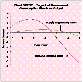
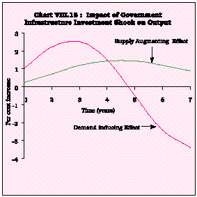
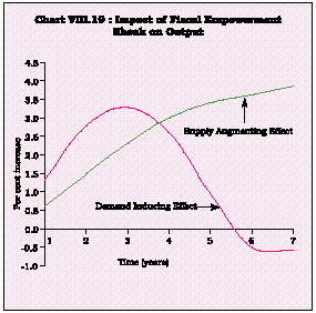
8.34 Given the performance of the model, five scenarios are generated to evaluate (i) the impact of fiscal stimulus through (a) a sustained increase in government consumption expenditure by 5 per cent; (b) a sustained increase in government investment expenditure in infrastructure services by 5 per cent; (c) a sustained enhancement in fiscal empowerment by reducing government consumption expenditure by 5 per cent accompanied by a matching increase in government investment expenditure in infrastructure; (ii) the impact of monetary stimulus through a one-time one percentage point reduction in the Bank Rate; (iii) the impact of external demand conditions through an increase in the world GDP by 1 per cent on a sustained basis. It needs to be recognised that each shock has a dual effect i.e., a demand inducing as well as a supply augmenting effect .

8.35 The shock to government consumption produces a demand induced expansion in output which is, however, short-lived, lasting in intensity up to 3 years before losing momentum. Output declines thereafter with the cumulative loss of output completely offsetting the initial gain from the shock. Simultaneously, the shock yields a marginal improvement in the supply response embodied in capacity output (Chart VIII.17).

8.36 The stimulus through government investment in infrastructure has a similar effect on aggregate demand as that of government consumption, but the impact on aggregate supply is pronounced and persistent (Chart VIII.18).

8.37 Switching the shock by reducing government consumption with an offsetting increase in government investment in infrastructure has a major impact on aggregate supply, i.e., capacity output which rises in a sustained manner over the full period of the shock. Demand effects are similar to those obtained earlier, although they do not completely offset the initial stimulus, as in the case of a pure government consumption shock (Chart VIII.19).

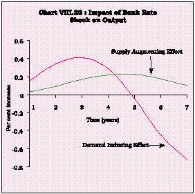
8.38 The monetary policy shock conveyed through a reduction in the Bank Rate generates a modest improvement in demand induced output which is transient and less powerful than the fiscal expansion. The impact on capacity output is lower than the impact of pure government consumption and pure government investment shocks (Chart VIII.20).

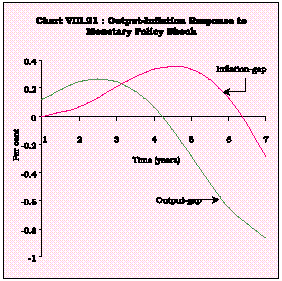
Keeping in view apparent inflation-growth tradeoff associated with any monetary policy shock the output-gap effect has been compared with the inflation-gap effect by giving a shock of one percentage point reduction in the bank rate (Chart-VIII.21). The positive output response dominate in the initial years, but over time the output response subsides while the inflation effect predominates and persists for a long period.

8.39 Finally, the external demand shock produces weak demand and supply effects, almost replicating the effects of the monetary policy shock. Thus, under the current conditions of sluggish demand, both external and internal, monetary policy and external demand have limited roles to play in the revitalisation of growth (Chart VIII.22).

IV. CONCLUDING OBSERVATIONS

8.40 The macroeconomic model presented in this chapter provides a synoptic view of an economy experiencing an adjustment of demand to the supply constraints. Aggregate demand is sensitive to interventions by stabilisation policies; however, these stimuli are short-lived, even episodic, and unable to retain potency in the absence of an upward shift in the aggregate supply curve. This requires releasing the sectoral bottlenecks inhibiting productive capacity expansion through both factor accumulation and increased productivity. In the context of the increasing returns to scale characterising the production process, this acquires importance as it can potentially be exploited to shift out the production possibility frontier so that even higher growth rates of the economy than recorded so far can become feasible.

8.41 The current deceleration in the economy has front-loaded fiscal policy, already under the stress of ongoing fiscal consolidation, with responsibilities for stabilising the economy. Yet, fiscal reform of the 1990s is being viewed as having eroded the efficacy of fiscal policy as a stabilisation instrument and this is being put to the stress by the current phase of activity. Public investment has become the 'soft target' of consolidation as in many other countries in similar proces of transformation. Public investment has, however, externalities which can be reaped by private investment, particularly in infrastructure. Faced with the conflict between the compulsions of downsizing and the objective of stimulating the revival of the economy, discretionary fiscal stabilisers seem to have been used in the form of an expansion in both government consumption and investment expenditure. The results obtained here indicate that the impact of a consumption stimulus is temporary, and can reverse to dampen aggregate demand over time. It needs to be recognised, however, that even while public investment has stimulating and complementary effects for private investment, the consequent expansion in the fiscal deficit can result in financial crowding out, raising the real interest rate via the nominal interest rate and this, in turn, can induce a downturn in aggregate demand. Accordingly, fiscal stimuli in support of revival of growth must rely on a compositional shift in fiscal expenditures in favour of public investment in infrastructure without an unbridled expansion of the fiscal deficit.

8.42 A stimulus to aggregate demand can also be applied through expansionary monetary policy through its influence on real interest rates. Output effects are positive in the short run, losing force as the inflation effect dominates over time. There are non-linearities in the growth-inflation relationship which need to be taken note of by monetary authorities. Identifying the threshold inflation is critical for the monetary policy reaction function. The current inflation rate in India has fallen below the threshold estimated for India. The threshold itself has a shifting perspective, responsive to underlying inflation conditions. The pursuit of controlling inflation below the threshold as an objective of monetary policy has adverse output consequences. In India, sacrifice ratio-the output costs of disinflation, can go up to 2 per cent of real GDP for every one percentage reduction in inflation.

8.43 Capital flows have begun to matter in the growth process. So far, the growth-inducing properties of external capital flows have remained unexploited due to lack of absorptive capacity. A 'pecking order' in inflows is clearly in existence in India but this hierarchy seems to be policy induced. Maintaining full debt servicing and adequate reserve levels are 'feel good' factors while fiscal deficit needs to be contained to encourage augmented inflows of non-debt capital.

8.44 The Report is exploratory and its findings formative, requiring the validation of time. Identification of factors underlying the current deceleration is an empirical quest. Quantification matters from the point of view of calibrating the policy response. Revitalising growth has assumed a global urgency; the scope for discretion in national efforts is getting bounded by the inertial dynamics of the slowdown. For India, a measure of insulation from global conditions provides some discretion to seek within for country-specific solutions. In this regard, the principal impediment emerges as the inadequate response of private investment to the change in the development strategy. Catalysing private investment could be the central focus of the second generation of reforms. This may require transformation in the policy framework, including a reconsideration of the public and private incentive structure to spur and modulate the flow of investment demand. Consumption levels are, however, protected including through public intervention. Here external flows have a role to play in smoothing consumption, and preventing the deceleration in the rate of domestic saving and investment. This, in turn, has implications for external viability. The key role of exports comes to the fore. The financial sector can contribute to the revival in a supply-leading role as well as by improving the overall productivity of the economy through allocative efficiency gains. The financial sector, comprising financial institutions and markets, may well nurture the first impulses heralding the upturn.

8.45 The urgency attached in this Report to the revitalisation of growth is enmeshed in a recognition of the basic impediments to sustained development - the high incidence of unemployment and the lack of tangible gains in poverty reduction. There is a growing consensus for an agenda of reforms which directly address these fundamental obstacles to progress. Creating an environment for investing in human and physical capital, labour market and industrial reforms, removal of pricing distortions, farm policy re-orientation, legal restructuring and fiscal empowerment by rebalancing fiscal instruments will help to address the gaps in employment generation and poverty alleviation. The translation of this agenda into action would be facilitated by a favourable macroeconomic environment as an initial condition.

---