 IST,
IST,


Inflation and Inflation Expectations: A Distributional Mapping
|
by R. K. Sinha ^ The article analyses statistical characteristics of the Consumer Price Index-Combined (CPI-C) based inflation and inflation expectations datasets and identifies suitable statistical distributions for these. The identification of appropriate distributions facilitates in establishing a one-to-one mapping of these distributions. The mapping provides a conversion/correspondence of a data point from one dataset to another. These models have the potential to forecast inflation and are also potentially useful to measure Inflation-at-Risk (IaR). Introduction The CPI-C based inflation data is published by the Ministry of Statistics and Programme Implementation (MoSPI) together with granular-level data. One type of granularity is by-product item at the all-India level. Another is according to the product group and sub-group level according to States/Union Territories (UTs) and Regions (Rural/Urban). The Reserve Bank conducts the Inflation Expectations Survey of Households (IESH), which provides expectations of the respondents (surveyed households) on inflation for the near term. Such surveys are known for biases internationally, and accordingly, the levels of inflation expectations often differ from the realised inflation. Nevertheless, they have proved to be very useful for tracking the directional changes. Several recent studies (Das et al., 2019; Shaw, 2019; Muduli et al., 2022) have attempted to assess the inherent biases in such surveys and removed them to establish a meaningful comparison between inflation and inflation expectations. In this article, we carry out a comparative study of the statistical characteristics of entire distribution of the datasets of actual inflation of MoSPI and inflation expectations 1 of the surveyed households rather than just modelling and mapping the central tendencies of the two datasets. It may please be noted that comparing and modelling aggregate inflation/inflation expectation numbers often lose inherent information in the dataset, as these are just the derived numbers. The article is divided into five sections. After the introductory section, the datasets of inflation and inflation expectations are described in the second and third sections, respectively. The fourth section connects the findings of these two sections through suitable mappings and suggests possible uses of it. The last section concludes the article. II. Statistical characteristics of CPI-C based Inflation Dataset The data on CPI-C based inflation (aggregate as well as granular level) is published by the MoSPI on a monthly frequency. Statistically, the mean of inflation of the aggregate and granular-level datasets of the same period should match closely, the standard deviation (SD) of granular data can be expected to be higher as compared to the SD of aggregate data, as aggregate data is a distribution of the mean of the granular data. The modal inflation of the aggregate data falls in the band of 5 per cent to 6 per cent, while it is in the band of 4 per cent to 5 per cent in the case of disaggregate data for the period January 2014 to June 2023. The greater variability in the granular data represents individual product level shocks, which can be favourable (bringing the aggregate level inflation towards target point) or adverse (moving away the aggregate level inflation from the target point). The lowest and highest inflation in the aggregate level data stand at 1.46 per cent (recorded in June 2017) and 8.60 per cent (recorded in January 2014), respectively during January 2014 to June 2023 (Chart 1). 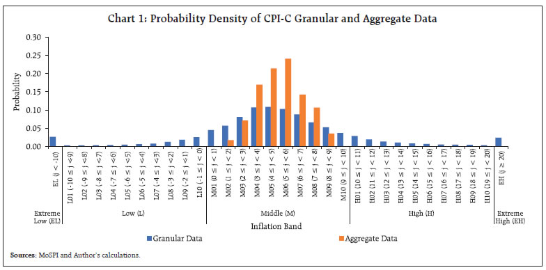 The distribution of inflation in the granular level has varied significantly across the months driven by the relative presence of extreme values. We attempt to analyse the statistical properties of the granular dataset 2 over the period January 2014 to June 2023. The disaggregated dataset of CPI-C may, initially, appear to have some characteristics of a normal (bell curve). 3 However, the dataset is found to be very leptokurtic i.e., having high peak than normal, with a kurtosis at 15.856. The distribution visually appears to be more-or-less symmetric, although has a mild positive skewness of 0.869. A best fit Normal distribution, viz., N (5.0430, 7.1185) is also plotted, demonstrating the nature of poor fitting with under-estimation at around central and extreme values, and compensating over-estimation in between (Chart 2). The underlying leptokurtic dataset has fatty tails with around 2.5 per cent of observations each in extreme parts, i.e., inflation lower than -10 per cent in the left tail and more than 20 per cent in the right tail, representing severe shocks (Chart 1). As the normal distribution fails to explain characteristics of the dataset, we explore and search for other suitable statistical distributions, which may potentially explain the nature of this dataset. It is observed that no single statistical distribution explains the dataset adequately. Two best-fit distributions were identified as Cauchy (μ = 4.7930 and σ = 2.4758) and Laplace (μ = 5.0430 and λ = 0.1987) though they also do not fit the dataset appropriately (Chart 2 and Table 1). 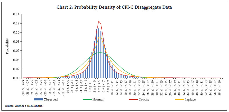 It may be mentioned that the granular level dataset is composed of various product/sub-product groups across the regions (Rural/Urban) and States/ UTs leading to wide heterogeneity. Fitting of sub-sets of datasets by product categories, having larger heterogeneity than regions and States/UTs, indicate more precise modelling for some of the products. Also, we observe larger variations in the descriptive statistics of these subsets. For example, inflation of ‘cloth and footwear’ appeared to be closest to a bell curve (normal); inflation of ‘housing’ hovered in a tight spread (narrow range) over time ( Annex - Chart A1 and Table A1). If a single distribution fails to fit the underlying dataset appropriately, various studies have explored and demonstrated the use of mixture distributions, having potential to capture the characteristics of the dataset more appropriately. These mixture distributions can be constructed with or without the identification of a threshold, a particular value of the random variable. The threshold approach partitions the dataset into two parts, and the parts are modelled separately using different statistical distributions. Several studies e.g., Cooray and Ananda (2005) and Scollnik (2007) used the Lognormal-Pareto model; Ciumara (2006) and Scollnik and Sun (2012) applied the Weibull-Pareto model; Nadarajah and Bakar (2014) suggested Lognormal-Burr model; to mix two distributions with a threshold. Other approaches suggest mixing of two statistical distributions across the entire distribution without any threshold, but that might have fixed or dynamic weights (mixing parameters). Frigessi et al. (2002) demonstrated a dynamic mixture model for the unsupervised tail estimation without estimating the threshold. The study used a Weibull-Pareto pair, which assigned a higher weight, starting from one, to Weibull at the left part of the distribution which is gradually reduced and tend to zero at the right tail of the distribution. All these studies demonstrated the same dataset viz., Danish fire loss data, a famous insurance dataset known for its heavy right tail. Unlike the above dataset, which has only one possible heavy tail loss, as values are bounded at zero, the underlying inflation dataset has two clear tails, which have varied significantly across the months. We split the data into two parts with inflation at 4 per cent, as the threshold. These two parts of the dataset are modelled separately. However, we transform the data before the modelling as detailed below: Let {xL} and {xR} are the data points of the initial granular dataset of inflation covering the distinct ranges (-∞ to 4 per cent) and [4 per cent to ∞), respectively. We define: 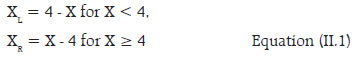 Both, XL and XR range from 0 to ∞ now. We now fit the data and identify that 3-parameter Burr and 3-parameter Dagum 4 are the two distributions, which could explain the characteristics of the data appropriately for both the parts. We use Burr distribution in our case, and rest of the analysis is centered around Burr. Burr distribution is a versatile distribution and has been found to be suitable for many insurance datasets. Sastry and Sinha (2010) used a 4-parameter Burr distribution to describe Danish fire loss data and found it to be competitive to several mixture distributions, as proposed by some of the studies for this dataset, as mentioned earlier in this section. The probability density function (pdf) of a 3-parameter Burr distribution is defined as: 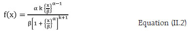 Where, k (>0) and α (>0) are the first and second shape parameters, respectively; β (>0) is the scale parameter. The distribution function (df) of a 3-parameter Burr distribution is defined as: 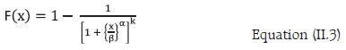 The descriptive statistics (DS) of each part of the distribution indicates resemblances of observed data and fitting by Burr (Table 2). The fitting by using mixture distribution indicates stark improvement over the initial approach of using single distribution. Now the derived variables (XL and XR) are transformed back to the original variable (X) and the modelled probability density functions are proportioned into their respective weights and stitched together. This way, the derived single pdf from the synthetic pair of Burr (2.2685, 1.1129, 5.6631) and Burr (2.7037, 1.2135, 7.9923) adds to unity with appropriate weights 5 and explains the data in a much better way (Chart 3). 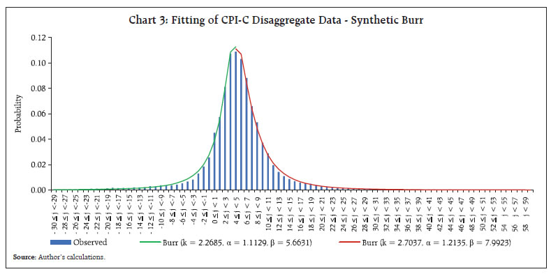 If a single distribution, whether derived on a standalone basis or through the mixing of distributions, fails to capture the characteristics of extreme tails adequately and precisely, its estimates of probabilities in the extreme tails are neither reliable nor usable, as it may be under or over-estimating these consistently. In such cases, the alternative solution is to model the extreme tails exclusively through the Extreme Value Theory (EVT) tools. In the current case, the synthetic Burr appears to fit well the entire curve including the tails (Chart 3). We examine the same statistically and explore if EVT tools would be a valuable addition in this context. The distribution of excesses over a high threshold, say u, in the right tail of inflation is defined as: 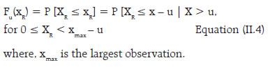 The distribution of excesses represents the probability that inflation (X) exceeds the threshold inflation u by at most an amount xR, where, xR = x-u, given the information that X exceeds the threshold u. In terms of the underlying function, the same is as below: 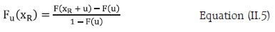 The functions, Fu(xR) and F(xR + u), are the conditional and unconditional distribution functions, respectively. The function F(xR + u) is equivalent to F(x), as x R = x - u. The F(u) is the cumulative probability at the threshold “u”. The underlying distribution function may have an infinite right endpoint, i.e., it allows the possibility of arbitrarily very large inflation value with a very small probability. Similarly, the distribution of shortfall over a lower threshold u in the left tail of inflation is defined as: 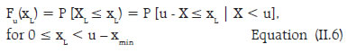 where, xmin is the smallest observation. The distribution of shortfall represents the probability that inflation (X) falls short the threshold inflation u by at most an amount XL, where, xL = u - x, given the information that X falls short of the threshold u. In terms of the underlying function, the same is as below: 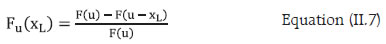 The EVT essentially considers the larger/smaller few observations of the dataset at the extreme ends and not the complete dataset. The EVT deals with conditional probabilities for example, what is the probability of inflation exceeding 25 per cent, given that it is more than 10 per cent. The challenge with EVT is determining the threshold level. Ideally, a higher threshold should be preferred. However, as the threshold increases, the modeller is left with a very small number of observations raising debatable issues on the reliability of probability estimates. Accordingly, there has to be an optimum level of threshold. There are a few standard techniques to determine the threshold statistically. One such technique is plotting the ‘Mean Excess Function’. The same is described below: If u is the threshold, the mean excess function e(u) can be estimated by the sum of exceedances (or shortfall, in case of left tail of the distribution) over the threshold u divided by the number of data points exceeding the threshold u. In other words, the mean excess function indicates the expected overshoot of a threshold given that it exceeds the threshold. For the right tail, an upward trend of the mean excess function may indicate heavy-tailed behaviour of the data; a horizontal line may suggest an exponentially distributed data, and a downward trend may indicate a short-tailed data. The underlying data may follow GPD, if the empirical mean excess function shows an upward trend, in particular, a positive gradient (upward sloping) straight line (McNeil, 1997). In our context, the mean excess plot of the data (Chart 4) is a clear upward sloping line exhibiting suitability for a Generalised Pareto Distribution (GPD) at various possible threshold points. A threshold is chosen from inspecting the plot of mean excess. Accordingly, the mean excess function is computed for our dataset 6 . It is observed that the mean excess function more-or-less maintains linearity and does not diverge across the board. This indicates that GPD may be potentially an appropriate choice for fitting the exceedances ( Chart 4). We explore and examine the appropriateness of GPD in our context and also compare it with our fitted synthetic Burr distribution. We find that the GPD is inferior to synthetic Burr, which has a poor fit at many thresholds (especially at lower u values) and has higher K-S Statistics values. The GPD appears to improve with the increase of threshold and converges with Burr though does not exhibit betterment over it. We demonstrate this for the right tail of the data (Chart 5). 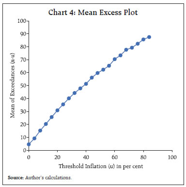 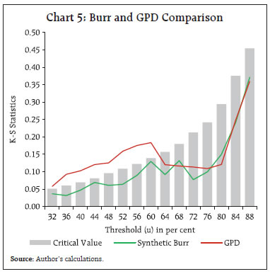 We now move to the distribution of inflation in the aggregate data. As we observed earlier (Chart 1) that the distribution of CPI-C based aggregate inflation has much shorter tails, as compared to the granular level inflation distribution. The distribution is found to be almost symmetric and platykurtic (less peaked than normal). The Log-Pearson Type III distribution is identified to be the closest representation of the aggregate level inflation data (Table 3 and Chart 6). 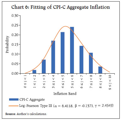 The quantile-quantile (QQ) plot exhibits a straight line highlighting the apprpriateness of the 3-parameter Log-Pearson Type III distribution for the CPI-C headline distribution (Chart 7). 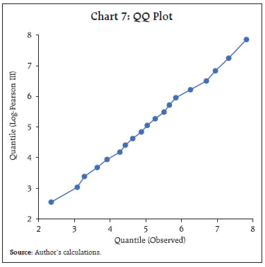 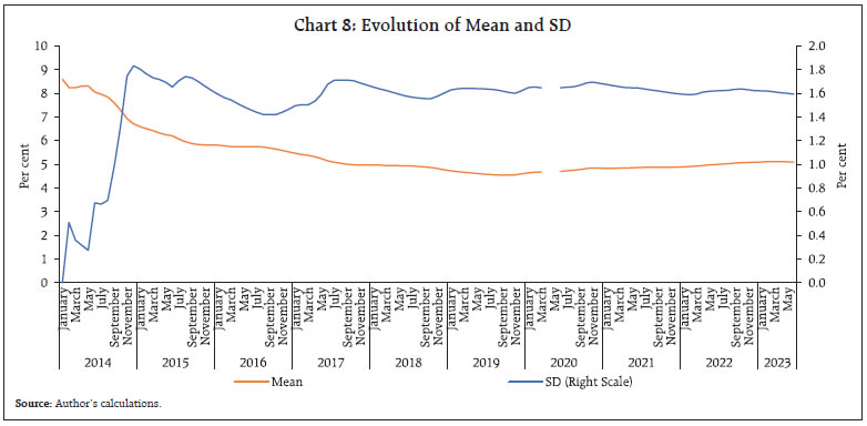 We also analyse the evolution of inflation distribution with the incoming of each incremental data point for the CPI-C aggregate data. 7 Evolution and Stabilisation of Statistical Moments of Inflation (January 2014 to June 2023) The mean inflation8 witnessed a more-or-less consistent drop since the beginning of January 2014 till September 2019, touching a trough of 4.54 per cent, which rose gradually in the subsequent period to 5.10 per cent in June 2023. The Standard deviation (SD) of the distribution appears to be settling at around 1.6 per cent (Chart 8). The skewness of the distribution dipped gradually in recent years towards zero-level, leading to a symmetric distribution. The distribution turned platykurtic (less peaked than normal) again in February 2020, just prior to COVID emergence, which remained leptokurtic (more peaked than normal) throughout December 2017 to January 2020. The unstable values of skewness and kurtosis during 2014 are due to the small sample size. Further, these do not appear to precisely converge given the current sample size (Chart 9). Now, we explore the statistical properties of inflation expectations in the following section, which is sourced from the Inflation Expectations Survey of Households (IESH) conducted by the Reserve Bank. There are other sources of inflation expectations/forecasts such as the Survey of Professional Forecasts (SPF), which is also conducted by the Reserve Bank. We restrict the analysis to IESH in the current context, as mentioned in the introductory section. III. Statistical Characteristics of the Inflation Expectations Dataset The inflation expectations survey of households is a bimonthly survey, wherein qualitative and quantitative expectations on inflation are sought from around 6,000 households 9 in select cities in the urban areas. Here, we analyse only the quantitative inflation expectations of households, which are captured from the households for three-time points - current period, 3-month ahead period and 12-month ahead period. We consider the dataset for the IESH starting from March 2014 (Round 35) to May 2023 (Round 71B) including the two bimonthly surveys conducted every year in addition to four quarterly surveys. The granular (unit) level data on inflation expectations are also released by the Reserve Bank, in addition to web releasing the summary (aggregate) data. Accordingly, we analyse both the datasets, as carried out for CPI-C based inflation in the previous section. 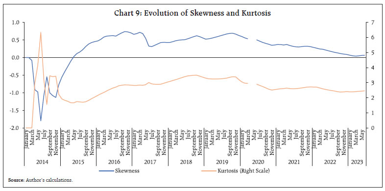 The households happen to generally report higher inflation than actual inflation. Further, there is a tendency to report higher inflation for 3-month ahead and further to 12-month ahead as compared to the current inflation (Table 4). We identify that the 4-parameter Burr distribution explains the IESH unit-level data appropriately. In the previous section, we identified that a mixture of two 3-parameter Burr distributions explains the distribution of CPI-C granular inflation well. From the IESH granular dataset, we observe that there has been a preference of households to report inflation in round numbers. This preference leads to the bunching of frequencies at round numbers and distorts the distribution. Further, unlike CPI-C granular inflation, the IESH granular inflation expectations have only one tail viz., right tail, as the lowest band (inflation less than one per cent) does not produce an extreme left tail, although it is unbounded theoretically, it is likely to be considered as between zero to one per cent by the respondents, which indeed appeared to contain a low frequency, barring 12-month inflation expectations dataset. The descriptive statistics and fitting of distribution are provided in Table 4 and Chart 10, respectively. Chart 10 exhibits the characteristics of respondents regarding their preference for round numbers, as mentioned, with round numbers in the multiples of 5, viz., 5, 10, 15, 20…..and so on. The distribution is found to be very (positively) skewed as well as very leptokurtic for all three datasets (each for current inflation, 3-month ahead inflation and 12-month ahead inflation). The 4-parameter Burr appears to pass the goodness of fit at 5 per cent though, a superior fitting may still be feasible possibly through a mixture distribution due to the inherent nature of round number preferences while responding at survey rounds. The same is not attempted in the current context though. 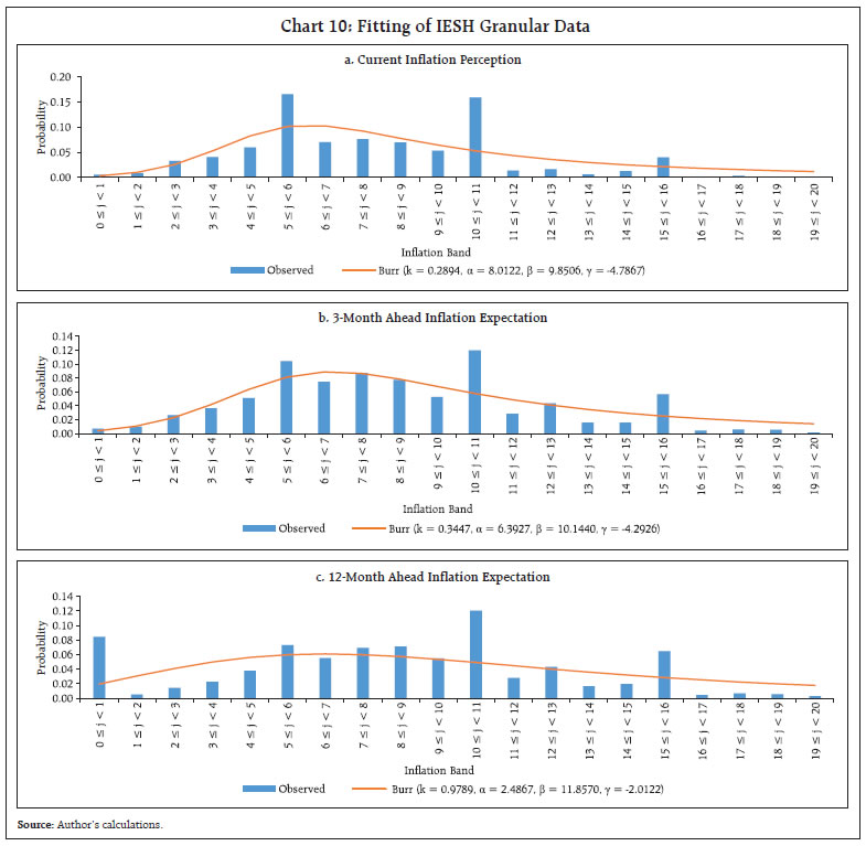 Now, we move to the fitting of IESH aggregate data. The summary statistics of the IESH data is released for two central tendencies (mean 10 and median). We identify that 4-parameter Johnson SB distribution 11 tracks the distribution of mean inflation of IESH well. The descriptive statistics and fitting are exhibited in Table 5 and Chart 11, respectively. 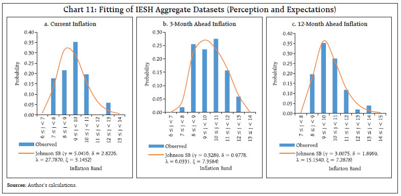 The distribution of mean inflation of IESH is found to be (positively) skewed unlike the CPI-C aggregate inflation, which was found to be almost symmetric. After studying and analysing the statistical properties of inflation and inflation expectations at the granular and aggregate level, we attempt to map these in the following section. The findings of section II and III reveal that the statistical moments of the distributions of various analysed datasets differ significantly from each other. The findings are summarized in Chart 12. The mappings, as collated in Chart 12, provide an equivalence of distribution with the other. For example, a data point of IESH (aggregate) for current inflation following the 4-parameter Johnson SB (γ = 5.0416, δ = 2.8226, λ = 27.7870, ξ = 5.1452) has a correspondence with a data point of CPI-C (aggregate) following Log-Pearson Type III (α = 6.4118, β = - 0.1371 and γ = 2.4545). The functional relationship of two datasets can be used in many ways. A simple approach is to map through the cumulative distribution function (CDF). These are potentially useful as IESH is forward-looking, whereas CPI-C realised inflation is post-facto. Accordingly, the mapping has the potential to forecast inflation. The forecast for CPI-C inflation using IESH data can be possible under two mappings – direct and indirect, as below: Direct mapping It is based on aggregate numbers and does not use granular-level information. Let X and Y be random variables representing realised inflation and 3-month ahead inflation expectations of IESH, respectively, both at an aggregate level. The mapping of a particular value ‘y’ of the 3-month ahead inflation expectation to a value of x (of realised inflation) can be done by equating FJohnson SB (y) with F log-Pearson III (x). The steps to do this mapping is given as below: 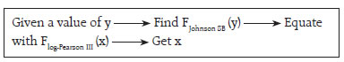 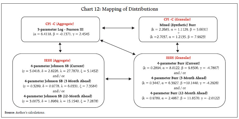 For example, the result of the 72nd round of IESH, which was conducted during July 1-10, 2023, indicated a mean of 10.20 per cent for the 3-month ahead inflation (i.e., forecast for October 2023). Using the 4-parameter Johnson SB (γ = 0.3289, δ = 0.9778, λ = 6.0331, ξ = 7.3584) distribution of 3-month ahead inflation in IESH, we compute FJohnson SB (10.20) = 0.58525. We compute x, by solving the equation, x = F-1 log-Pearson III (0.58525), wherein F-1 is an inverse CDF. This provides an estimate for x = 5.43 per cent. The above mapping could be an alternative to the traditional econometric models, which are commonly used to forecast inflation through forward-looking inflation expectations. Based on the above approach using the identified distributions with estimated parameters, we estimate the inflation for the months since March 2014, barring those months, wherein any of the two – inflation and inflation expectations are not available. We compare the estimates of inflation with realised inflation using this approach and a simple regression-based approach, an econometric tool, and observe that the proposed approach is quite competitive, which additionally provides valuable insights into the detailed profile of the datasets (Chart 13). More complex mapping of distributions could be done using Copula 12 functions, although they are not attempted in this article. Indirect mapping In direct mapping, one data point of one distribution is mapped with one data point of the other distribution, which is suitable for the aggregate dataset, as we have only one (aggregate) number per month for inflation expectations and one for the realised inflation. Instead of aggregating single numbers, we can establish a mapping between granular datasets of inflation expectations and realised inflation through many one-to-one mappings. These mappings could include the mapping of inflation at disaggregate level such as urban city (centre) of IESH versus corresponding State of CPI-C, etc. The indirect mapping could be complex and could be done in two stages, as below: 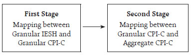 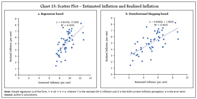 In the indirect mapping, it is feasible to analyse the distribution of incoming (new) data of a month at a granular level and compare the historical distribution (covering several months) to identify changes in the shape of the distribution, in terms of changes in moments such as skewness, kurtosis etc. This is not possible in the aggregate, being a single number. We fit the 4-parameter Burr distribution to all rounds under study on an individual basis also to get estimates of parameters of the distribution as also the round-wise descriptive statistics (Annex Table A2). We find that the mean and standard deviation of the granular level IESH data are positively correlated with the realised CPI-C inflation. The skewness and kurtosis are negatively correlated. Similarly, two parameters (α and β) appeared to be linked positively with the realised inflation, while the other two (viz., k and γ) parameters are inversely correlated. These indicators may play a useful role in econometric models as input variables aiding in forecasting inflation (Annex Table A3). The identification of one-to-one mappings in stage 1, which exhibits closer co-movement, shall be a useful exercise. The same is not explored in the current article. The second stage of the indirect mapping is expected to be stronger, being part of the same dataset. Inflation-at-Risk (IaR) The above mappings may also be useful in assessing Inflation-at-Risk (IaR) 13 . As lower inflation (left tail) has not been a concern in the Indian context, we compute IaR at 95 per cent and 99 per cent for the CPI-C aggregate data using historical (observed) inflation and using inflation expectations from IESH. The estimated distribution of CPI-C inflation i.e., Log-Pearson Type III (α = 6.4118, β = - 0.1371 and γ = 2.4545) corresponds to the inverse CDFs - F-1(0.95) and F-1(0.99) viz. the Inflation-at-Risks - IaR0.95 and IaR0.99 at 7.84 per cent and 8.84 per cent, respectively. The same using the estimated distribution of IESH i.e., 4-parameter Johnson SB (γ = 0.3289, δ = 0.9778, λ = 6.0331, ξ = 7.3584) for 3-month ahead inflation corresponds the inverse CDFs of F-1(0.95) and F-1(0.99) to IaR0.95 and IaR0.99 at 12.15 per cent and 12.70 per cent, respectively. Thus, the IaR0.95 = 12.15 per cent and IaR0.99 = 12.70 per cent of 3-month ahead inflation expectations have equivalence with the IaR0.95 = 7.84 per cent and IaR 0.99 = 8.84 per cent of realised inflation, respectively. The detailed quantile mapping of IESH current and 3-month ahead inflation along with CPI-C inflation is provided for completeness ( Table 6). Similar computations could be carried out using granular level data under the indirect mapping approach, as discussed earlier. The statistical properties of granular-level inflation and inflation expectation datasets remain important and can be analysed through suitable statistical distributions. This article attempts to map the datasets of survey-based inflation and actual inflation through their long-run statistical distributions, which appear to be an unexplored area of research. The variants of Burr distributions are found to be appropriate in explaining statistical characteristics of both the granular level datasets, viz. survey-based inflation expectations and the realised inflation. The aggregation of these datasets provides useful summary statistics such as headline inflation numbers. As the survey-based inflation expectations are forward-looking and have been useful in forecasting inflation for the short-term for which econometric tools are widely used, the functional relationship through suitable statistical distributions derived in the article may facilitate short-term forecasting as a non-econometric tool. Further, the roun-dwise estimated parameters for the survey-based inflation expectations may also be used as an input to the suitable econometric models. The identified distributions can also be used to measure Inflation-at-Risk for the observed inflation and survey-based inflation expectation datasets. References Andrade, P., Ghysels, E. and Idier, J. (2012), “Tails of Inflation Forecasts and Tales of Monetary Policy”. Working Papers, Banque de France. Carreau, J. and Bengio, Y. (2009), “A hybrid Pareto model for asymmetric fat-tailed data: the univariate case”, Extremes 12, 53-76. Cooray, K. and Ananda, M. M. A. (2005), “Modelling actuarial data with a composite Lognormal-Pareto model”, Scandinavian Actuarial Journal (5), 321-334. Das, A., Lahiri, K. and Zhao, Y. (2019), “Inflation expectations in India: learning from household tendency surveys”. International Journal of Forecasting, 35 (3), 980-993. Frigessi, A., Haug, O. and Rue, A. (2002), “Dynamic mixture model for unsupervised tail estimation without threshold selection”, Extremes, 5, 219-235. McNeil, A. J. (1997), “Estimating the tails of loss severity distributions using extreme value theory”, ASTIN Bulletin, Vol. 27, No. 1, 117-137. Muduli, S., Nadhanael, G. V. and Pattanaik, S. (2022), “Assesing inflation expectations adjusting for households’ biases”, Monthly Bulletin, Reserve Bank of India, December. Nadarajah, S. and Bakar, S. A. A. (2014), “New Composite Models for the Danish Fire Insurance Data”, Scandinavian Actuarial Journal, 2, 180-187. Salido, D. L. and Loria, F. (2021), “Inflation at Risk”, Federal Reserve Board, September 08. Sastry, D. V. S. and Sinha, R. K. (2010), “A Revisit to Danish fire loss data”, Conference Proceedings, 12th Global Conference of Actuaries (GCA), Mumbai, India. Scollnik, D. P. (2007), “On composite Lognormal-Pareto model”, Scandinavian Actuarial Journal, Vol. 2007, Issue 1/2007, 20-33. Scollnik, D. P. and Sun, C. (2012), “Modelling with Weibull-Pareto models”, North American Actuarial Journal, 16 (2), 260-272. Shaw, P. (2019), “Using rational expectations to predict inflation”, Reserve Bank of India Occasional Papers, Vol. 40, No. 1. Sinha, R. K. (2023). “India’s Steady State Equilibrium Inflation: A Revisit”, Monthly Bulletin, Reserve Bank of India, May. 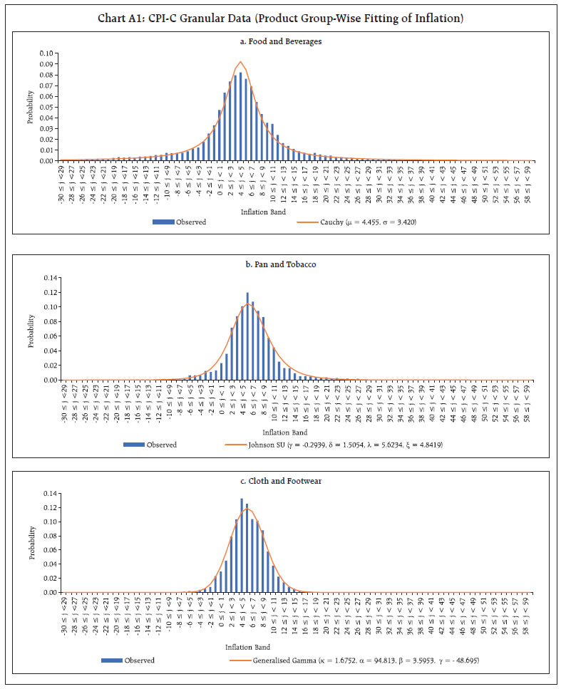 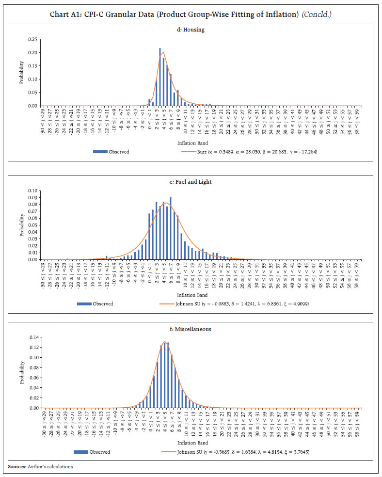
^ The author is from the Monetary Policy Department (MPD). The views expressed in this article are those of the author and do not represent the views of the Reserve Bank of India. 1 The comparative study is also possible using the information on inflation expectations of other respondents such as professional forecasters. The same is not explored in this article. 2 The study considers 22 larger States/UTs, which have individual weights of more than 0.25 per cent in the CPI-C basket. These States collectively cover 98.30 per cent of CPI-C basket and have greater level of granularity as compared to the set of smaller States. 3 The probability density function of the disaggregate and aggregate inflation data would be different though the central tendency derived from these two datasets would be comparable. However, other statistical moments of the data (viz., standard deviation, skewness and kurtosis) may differ significantly. For example, the standard deviation of the granular data would be higher than that of the aggregate data. 4 Dagum distribution is the inverse of Burr distribution, which is used to fit heavy tailed distributions. 5 The appropriate weights of the left and right tails are derived from the observed data at around 0.41 and 0.59 (Table 2). 6 We use probability weighted counts of observations in our context to reflect varied and appropriate weights of the products/sub-products. This is unlike many other studies, wherein simple counts are applied to derive mean excess function, which is meaningful in loss distributions such as Danish fire loss dataset, demonstrated by many studies. 7 The evolution and stabilisation of granular-level data of CPI-C based inflation was discussed in the study (Sinha, 2023) covering the pre-COVID and post-COVID periods with additions of half-yearly data. The study found a consistent right-ward shift in the distribution in the post-COVID period. 8 The mean inflation at a month (t) is a simple average of inflation starting from January 2014 to the month (t). 9 The number of surveyed households has increased in recent times with the introduction of new cities/centres for the survey. 10 The published mean of the IESH may not match with the mean computed from the granular level data due to various aggregation and methodological issues. 11 Johnson System Bounded (SB) distribution is a system of curves for bounded data, which can be transformed to an approximately normal distribution through an appropriate transformation function. Similarly, Johnson System Unbounded (SU) distribution is a system of curves for unbounded data, which is found to be suitable in this study for select product groups in the CPI-C granular dataset ( Annex Table A1). 12 Copula is a multivariate cumulative distribution function for which the marginal (individual) probability distribution of each variable is uniformly distributed in the interval [0, 1]. It models the dependence (inter-correlation) structure between random variables and is widely used in financial datasets. 13 There are different approaches to define and measure Inflation-at- Risk (IaR). IaR was originally introduced by Andrade et al. (2012) to assess the risks to the inflation outlook. The study constructed a Value-at-Risk (VaR)-type measure of tail risk for inflation using survey-based conditional density forecasts. They observed that the magnitude and the asymmetry of inflation risks varied over time. A recent study by Salido and Loria (2021) used a probability-type measure for IaR. It also highlighted importance of skewness in the IaR. In the current context, we use a simple VaR-type measure for IaR. |
|||||||||||||||||||||||||||||||||||||||||||||||||||||||||||||||||||||||||||||||||||||||||||||||||||||||||||||||||||||||||||||||||||||||||||||||||||||||||||||||||||||||||||||||||||||||||||||||||||||||||||||||||||||||||||

हे पेज शेअर करा:


भारतीय रिझर्व्ह बँक मोबाईल ॲप्लिकेशन इंस्टॉल करा आणि नवीनतम बातम्यांचा त्वरित ॲक्सेस मिळवा!
आमचे अॅप इंस्टॉल करण्यासाठी QR कोड स्कॅन करा


पेज अंतिम अपडेट तारीख:


