 IST,
IST,


RBI WPS (DEPR): 08/2023: Portfolio Flows and Exchange Rate Volatility: An Empirical Estimation for BRICS Countries
| RBI Working Paper Series No. 08 Portfolio Flows and Exchange Rate Volatility: Dipak R. Chaudhari, Pushpa Trivedi and Prabhat Kumar@ Abstract * This paper examines whether foreign portfolio flows are responsible for exchange rate volatility in the BRICS economies. Applying the GARCH (1, 1) model to monthly data from January 2000 to July 2021 on exchange rate returns, this paper finds that net portfolio flows in bond and equity markets impact exchange rate returns and volatility in the returns of the BRICS currencies. However, the BRICS countries have been successful in reducing currency volatility through foreign exchange market interventions. Further, net inflows are associated with appreciation in the BRICS currencies, except for that of Brazil during the post-GFC period. JEL Classification: F31, F32, G15 Keywords: Portfolio flows, bond, equity, exchange rate volatility, BRICS countries, currency appreciation, GARCH (1, 1), granger causality Introduction Globalisation plays a major role in the modern economic development. Product innovations and advancements in information and technology have upgraded humankind's living standards. Greater global financial integration has resulted in increased international trade in goods and services, labour force migration for better employment and capital flows for optimal use and higher returns. However, globalisation can also lead to financial instability and associated losses of output and employment (Pattanaik, 2001). The inflation pass-through via exchange rate can also introduce volatility in commodity prices (Ndou et al., 2019). An increase in cross-border capital flows is believed to be an important factor in increased volatility in exchange rates (Caporale et at., 2017). Capital flows are broadly categorised into foreign direct investment (FDI) and foreign portfolio or institutional investment (FPI or FII).1 With the gradual opening of the economies around the globe, investors have got an opportunity to invest in other countries to maximise their returns, leading to an increase in cross-border FPI flows. In the US, cross-border FPI transactions in bonds and equities markets were 4 per cent of its GDP in 1975 which increased to 245 per cent by 2000 (Hau and Rey, 2006). The growth in FPIs has been much more than FDI flows. FPI flows are considered to be most volatile, sometimes called ‘hot money’ (In-Mee Baek, 2006) as these flows are motivated purely by returns and are susceptible to economic outlook. The speculative nature of the FPI flows, sudden inflows and outflows can create volatility in the emerging market economies (EMEs). By contrast, FDI is influenced by economic fundamentals and tends to be less volatile (Uctum and Uctum, 2011). Rafi and Ramachandran (2018) examined currency volatility in EMEs and observed that the FPI flows contributed more than 7 per cent to the exchange rate volatility in these economies. In deciding about the policies related to FPI flows, emerging economies may account for the impact of these flows on exchange rate variability (Rafi and Ramachandran, 2018). Exchange rate movements in turn can influence international trade. An appreciation in domestic currency can adversely impact exports as domestic goods become more expensive while depreciation can make them cheaper. Multinational companies are reluctant to trade with a country whose exchange rate is volatile. Finally, exchange rate volatility can affect the financial system, making monetary policy objectives more difficult to achieve. In August 2013, Morgan Stanley created a term “Fragile Five”2 to symbolise EMEs which had become too reliant on unreliable foreign portfolio flows to finance their economic growth aspirations. Against this background, this paper analyses the implications of FPI flows for exchange rate volatility in the BRICS economies. Studies in this area mainly focus on advanced economies (AEs) (Caporale et al., 2017). There are very few studies in the context of emerging economies. The BRICS group consists of a) a large population along with large-scale production; b) a major economic block accounting 22 per cent of gross world product; c) a significant share in emerging market equities value; and d) various fund managers that have set up dedicated BRICS investment funds. In sum these economies, as they transit from developing to developed countries, are important for economic research (Collins, 2005). To understand the linkage between portfolio flows in debt and equity markets to the exchange rate volatility, the paper uses econometric approach of Generalised Autoregressive Conditional Heteroskedasticity (GARCH) estimation technique developed by Bollerslev (1986). The rest of the paper is organised into the following sections. Section II undertakes a survey of literature on the exchange rate volatility and portfolio flows. Section III presents stylised facts related to BRICS and the selected variables. Section IV explains the data and the methodology. Section V concludes by providing a summary and findings of the study. The literature gives vital importance to understanding the empirical relationship between foreign capital flows and nominal exchange rates. Dornbusch (1980) has argued that exchange rate adjusts instantaneously to clear the asset market while other asset classes adjust steadily. Bonser-Neal (1996) provided three main reasons for exchange rate volatility – first is the change in market fundamentals, including income, interest rates, productivity, and money supply, second is the change in future expectations of economic fundamentals and policies; and third is the change driven by speculators/hedgers. Most of the previous studies on the linkages between exchange rates and FPI flows focus on the advanced economies. Hau and Rey (2006) empirically estimated the relationship between exchange rates, equity prices, and capital flows using multiple frequency data (daily, monthly, and quarterly) for 17 OECD (Organisation for Economic Co-operation and Development) countries in comparison with the US. The authors found that portfolio flows were closely associated with changes in exchange rates, and net equity flows were positively interrelated with appreciation in foreign currency. Ali et al. (2014) analysed the effect of bond and equity portfolio flows on exchange rate volatility using two-state Markov-switching models for Canada, countries in the European Union, Japan and the UK. The authors found that the relationship between net portfolio flows and exchange rate volatility was non-linear for all currencies, excluding the Canadian dollar. In the case of Canada, net portfolio inflows are not found to be impacting the exchange rate volatility. The same group of authors extended the analysis for the US against Australia, Canada, the European Union, Japan, Sweden, and the UK from January 1988 to December 2011 (Caporale et al., 2015) and observed that the effect of exchange rate uncertainty on net equity flows is negative in the Euro area, the UK and Sweden. However, it was positive in the case of Australia. Overall, the findings suggested that any type of portfolio flows (bond or equity) heightened exchange rate uncertainty in the receiving country and led to financial instability. Using the VAR model, Froot et al. (2001) analysed the relationship among net portfolio flows, equities and currency returns. The authors observed a positive and contemporaneous relationship between net portfolio inflows and lagged equity and currency returns for 44 countries. Similarly, Brooks et al. (2004) observed that the portfolio outflows from the euro area to the US led to Euro depreciation against the US Dollar. While Siourounis (2003), using monthly data and applying an unrestricted VAR model, found that portfolio equity flows rather than portfolio bond flows impacted the exchange rates dynamics from 1988 to 2000 for USD vis-à-vis the Pound, Yen, Deutsche Mark and Swiss Franc. In comparison to AEs, there are a few country-specific studies on EMEs, such as for Turkey (Uctum and Uctum, 2011) and South Africa (Frankel, 2007). Most studies relating to EMEs include a group of these countries, such as Combes et al. (2012) for 42 economies, Ananchotikul & Zhang (2014) for 17 economies, Caporale et al. (2017) for Asian EMEs, In-Mee Baek (2006) for Latin American economies and Aydoğan et al. (2020) for six EMEs. Combes et al. (2012) examined the long-run cointegrated inter-relationship between capital flows, exchange rate flexibility and the real effective exchange rate for 42 advanced and emerging economies from 1980 to 2006. The authors found that all capital inflows were associated with an appreciation of the real effective exchange rate. Among the various capital flows, portfolio inflows had the most significant impact on the appreciation of the currencies. Ananchotikul and Zhang (2014) examined 17 emerging economies and found that global risk aversion is a major factor impacting exchange rate volatility. However, the magnitude of the impact was more dependent on country-specific characteristics, such as financial openness of the economy, the exchange rate framework, and other macroeconomic variables like inflation, current account balance, etc. In line with findings of the other studies, the authors confirmed that portfolio flows impact exchange rate returns. Although the representation of EMEs in the literature is limited, these economies offer interesting cases for understanding the relationship between capital flows and exchange rate volatility because they are at different stages of openness in terms of their regulatory framework, restrictions, sectoral caps, etc. Hence, exchange rates may respond differently depending on the size of the economy and the volume of flows in EMEs. A major obstacle in studying portfolio flows into EMEs is the lack of data availability. Very few developing countries provide segment-wise portfolio investment data. Usually, researchers source portfolio flows data from US Treasury International Capital (TIC) system, which has various limitations described by Caporale et al. (2017). Further, the data on net portfolio flows taken from the US TIC System covers only transactions involving US residents. Another data source for cross-country FPI flows is IIF (Institute of International Finance) dataset, which is comparable with the IMF and World Bank database as it follows balance of payments-based methodology. Yet another data source is the EPFR dataset (https://epfr.com/), which covers portfolio flows related to the mutual fund industry and exchange traded funds, as a subset of the overall portfolio flows (Ananchotikul and Zhang, 2014). Among the studies focusing on the BRICS economies, Altunöz (2020) evaluated the dynamics of net portfolio flows in bond and equity and exchange rates for India, Brazil and Russia. The author sourced the portfolio flows data from US TIC System for the period 1997 to 2017. Using non-linear two-state Markov switching specification, the author got mixed results. He found that the net bond flows led to an increase in exchange rate volatility in Russia. However, there was no impact seen in the case of Brazil. Overall, the author found that net equity flows from emerging economies to the US led to an increase in volatility in domestic exchange rates. While studying the BRICS and other economies, Aydoğan et al. (2020) examined the role of portfolio flows in the exchange rate volatility in Brazil, Russia, India along with Indonesia, Mexico and Turkey. The study found a correlation between the overall portfolio flows and exchange rate volatility. On the other hand, portfolio flows in the bond market, and the correlation was only in the case of Brazil and Mexico. These results indicated that portfolio flows in bond and equity markets were country specific. Gautam et al. (2020) evaluated the relationship between exchange rates and capital flows in the BRICS countries for the period 1994:Q1 to 2019:Q2. The authors employed the ARDL bound technique and found a positive relationship among the BRICS exchange rates. Kodongo and Ojah (2012) examined the relationship between net foreign portfolio flows and exchange rates in the major countries of Africa. The authors used monthly portfolio flows data from IIF for 1997:M1 to 2009:M12. Their findings of Granger causality test did not suggest any direction of causality between exchange rates and net portfolio inflows. However, in the case of South Africa, the authors found a bi-directional causality between exchange rate and portfolio flows. International capital flows are also dependent on the exchange rate regime and openness of the economy. Jiang (2019) provided a comparative analysis of the exchange rate regimes in the BRICS countries and found that Brazil was the only country with a free-floating exchange rate system among BRICS countries. In contrast, the other four countries followed a managed float exchange rate system, though with some differences. In the case of India, many studies have explored the relationship between foreign capital flows and exchange rate volatility. RBI (2021) analysed the drivers of INR-USD volatility for the period 1996:Q2 to 2019:Q4 using vector auto-regression framework and found the FPI flows to be most volatile among different instruments of capital flows. However, it also found that the INR-USD volatility reduces with an increase in net FPI inflows. By contrast, the other types of capital flows increased the INR-USD volatility. Kohli (2015) evaluated the role of FPI flows and other macroeconomic variables in determining the INR volatility. Using generalised method of moments, the author observed that financial openness and gross portfolio flows were major external factors impacting rupee volatility. Furthermore, after replacing net portfolio flows with gross flows, the author observed that the flows reduce exchange rate volatility in the short-term. Dua and Sen (2013) examined the relationship between real exchange rate and volatility of capital flows between 1993 and 2010. The authors identified that net capital inflows and their volatility jointly impacted INR-USD exchange rate. Further, the findings suggested that capital inflows appreciated the exchange rate, resulting in a huge trade deficit. BRICS is a dominating group in international trade and finance. Regarding the size of these economies, China dominates with a GDP of USD 14.7 trillion followed by India having a USD 2.6 trillion economy. Brazil and Russia have a similar economic size of USD 1.4 trillion while South Africa’s GDP is USD 0.3 trillion. In terms of foreign trade, China dominated the group with USD 2.59 trillion exports in 2020 (Table 1).
The BRICS countries started with divergent merchandise trade growth. The growth was 5.8 per cent for South Africa and 27 .6 per cent in the case of Russia. However, in recent years, they have come to compete very closely, and the growth rates during 2015-2020 are seen to be converging (Table 2). Russia and China are current account surplus economies while other countries have mostly experienced deficit in their current accounts. However, South Africa, India and Brazil were able to reduce their current account deficits which has resulted in an increase in investors’ confidence. For Russia, although current account deficit is not a problem as the country has maintained surplus mainly due to higher commodity prices, its main concern has been Ruble volatility that has increased due to geopolitical tensions between 2014 and 2022, including the recent conflict involving Ukraine (Chart 1). 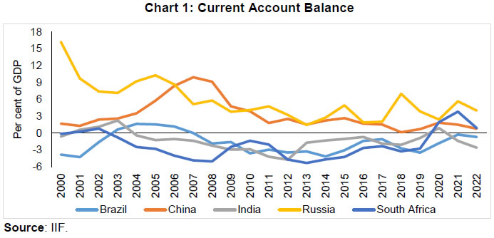 The BRICS countries adopted liberalised economic policies around the same time, and gradually allowed foreign portfolio investments into their domestic markets. In 1991, Russia enacted the first law to allow foreign investment in domestic market. In 1991-92, Brazil enacted a series of legislations to provide access to FPI flows. In 1998, India allowed FPI flows in the corporate bond market. In 1994, South Africa ended Apartheid and implemented reforms related to foreign investments. In 1995, China liberalised foreign investment in their mainland, and in 1996, it embarked on current account convertibility. The chronology of major policy changes related to the FPI flows in the BRICS countries are tabulated in Annex Table A.1. 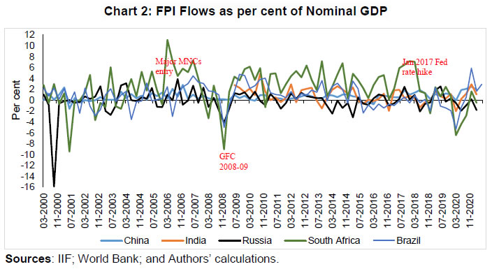 It has been observed that the BRICS countries are competing among themselves due to the commonalities and the competitive growth potential. The high economic growth over the past two decades of the BRICS countries has resulted in higher FPI inflows. However, the inflows have been volatile, ranging from (-)17 to (+)10 per cent of their GDP, respectively (Chart 2). Learning from the Global Financial Crisis of 2008-09, many central banks started to moderate portfolio flows to curb exchange rate volatility (Mohanty and Berger, 2013). The sensitivity of the portfolio flows to the global events has been more severe for countries with current account deficits. During the COVID-19 pandemic, the portfolio flows declined sharply and then bounced back. The increase in the portfolio flows towards emerging economies could be attributed to the easy monetary policies adopted by the US and other advanced economies. When market was in a boom phase, portfolio flows shifted to emerging market economies in search of high returns, while the reverse happened during periods of increased risk aversion. This resulted in high volatility and not necessarily reflecting domestic macroeconomic fundamentals. As a preliminary attempt to understand the relationship, simple correlations were worked out between exchange rate returns and net FPI flows. The negative correlation for all five countries indicated that any kind of FPI flows create appreciation pressures on the domestic currency (Table 3). The results were in line with the findings in the literature (Hau and Rey, 2006). Here, return has been defined in terms of the log return, i.e.,  Here, Et is domestic exchange rate per USD. Any change in the foreign exchange market directly or indirectly impacts the economy through various channels, like exports and imports, capital flows, and external borrowings. A stable exchange rate lowers the risk for exporters and importers, increases international trade, and improves the growth potential, by making it easy for an entrepreneur to work on future projects and investments. Thus, ensuring orderly conditions in domestic forex market is the primary concern of policymakers. It has been observed that during the Global Financial Crisis and Taper Tantrum, exchange rate movements in BRICS countries were high resulting in heavy interventions by the central banks of these countries to stabilise their exchange rates (Annex Chart A.1). After the balance of payments crisis in 1999, the Brazilian economy underwent many institutional reforms, including changes in the monetary policy framework. In 1999, the Brazil Central Bank (BCB) adopted the inflation targeting (IT) framework and a floating exchange rate regime. Despite the floating exchange rate regime, BCB intervenes in the market more frequently and publishes intervention data on a daily basis. Among BRICS central banks, BCB is unique in terms of intervention. To illustrate, it invested around USD 50 billion in 2012-13 as interventions in the onshore derivatives market (Garcia, 2013). Bank of Russia (BoR) has gradually shifted its focus from exchange rate targeting to the inflation targeting in 2015. To smoothen exchange rate volatility, the BoR intervenes in the foreign exchange market with the buying and selling of USD and Euro. During the Global Financial Crisis of 2008-09, when Ruble volatility was high, the BoR intervened heavily and sold foreign currency. Further, during the Russia and Ukraine conflict in 2014, the Ruble experienced an all-time high volatility. Like other BRICS’ currencies, the INR also experienced high volatility during the GFC period. However, in comparison to GFC, the magnitude of volatility was quite high during the Taper tantrum episode in 2013. The Chinese Yuan has been comparatively stable among the BRICS’ currencies mainly as the Yuan was pegged with US dollar up to July 2005. As per the official statements from the People’s Bank of China (PBOC), it now has a managed floating system with reference to a basket of currencies. Further, the PBOC has claimed that Renminbi (RMB) is market determined. The PBOC had a fixed daily band of RMB/USD +/- 0.3 per cent from 2005 to 2007. Subsequently, the band widened to +/- 0.5 per cent from 2007 to 2012 and 2 per cent up to 2014. On August 11, 2015, the PBOC surprised market by consecutive three times devaluation of the RMB, reducing its value by 3 per cent against USD. Regarding currency intervention, China has frequently used exchange rates to benefit its export-led economic growth. On the intervention issue, the US treasury has often labelled China as a “currency manipulator”. Since January 2020, however, the US Treasury lifted its description for China as a currency manipulator. The Phase One Trade agreement between China and the US required changes to the former’s policies and practices in several key areas, including currency issues. In this settlement, China had made upfront commitment to refrain from devaluation of its exchange rate to boost exports. Historically, the South African Reserve Bank (SARB) has intervened in the foreign exchange market in both spot and derivative markets. The overall objective of the SARB’s intervention operations is not to manage the exchange rate but to keep it competitive against its trading partners. Its other objective is to build up foreign exchange reserves. IV.1 Methodology To study the impact of portfolio flows in bond and equity segment on the BRICS’ currencies, we have followed Caporale et al. (2017) and used log returns of exchange rate as the dependent variable. The log returns are calculated as: 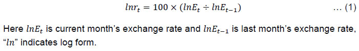 The conventional ordinary least square (OLS) models assume – homoskedasticity (expected values of all error terms are same at any point). However, exchange rate returns, and volatility in the returns follow heteroskedastic pattern (Huang et al., 2011) – the variance in the error terms are different at any given time, called as time-variant variance. Further, the variance shows “volatility clustering”, where “large changes tend to be followed by large changes, of either sign, and small changes tend to be followed by small changes”, meaning that there are periods of low and high volatilities in the sample. This “clustered volatility” is termed as autoregressive conditional heteroscedasticity (ARCH) in the literature. Conditional heteroskedasticity is an interesting property because it can be exploited for forecasting the variance in future periods. In the presence of heteroskedasticity, the regression coefficients for an OLS regression are still unbiased. However, the standard errors and confidence intervals estimated by OLS regression will be small and may provide a false sense of accuracy. Hence, considering the heteroskedastic nature of the data, we have used the ARCH and GARCH models. The ARCH and GARCH treat heteroskedasticity as a variance to be modelled. The model describes the variance of the current error term as a function of the actual sizes of the previous periods' error terms. The baseline econometric model has the following specification:  Here, 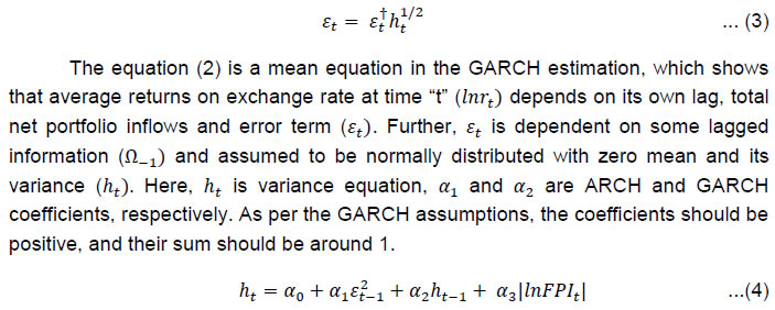 Further, as the FPI flows are of two types, bond and equity, they are of different nature and impact the exchange rate returns and volatility differently. To understand the effect of bond and equity flows impact on exchange rate volatility, we have examined the following equation:  In the equation (5), bond and equity flows are taken separately and also the variance equation (eq. 7) has been changed accordingly.  In the variance equation (ht), expected signs for α1 and α2 are positive and if both are combined, the value should be around 1. The | | is absolute value of variance. In time series analysis, the first stage of any empirical investigation is to check the stationarity of data. The paper uses Augmented Dickey Fuller (ADF) test for the stationarity check. The ADF test is based on the idea of testing whether the coefficient of lagged values of time series is equal to one i.e., presence of unit root. Therefore, the null hypothesis is that the series has unit root implying non-stationarity. Furthermore, considering the various other factors impacting exchange rate simultaneously, we have extended the empirical analysis by adding other variables in the above equation - Central bank intervention and interest rate differential. Although the common motive behind intervention is to reduce exchange rate volatility, empirical evidence of effectiveness of intervention are mixed. As per the central banks’ stated policies, all BRICS central banks use intervention as a major policy instrument to curb volatility. The difference between US yield and BRICS countries yield can be a major factor impacting exchange rate volatility. However, literature does not provide any unanimous view in this connection. Brooks et al. (2004) found that interest rate was not the crucial factor in USD-Yen exchange rate determination post 2000. Further, during the Taper tantrum episodes of 2013, when many countries including India were witnessing massive capital outflows, Pakistan witnessed inflows. It was ascribed to the high interest rate offered on Pakistan securities. Hence, to understand the effect of intervention and interest rate differential along with bond and equity flows, we have examined the following equations: 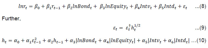 IV.2 Data Description For our analysis, the dependent variable is the nominal exchange rate, exchange rate per US dollar of the respective currency. The study is based on monthly data on bonds and equity flows and exchange rate per US dollar (end of the month) for the period January 2000 to July 2021. The data on exchange rate are taken from International Monetary Fund (IMF)’s International Finance Statistics (IFS). The rationale for taking end-of-the-month exchange rate, rather than the monthly average, is to understand the impact of portfolio flows of the month on the exchange rate. As portfolio flows are volatile varying on a day-to-day basis, taking the average of the monthly exchange rate may not be appropriate to gauge the impact on these flows. Bond and stock portfolio flows data are obtained from the Institute of International Finance. The IIF is an international organisation of market participants and policymakers including central banks, investment firms and financial institutions from 70 countries. As the dataset follows balance of payments-based methodology and constructed using country-wise individual country data sources, it is comparable with the IMF or World Bank database. Based on the literature (Ishii et al., 2006), the study uses an interest rate differential variable. This is the difference between home country and the US 10-year government securities yield. The data is sourced from the OECD database. The motive behind choosing the interest rate differential variable is to capture possibly the US monetary policy spillover effect on local currency. In our dataset, a positive interest rate differential between BRICS counties against the US indicates the possibility of ‘carry trade’ involving borrowing in low interest and investing in a high-interest market. These observations are in line with the interest rate parity theory. We observed sudden jump in the Russian interest rate differential in the year 2014-15 due to the currency crisis faced by the country. China’s interest rate differential is mostly around zero proving the resilient nature of the economy against the US economy. In the BRICS countries, actual intervention data is available only in the case of Brazil, Russia and India. Among these, Brazil publishes on a daily basis, while Russia and India publish on monthly frequency with around 2-month lag. It is a daily frequency for Brazil, while it is a monthly frequency for Russia and India. South Africa and China do not publish intervention data. In this background, we have used a database recently published in an IMF working paper (Adler et al., 2021). The data on intervention is calculated as a per cent of GDP. We have used log of all the selected variables. However, all the data series are not always positive as sometimes exchange rate intervention can be negative due to the sale of foreign currency. The interest rate differential between home country and the US can be negative also. Hence, considering the common practice in the literature (Herrmann and Mihaljek, 2013; Karakaplan et. al., 2020; Behera and Mishra, 2020; and Shankar 2002), we have added a constant value to the series. A constant is a maximum negative value in the series to make the series non-negative. Adding a constant neither changes parameter estimates nor the parameter as coefficient of variation is standardised and unit free measure. By examining the contemporaneous correlation matrix, it has been observed that the returns of the BRICS economies are positively correlated. The positive correlation among BRICS currencies indicates that the returns are competitive (Table 4). The other variables are foreign portfolio investment in bond market and equity market- indicated as “lnBond” and “lnStock” respectively. The other variable is “lnFPI”, which is net FPI flows (Bond + Stock) (descriptive statistics are given in Annex Table A.2). The descriptive statistics indicates that for the sample period, i.e., January 2000 to July 2021, returns on BRICS’ currencies were positive indicating depreciation against the US dollar, except Chinese Yuan, which was negative showing appreciation against the US dollar. Also, the standard deviation of returns on Yuan was less than the other currencies indicating relative stability of the currency among others. Positive skewness and high kurtosis suggest potential high gain with low degree of probability in the foreign exchange market. Kurtosis value for portfolio flows in bonds, stocks and overall FPI showed positive values implying their ‘hot money’ character. In order to avoid spurious regression, it is important to carry out a stationary test. The stationarity is a property of data with constant mean and constant covariance. In other words, series need to be stationary to avoid spurious regression. For this purpose, the Augmented Dickey-Fuller (ADF) test has been used, adjusting for serial correlation. The ADF test results suggest that all the select variables are I(0), indicating that all our variables are stationary at level (Annex Table A.3). Further to understand the relationship between exchange rate volatility, FPI flows (both in bond and equity) and central bank intervention, we carry out Granger causality test (Table 5). As expected, the null hypothesis that FPI flows do not Granger cause exchange rate volatility is rejected in the case of Russia, India and China. However, for Brazil and South Africa, we did not get significant F-statistic values. The null hypothesis that volatility does not granger cause intervention is rejected in the case of India and China. As the granger causality results are inconclusive and country-specific, we proceed to our GARCH estimation of the association between FPI flows and exchange rate returns. IV.3 Empirical Results We estimate the baseline equations (2) to (4) using GARCH (1,1) framework developed by Baillie & Bollerslev (1989) (Table 6). 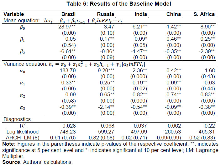 The estimation shows that the dataset is suitable for the GARCH framework. The statistically significant coefficients for all BRICS countries (except Brazil) [β1, which is return on exchange rate (-1) in the mean equation] indicates that past exchange rate values can largely decide the present value of the exchange rate return. The significant coefficients of β2 in case of all the countries indicates that the foreign portfolio flows are impacting the level of the returns on the exchange rate. ARCH and GARCH terms (α1 and α2 respectively) in the variance equation are statistically significant (except for South Africa where only the GARCH term is statistically significant), and both coefficients are positive and are close to one (1) indicating presence of ARCH and GARCH effects in the model. The FPI coefficients in all these countries are found to be statistically significant and negative, pointing out that net FPI inflows reduce volatility in the returns. The interpretation of this sign can be ambiguous - rooted on the already mentioned granger causality test. Again, one possible interpretation could be that in the dynamic forex market FPI inflows, central bank interventions can be simultaneous. We have tested the residual diagnostics for all five countries and found that the residuals and squared residuals are not serially correlated and have no heteroskedasticity in ARCH-LM test. Further, following Meese and Rogoff, (1983) the RMSE values have been compared with a random walk model for all five BRICS country cases. It has been observed that all the RMSE values of the model are lower than its counterpart of random walk models (Annex Table A.4). Hence, it is reasonable to conclude that the model offers a good fit. Moving to the estimation results of equations 5 to 7, we observed that FPI flows – both in bond and equity – have statistically significant coefficients for all the BRICS countries (except Russia for bond flows) (Table 7). Further, all the β3 coefficients signs are negative indicating equity flows are creating appreciation pressure on the domestic currencies. In the variance equation, both ARCH and GARCH terms are statistically significant (except South Africa, where only GARCH term is significant) and close to one, indicating that once volatility is high, it remains high for a long period. Further, the bond and equity coefficients are statistically significant indicating both types of FPI flows have an impact on exchange rate volatility in the returns. The negative coefficients of bond flows for Brazil and South Africa indicate that the FPI flows in bond segment reduce volatility in returns. However, in the case of India the sign is positive, reflecting that the bond flows increase volatility in the exchange rate returns. The equity flows coefficient is positive for Brazil and South Africa, indicating that equity flows increase volatility in the exchange rate returns whereas the coefficients are negative in the case of Russia, India and China signifying that equity flows reduced volatility in the returns. 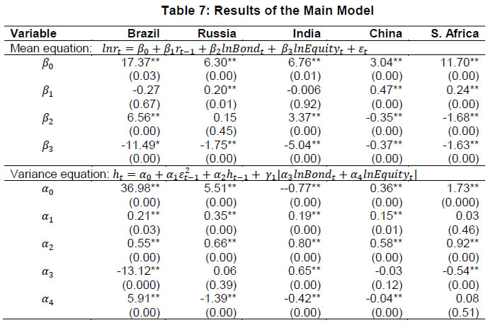 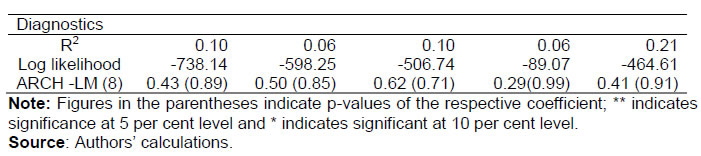 The results of the residual diagnostic tests show that the model is a good fit for the estimation. The adjusted R-square values range from 0.06 to 0.21, indicating the model explains 6 per cent to 21 per cent variation in exchange rate returns. The negative signs of the bond flows in Brazil, South Africa and equity flows in Russia, India and China indicate that the flows are reducing volatility in the exchange rate returns, which contradicts the common perception of portfolio flows increasing volatility. Hence, considering the results may be due to omitted variables bias issue, we re-estimate the model with additional variables - intervention and interest rate differential (Table 8). The results show that the additional variables increase predictive ability of the model. Here, we have added two new variables - central bank intervention and interest rate differential capturing difference in domestic and US interest rates. As all the five BRICS central banks undertake interventions to avoid volatility in their exchange rate, the intervention variable is crucial (Neely, 2008). The interest rate differential can also be the driving factor for FPI flows as higher interest rate differential fetches them higher returns. However, the results are mixed for intervention and interest rate differential, the impact of bond and equity flows on exchange rate returns (create appreciation pressure on domestic currency) remains same as it was in the earlier models in the mean equation. The intervention coefficient is statistically significant and carries a negative sign for India and China indicating that intervention reduces returns in the exchange rate. For Brazil, the positive sign for interest rate differential suggests that difference between domestic and US interest rates depreciates Brazilian Real. 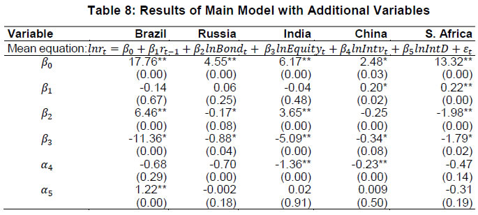 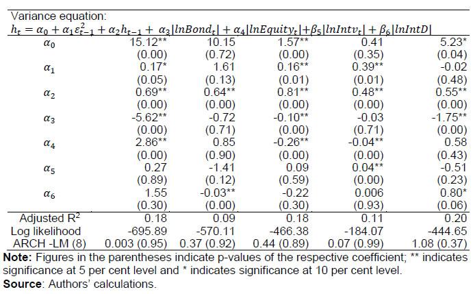 In the variance equation, GARCH coefficients are statistically significant and less than one for all BRICS countries, indicating the suitability of the model. However, the negative signs of bond and equity coefficients of BRICS countries remain the same as in the earlier model, except Brazil. Hence, we divide the entire sample period into pre-GFC and post-GFC periods to understand the impact of changes in global financial system including various regulatory reforms carried out by the individual countries. However, in the pre-GFC equation, we have not estimated the equation for China as the country had a pegged exchange rate upto 2005. 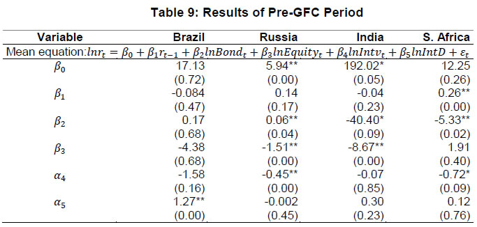 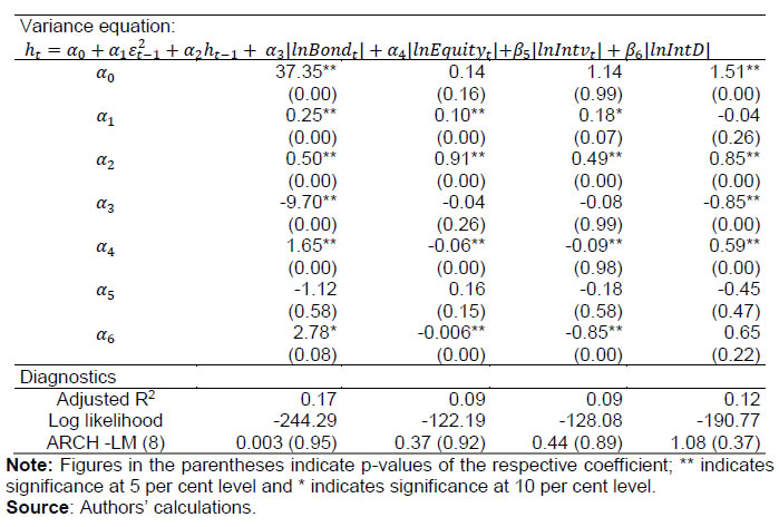 Table 9 displays the results of pre-GFC period equation. The overall bond and equity flows appreciate the currencies of Brazil, India and South Africa but depreciate the Russian Ruble. Intervention effectively reduces returns in Russia and South Africa while interest rate differential creates appreciation pressure on the Brazilian Real. In the variance equation, GARCH terms for all four countries are positive and statistically significant. The signs of coefficients of bond and equity flows are negative except for Brazil and South Africa, where the equity flows are positive showing that the equity flows increases volatility in their currencies. For the post-GFC period, the mean equation results re-confirm that bond and equity inflows create appreciation pressure on the BRICS currencies (Table 10). The intervention coefficient is negative in mean and variance equations implying that all the BRICS central banks have been able to successfully reduce the exchange rate returns as well as the volatility in the returns through foreign exchange market interventions. In the case of interest rate differential, we get mixed results. For India and South Africa, the negative sign indicates the interest rate differential appreciates their currencies. However, the positive coefficient shows that it depreciates Brazil Real. 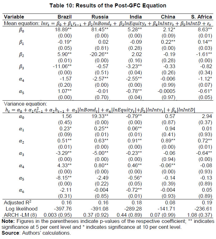 In the variance equation, the bond flows coefficients are negative and statistically significant indicating that the bond flows reduce volatility in the exchange rate returns, while equity flows increase volatility in Brazil, Russia and India. For China, we get a negative sign for the equity flow coefficient, although the coefficient size is small (0.06) indicating that the equity flows reduce volatility. For South Africa, the coefficient was not statistically significant. The intervention coefficient is negative for all the BRICS countries but is significant only for Brazil and India, indicating through interventions, these countries can reduce volatility in their returns. For the interest rate variable, we obtain mixed results. Exchange rate volatility adversely impacts market sentiments and thereby foreign trade and economic growth. Since BRICS represent an emerging economic block, foreign capital flows get easily attracted to these economies for higher returns. However, it has been observed that capital flows are often associated with exchange rate volatility. In this context, the paper finds that the foreign portfolio flows impact exchange rates and increase volatility in the foreign exchange market. While portfolio flows in both debt and equity segments create appreciation pressures on domestic currencies, the size of the coefficients differs across countries. Our findings differ from the results of some earlier studies that portfolio flows in equity market impact exchange rate volatility more than those in bond market (Siourounis, 2011). We observe that after the Global Financial Crisis, equity flows increased volatility in the exchange rate returns in BRICS currencies, while bond flows reduced it. While the interest rate differential has led to an appreciation in the Indian Rupee and South African Rand, it has resulted in a depreciation of the Brazilian Real. Our findings suggest that intervention by BRICS central banks have been useful in reducing volatility, though the effectiveness of such interventions varies from country to country. Central banks need to assess the impact of portfolio flows on their exchange rate markets. They also need to use a combination of various instruments based on their market analysis, which can address the undue volatility in their exchange rates. @ Dipak R. Chaudhari (dipakrchaudhari@rbi.org.in) and Prabhat Kumar are Assistant Advisers in Reserve Bank of India and Pushpa Trivedi is a Professor at Shiv Nadar University, Chennai. * The authors thank the anonymous referee and Amarendra Acharya for their useful comments on the paper during the DEPR Study Circle. We are grateful to the DRG team for their comments and feedback in revising the paper. The views expressed in the paper are those of the authors and not of the institutions to which they belong. 1 As per the IMF’s Balance of Payment Manual (6th edition), the FDI is the significant influence that gives the investor an effective voice in management (10 per cent or more of voting stock) while FPI is an investment where the owner holds less than 10 per cent of a company's shares (IMF, 2012). 2 The five countries of the “Fragile Five” include Brazil, India, Indonesia, South Africa and Turkey. References Altunöz, U. (2020). Determining the Interaction of the International Portfolio Flows with Exchange Rate Volatility in Developing Countries. World Journal of Applied Economics, 6(1), 41-54. Ananchotikul, N., & Zhang, L. (2014). Portfolio Flows, Global Risk Aversion and Asset Prices in Emerging Markets. IMF Working Papers, 14(156), 1. https://doi.org/10.5089/9781498340229.001 Aroul, R. R., & Swanson, P. E. (2018). Linkages Between the Foreign Exchange Markets of BRIC Countries—Brazil, Russia, India and China—and the USA. Journal of Emerging Market Finance, 17(3), 333–353. https://doi.org/10.1177/0972652718800081 Aydoğan, B., Vardar, G., & Yelkenci, T. (2020). Revisiting portfolio flows–exchange rate nexus in emerging markets: a Markov Regime Switching MGARCH approach. In Macroeconomics and Finance in Emerging Market Economies. https://doi.org/10.1080/17520843.2020.1814376 Baillie, R., & Bollerslev, T. (1989). The Message in Daily Exchnage Rates Condaitional-Varianve Tale. In Journal of Business and Economic Statistics (Vol. 7, Issue 3, pp. 297–305). Behera, P., & Mishra, B. R. (2020). Determinants of Bilateral FDI Positions: Empirical Insights from ECs Using Model Averaging Techniques. Emerging Markets Finance and Trade, 1–17. doi:10.1080/1540496x.2020.1837107 Caporale, G. M., Menla Ali, F., Spagnolo, F., & Spagnolo, N. (2017). International portfolio flows and exchange rate volatility in emerging Asian markets. Journal of International Money and Finance, 76, 1–15. https://doi.org/10.1016/j.jimonfin.2017.03.002 Chakraborty, I. (2006). Capital Inflows during the Post-Liberalisation Period. Economic and Political Weekly, 41(January 14), 143–150. Combes, J. L., Kinda, T., & Plane, P. (2012). Capital flows, exchange rate flexibility, and the real exchange rate. Journal of Macroeconomics, 34(4), 1034–1043. https://doi.org/10.1016/j.jmacro.2012.08.001 Dornbusch, R. (1980). Exchange Where Do Rate We Economics . Stand ? Brookings Papers On Economic Activity, 1980(1), 143–205. Dua, P., & Sen, P. (2013). Capital Flows and Exchange Rates: The Indian Experience. Indian Economic Review, 48(1), 189–220. https://econpapers.repec.org/RePEc:dse:indecr:0069 Ferreira Filipe, S. (2012a). Equity order flow and exchange rate dynamics. Journal of Empirical Finance, 19(3), 359–381. https://doi.org/10.1016/j.jempfin.2012.03.002 Ferreira Filipe, S. (2012b). Equity order flow and exchange rate dynamics. Journal of Empirical Finance, 19(3), 359–381. https://doi.org/10.1016/j.jempfin.2012.03.002 Frankel, J. (2007). On the Rand: Determinants of the South African Exchange Rate. South African Journal of Economics, 75(September), 425–441. Froot, K. A., O’Connell, P. G. J., & Seasholes, M. S. (2001). The portfolio flows of international investors. Journal of Financial Economics, 59(2), 151–193. https://doi.org/10.1016/S0304-405X(00)00084-2 Garcia, M. (2013). Should Brazil’s central bank be selling foreign reserves. URL: http://voxeu. org/article/should-brazil-s-central-bank-be-selling-foreign-reserves. Gautam, S., Chadha, V., & Malik, R. K. (2020). Inter-linkages between real exchange rate and capital flows in BRICS economies. Transnational Corporations Review, 12(3), 219–236. https://doi.org/10.1080/19186444.2020.1779525 Granger, C. W. (1988). Causality, cointegration, and control. Journal of Economic Dynamics and Control, 12(2-3), 551-559. Hau, H., & Rey, H. (2006). Exchange rates, equity prices, and capital flows. Review of Financial Studies, 19(1), 273–317. https://doi.org/10.1093/rfs/hhj008 Herrmann, S., & Mihaljek, D. (2013). The determinants of cross‐border bank flows to emerging markets: New empirical evidence on the spread of financial crises. Economics of Transition, 21(3), 479-508. Huang, A. Y., Peng, S. P., Li, F., & Ke, C. J. (2011). Volatility forecasting of exchange rate by quantile regression. International Review of Economics & Finance, 20(4), 591-606. IMF. (2012). Balance of Payments Manual, Sixth Edition. Balance of Payments Manual, Sixth Edition. https://doi.org/10.5089/9781589068179.069 In-Mee Baek. (2006). Portfolio investment flows to Asia and Latin America: Pull, push or market sentiment? Journal of Asian Economics, 17(2), 363–373. https://doi.org/10.1016/j.asieco.2006.02.007 Kanamori, T., & Zhao, Z. (2006). The Renminbi Exchange Rate Revaluation: Theory, Practice and Lessons from Japan. https://www.adb.org/sites/default/files/publication/159375/adbi-renminbi-exchange-rate.pdf Karakaplan, M.U., Kutlu, L. & Tsionas, M.G. A solution to log of dependent variables with negative observations. J Prod Anal 54, 107–119 (2020). https://doi.org/10.1007/s11123-020-00587-5 Kodongo, O., & Ojah, K. (2012). The dynamic relation between foreign exchange rates and international portfolio flows: Evidence from Africa's capital markets. International Review of Economics & Finance, 24, 71-87. Kohli, R. (2015). Capital Flows and Exchange Rate Volatility in I ndia: How Crucial Are Reserves?. Review of Development Economics, 19(3), 577-591. Mohanty, M. S., & Berger, B.-E. (2013). Central bank views on foreign exchange intervention. Journal of Economic Literature, 25(73), 55–74. Ndou, E., Gumata, N., & Tshuma, M. M. (2019). Exchange rate, second round effects and inflation processes: Evidence from South Africa. https://doi.org/10.1007/978-3-030-13932-2 Neely, C. J. (2008). Central bank authorities' beliefs about foreign exchange intervention. Journal of International money and Finance, 27(1), 1-25. Pattanaik, S. (2001). Exchange Rate Dynamics: An Indian Perspective. Reserve Bank of India Occasional Papers, 22(1, 2 and 3), 141–153. Rafi, O. P. C. M., & Ramachandran, M. (2018). Capital flows and exchange rate volatility: experience of emerging economies. Indian Economic Review, 53(1–2), 183–205. https://doi.org/10.1007/s41775-018-0031-1 Rashid, A., & Husain, F. (2018). Capital Inflows, Inflation, and the Exchange Rate Volatility : An Investigation for Linear and Nonlinear Causal Linkages. The Pakistan Development Review, 52(3), 183–206. Rafi, O. P. C., & Ramachandran, M. (2018). Capital flows and exchange rate volatility: experience of emerging economies. Indian Economic Review, 53(1), 183-205. Reserve Bank of India. (2021). Report on Trend and Progress of Banking in India: 2020–2021. Salisu, A. A., Cuñado, J., Isah, K., & Gupta, R. (2021). Stock markets and exchange rate behavior of the BRICS. Journal of Forecasting, 40(8), 1581–1595. https://doi.org/10.1002/for.2795 Shankar, Rashmi, Distinguishing between Observationally Equivalent Theories of Crises (2002). Available at SSRN: https://ssrn.com/abstract=636288 Shi, G., & Liu, X. (2020). Stock price fluctuation and the business cycle in the BRICS countries: A nonparametric quantiles causality approach. Finance Research Letters, 33(January 2019). https://doi.org/10.1016/j.frl.2019.06.021 Singh, B. (2012). Changing contours of capital flows to India. Economic and Political Weekly, 47(43), 58–66. Singh, D., Theivanayaki, M., & Ganeshwari, M. (2021). Examining Volatility Spillover Between Foreign Exchange Markets and Stock Markets of Countries such as BRICS Countries. Global Business Review. https://doi.org/10.1177/09721509211020543 Siourounis, G. (2011). Capital Flows and Exchange Rates: An Empirical Analysis. SSRN Electronic Journal, January 2003. https://doi.org/10.2139/ssrn.572025 Uctum, M., & Uctum, R. (2011). Crises, portfolio flows, and foreign direct investment: An application to Turkey. Economic Systems, 35(4), 462–480. https://doi.org/10.1016/j.ecosys.2010.10.005 Ul Sabeeh, N., & Mehmood, A. (2020). Collective Correlation Between Exchange Rate and Stock Prices: A Case of G20 Economies (2005 – 2019). SSRN Electronic Journal, 1–33. https://doi.org/10.2139/ssrn.3550900 Annex 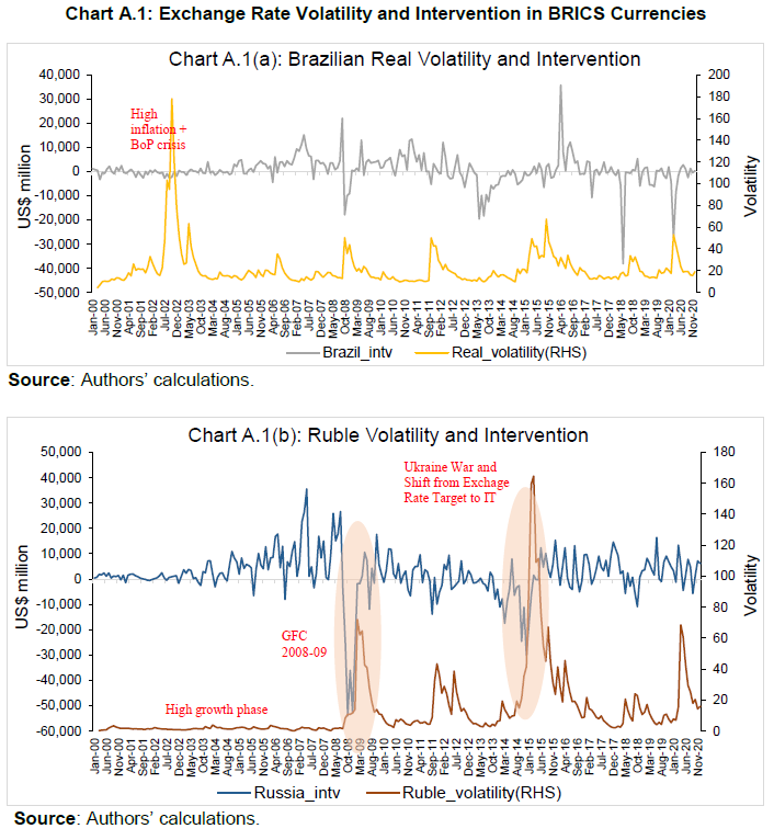 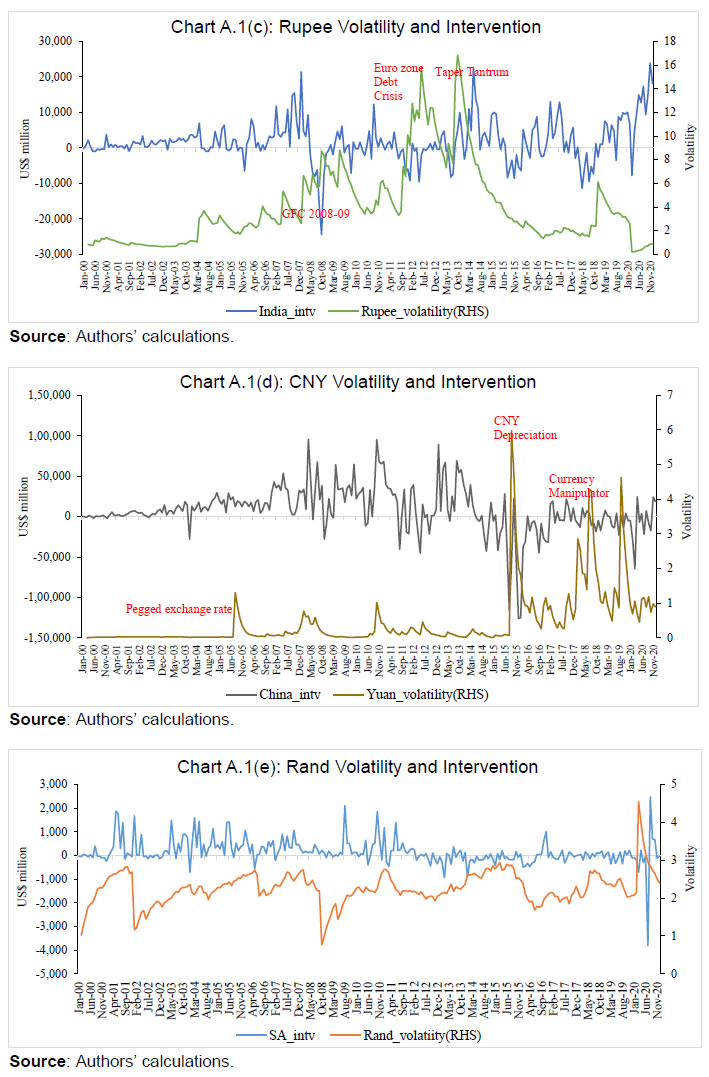 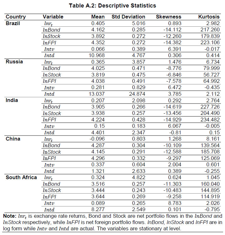 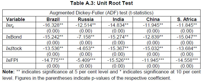
| ||||||||||||||||||||||||||||||||||||||||||||||||||||||||||||||||

हे पेज शेअर करा:


भारतीय रिझर्व्ह बँक मोबाईल ॲप्लिकेशन इंस्टॉल करा आणि नवीनतम बातम्यांचा त्वरित ॲक्सेस मिळवा!
आमचे अॅप इंस्टॉल करण्यासाठी QR कोड स्कॅन करा


पेज अंतिम अपडेट तारीख:


