 IST,
IST,
RBI WPS (DEPR) :22/2011: Credit and Growth Cycles in India: An Empirical Assessment of the Lead and Lag Behaviour
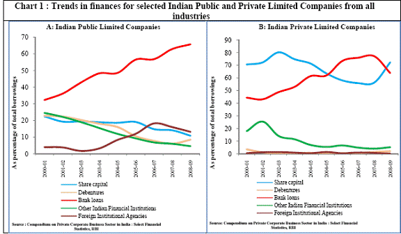
RBI Working Paper Series No. 22 Abstract * Procyclicality in the flow of credit has been a factor underpinning the magnified amplitudes of boom and bust phases of the business cycle, particularly in bank dominated financial systems. This paper studies the lead-lag pattern in the interaction between credit and growth cycles of India at three levels i.e. at the aggregate level for annual GDP growth, at the sectoral level across agriculture, industry and services, and also across major industries. The study focuses on three distinct periods, viz., 1950-51 to 1979-80, 1980-81 to 1990-91 and the post-1991 period and finds that there has been a significant transformation in the direction of credit-output causality during the period of analysis - from output being predominantly driven by credit in the pre-1980s period to nearly no relationship between the two during the 1980s and further to credit being primarily driven by output in the post-reforms period. For the non-agricultural sector as a whole, unidirectional causality from output to credit in the post-reforms period reiterates the importance of output in determining the quantum of flow of credit to non-agricultural sector in India. However, at the industry level, the study finds that a few industries exhibit bidirectional causality, indicating higher risks from procyclicality. Most strikingly, the study finds that the credit intensity of growth declines only in the second half of a contractionary phase of the business cycle, which generally continues in the first half of the expansionary phase of the business cycle. Similarly, the increase in credit intensity becomes more visible only in the second half of the expansionary phase, which persists in the first half of the contractionary phase of the business cycle. The study finds a lead role of credit for some industry groups which suggests that monetary and macro-prudential policies could at times operate through shifts in credit trends in managing inflation and promoting financial stability. However, in general, the absence of causality from credit to output growth in the post-reforms period emphasizes the need for more directed flow of and easy access to credit to all sectors for monetary policy to have the desired impact on output growth in the economy. JEL Classification: E3, E32, E51. Keywords: Procyclicality, Business Cycles, Growth Cycles, Credit Cycles. INTRODUCTION Cyclical patterns in aggregate economic activity and deviations from the equilibrium growth path have been observed ever since economic activities started to be measured. With the advent of macroeconomics and with an increasing use of fiscal and monetary policies for countercyclical stabilization, there has been a rise in the interest to understand the nature and causes of the recurrent fluctuations in output and growth. In the last two decades, the world has experienced quite a few economic crises in emerging economies as well as one major crisis in an advanced economy. In this context, one dimension of the policy debate has focused on leverage, the role of financial intermediation and credit market frictions in explaining economic instability, both during normal and crisis times. Credit has undoubtedly emerged as one of the most influential variables in the modern economy, despite increasing importance of other financial instruments in technologically advanced and interconnected financial markets. There is strong cross-country evidence that large imbalances in credit flows have been one of the most important causal factors behind the recurrent crises since the Great Depression of the 1930s. Besides, procyclicality of credit has been highlighted as a main cause in increasing the amplitudes of the output cycles, in effect exacerbating the economic cycles. To policymakers, cycles are of foremost significance since the positive and negative deviations from the trend growth path provide the trigger for policy actions. A Central Bank may want to forecast the extent of deviations in order to put in place appropriate policy measures, particularly when these fluctuations seem to originate from demand side imbalances. This is in sharp contrast to the real business cycle theory (Lucas, Prescottet al) which holds that business cycles are natural and efficient responses of the economy to changing production technology under the assumption of wage price flexibility. As such they advocate that the policymaker should not try to stabilize the economy since these fluctuations are optimal responses set into force by the ‘invisible hand’ in response to technology shocks. So far no view has actually won over the other and both views seem to have their own weights. Credit is considered one of the most relevant of all demand indicators for monetary policy in its role to stabilize demand. With monetary policy able to alter the path of credit growth directly, credit naturally emerges as a focal point of research on business cycles. This provides the basis for a study on the relationship between credit and growth, in lines of the lead-lag dynamics between business cycles and credit cycles. Against this background, this paper focuses on the “lead and lag relationship” between credit cycles and growth cycles for the Indian economy. Starting with the basic question, as to whether credit leads or lags behind growth in the economy as a whole and how the relationship varies from sector to sector, this paper examines the position at a micro level, from an industry point of view using Indian corporate sector data. Although there is no dearth of research on credit or business cycles, the dynamics of lead-lag relationship is a relatively new area where more research is required for a better understanding of credit as an indicator of business cycles, which will be helpful for formulating both monetary and macro-prudential policies. Section 2 explores the literature in this area, along with a brief description of the theories as well. In Section 3, trends in financing of Indian corporate firms and credit intensities in India are analysed. Section 4 presents the empirical analysis and inferences drawn from the analysis. Section 5 presents concluding observations, with an emphasis on policy implications from the empirical analysis. SECTION 2 Research on credit and growth interactions The role of credit in economic growth has been an area of extensive theoretical research. Schumpeter (1911) in his innovation theory talks about the essentiality of bank credit to introduce something entirely new for breaking the stationary equilibrium in which the society exists, which hints about the role played by credit in creating fluctuations. In a Schumpeterian world, bank credit increases money income, which in turn increases the demand for the products of the old industries in relation to supply. As profits increase, old industries expand by borrowing from banks. This induces a secondary wave of credit inflation. Over-optimism and speculation add further to the boom. After a period of gestation, new products start appearing in the market, displacing the old ones. As the demand for old products decrease, old firms contract output. As the innovators start paying out the bank loans out of profits, the quantity of money decreases and prices tend to fall. Profits decline. Depression ensues when uncertainty and risks increase, leading to credit deflation. The upswing is brought about once again by a new set of innovations and a new expansion in bank credit. Credit and growth, thus, exhibit bidirectional causality in Schumpeter’s theory. The linkage between lending policies of banks and credit cycles is an upcoming area of research, since it is believed that banks’ discretion is one of the foremost factors which influence credit. Variations in asset prices, which are offered as collaterals by the borrowers, change the lending policies undertaken by banks. Prices of assets are directly linked with the state of the economy and demand conditions. This collateral requirement amplifies business cycle fluctuations as observed by Kiyotaki and Moore (1997). They analyse the problem of contracts between borrowers and lenders, which always face a risk of default in an environment where value of a project cannot be known by the lender, as a result of which borrowing is tightly constrained by the value of collateral. During recessionary times, when price of capital falls, making it less valuable as collateral, firms have to reduce their borrowings and limit production, thereby worsening the recession. Credit restrictions can potentially amplify small shocks to the economy, giving rise to large output fluctuations and can be highly pro-cyclical. Minsky (1993), in his seminal paper called the ‘financial instability hypothesis’, provides further evidence to the proposition of procyclicality of credit by showing that over periods of prolonged prosperity, the economy transits from financial relations that make for a stable system (dominated by ‘hedge finance’ units) to financial relations that make for an unstable system (engaged in ‘speculative and Ponzi’[1] finance). If banks’ risk taking capacity varies regularly over time, the quantum of credit is bound to have ups and downs. Strategic interaction between banks leads to ‘herd behaviour’ amongst banks or bank behaviour might come to be dominated by the moves taken by a few large banks which accentuates the cycles. This brings to the forefront the issue of dependence of the real economy on financial stability. Rational banking would require banks to lend to borrowers with projects of positive net present value. Yet it has been the case that loans issued are correlated with changes in the condition of those demanding credit, irrespective of the prospects of the projects. Rajan (1994) shows that banks try to influence the perceptions of their equity-holders by manipulating their current earnings at the cost of dependability of their loan portfolios, which are not readily observable by the market. He shows that banks exacerbate demand expansions by funding negative NPV projects and accentuate contractions by not funding positive NPV projects. The prudential behaviour of banks has been extensively researched. The supply of credit can change with the attitude of banks towards risks over different phases of the business cycle. There are two kinds of risks to the health of the financial system. First, the actual/potential risk, which grows when the economy is expanding and banks become overly optimistic and reckless in issuing debt. The potential risk becomes the realized risk only after the boom peaks off and profits fall and loan repayments are defaulted upon. Kent and D’Arcy (2001) explain procyclicality on the basis of how some banks would act on the basis of actual risk (rather than realized risk) and would adopt procyclical prudential behaviour and some others will adopt countercyclical behaviour. He finds that the former tends to amplify the business cycles while the latter reduces it. Second, financial instability could also ensue from mis-measurement of these risks. According to Borio, Furfine and Lowe (2001), risks are underestimated in booms and overestimated in recessions due to short horizons in risk measurement methodologies and insufficient attention paid to correlations in default risks across borrowers and institutions. Banks fail to increase provisions in economic booms and constrain lending in recessions, contributing to the procyclicality in the financial system. In a 2004 study, Morgan and Lown found from a survey on opinion of loan officers of major US banks on the credit standards set by their banks that credit is correlated to the standards set by banks. Kiyotaki (1998) addresses the credit market frictions in terms of the question that in the exchange of present goods for future goods in a competitive general equilibrium framework, who will ensure that future goods are delivered to the agent who supplies present goods? In a decentralised economy, this very lack of guarantee creates the financial imbalances, which affect the real economy. Review of Methodologies Econometric methods to analyse the inter-relationship between any two variables generally range from vector auto-regression (VAR) to co-integration and Granger causality tests. However, lead-lag studies generally depend on peak-and-trough analysis, Granger causality tests and cross-correlations of which the latter two tests are more objective in nature. Lead-lag analysis is best done on the cyclical components extracted from the time series. There are various filters to extract the cycles as well as exponential smoothing methods. Samantaraya (2007) uses the Hodrick-Prescott (HP)-filter and the Band-Pass (BP) filter to extract the cycles in credit and GDP and found pronounced co-movement between the two for the post mid-1980s. Although Aburachis (2010) uses the co-integration test on quarterly US data over the period 1952-Q2 to 2007-Q2 (on total credit growth and the ratio of GDP growth to the output gap) to understand the long-run relationship, he relied on the Granger causality test to ascertain the lead-lag relationship on shorter periods based on business cycle turning points as designated by the National Bureau of Economic Research. His results point towards causality running from GDP/output gap to credit growth for 4 of the five turning points analysed. In a one of its kind study on the credit-growth nexus in the Indian context, Samantaraya (2007) studied the contribution of Basel prudential norms to the procyclicality of credit by using panel data techniques. He used real GDP growth and aggregate bank non-food credit in real terms (adjusted by implicit GDP deflator) since the 1950s and found a very high degree of correlation between these two. As a testimony to the above discussion on credit-GDP cyclical linkages and the role played by banks in it, the panel data model estimated by Samantaraya (2007), which used a total of 54 public/ private/ foreign banks over the period 1995-96 to 2007-08 (when the financial sector experienced greater market orientation), shows that economic growth, capital requirements and loan loss provisioning could significantly explain the procyclicality of bank credit in India since 1990s. There is a more than obvious linkage between credit cycles and business cycles. Procyclicality of credit has manifested with each and every economic crisis of the past century. If the state of the economy can be termed as ‘good’ and ‘bad’, good times provoke excessive and unscrutinized lending by banks and other non bank financial institutions due to expected high returns and low probability of default. This leads to over-heating of the economy during the expansionary phase of the economy. Prices rise without the equivalent increase in output. Loans are converted into bad loans. This means that a lot of the recipients of the loans may not be able to repay. As recession sets in, banks incur losses. A lot of bad debt makes them excessively cautious in terms of lending to save their eroding profits. Just when the economy would need credit badly, in order to boost itself out of the contractionary phase, banks would not be willing to lend since borrowers would not be able to put up sufficient collaterals because the values of collaterals would have declined in the recession. A common explanation for the procyclicality of the financial system is information asymmetries between lenders and borrowers. When economic conditions are depressed and collateral values are low, due to asymmetric information even borrowers with profitable projects may find it difficult to obtain funding. Borio, Furfine and Lowe, 2001 observed that ‘Periods of robust economic growth tend to be associated with significant increases in the ratio of credit to GDP, and recessions with declines in this ratio. Likewise, episodes of strong credit growth tend to go hand in hand with large increases in equity and property prices, and, to varying degrees, these prices tend to decline as credit contracts in the downswing.’ Morgan and Lown (2004), in similar lines, showed that in the US within the period 1967 and 2003 all but one recession were accompanied with slower credit growth. In his book “Money, Bank Credit and Economic Cycles”, Jesus Huerta De Soto also used the concept of artificial credit expansion without a parallel increase in voluntary household saving as a reason for growth bubbles and rise in price levels despite increase in productivity due to good technology shocks. Artificial increase in capital through newly-created loans does not bring in the practice of cautious investment to entrepreneurs. In the words of De Soto (2009), “Entrepreneurs act as if citizens had increased their saving, when they have not actually done so. Widespread dis-coordination in the economic system results: the financial bubble (“irrational exuberance”) exerts a harmful effect on the real economy, and sooner or later the process reverses in the form of an economic recession, which marks the beginning of the painful and necessary readjustment.” Estimation of cycles Business cycles are defined as recurrent sequences of alternating phases of expansion and contraction in the prime variables of the economy (like GDP or IIP), concurrent with a number of other real and financial variables in the economy so that all the variables are expected to move up and down more or less together, with leads and lags. Such ups and downs in the trend may come to persist for many years or only over one year. Economists define business cycles as a consensus of cycles. Moore (1982) observed that no single measure is either available for a long period or possesses all the desired attributes. This has given rise to the emergence of an area of research which studies the indicators of business cycles, a concept developed in the 1930s by the National Bureau of Economic Research. Indicators are primarily a pattern in the movement of time series which can be studied and put to use in triggering optimal policy actions. Leading, co-incident and lagging indicators are the three groups according to their reaching the cyclical turning points ahead of, at about the same time and after business cycle turning points, respectively. The stage of development in the indicators, whether it is preliminary, intermediate or final, say a lot about the initiation, continuance or reversal of policy measures. The same indicator may lead a cycle at some points of time and lag at other points of time or may be coincident with the cycle itself. The choice of indicator is based on both economic theory and empirical observation. The Organisation for Economic Cooperation and Development (OECD) compiles an index of leading indicators for all of its member countries excepting Iceland and the major six non-member economies (Brazil, China, India, Indonesia, Russian Federation and South Africa) which the Organization monitors. It uses variables on the basis of criteria like economic relevance, cyclical behaviour and data availability considerations for the composite leading indicator it calculates. In a paper titled “Composite Leading Indicators and Growth Cycles in Major OECD Non-Member Economies and Recently New OECD Member Countries”, the OECD mentions that in the case of India, the share of components related to monetary and financial statistics is over 55 per cent of the selected indicators which makes research on credit all the more necessary. In India, credit is an important source of information on business cycles since we have a quite dependable database. Cycle literature uses three kinds of definitions of cycles e.g. Business Cycles, Growth Cycles and Growth Rate Cycles. The first is the classical approach which defines them as recurrent phases of expansions and contractions in levels without any adjustments for long term trend. This approach dominated the studies of National Bureau of Economic Research. Graphically it would be the cycles in GDP or IIP plotted over time. The “classical” business cycles should have the expansion phase longer and larger than the contraction phase, but either phase must be persistent and pervasive enough to allow for significant cumulative and interactive effects and the sequence of up and down phases that constitutes the business cycle must be recurrent and not periodic (Zarnowitz and Ozylidirim, 2002). However, contractions in level GDP are not common with modern economies. This is true particularly for the emerging economies like India and China where GDP is growing continually and not coming down at any point of time. Although GDP can be growing continually, there are speed-ups and slowdowns in the rate of increase in GDP which give us the turning points. Many economic time series have experienced slowdowns in growth rates, which remain positive, but with no decline in levels. It has been the case also for countries like West Germany and Japan, which registered growth at very high rates in the post World-War II era of reconstruction. These economies experienced slowdowns in growth rather than absolute declines in overall economic activity. Frequently alternating periods of acceleration and slowdowns in growth rate during the decade of the 1960s raised questions about the practical use of classical business cycles in analysing cyclical movements in economic activities, leading to the emergence of the concept of growth cycles. Growth cycles, which are measured as fluctuations in the deviations of the principal indicators around their long-run trends, require trend estimation and elimination (Zarnowitz and Ozylidirim, 2002). The growth cycle is defined as deviations of the actual growth rate of the economy from the long-run trend growth rate. The high growth phase in a growth cycle coincides with the business cycle recovery and the expansion mid-way, while the low growth phase is identical to the later phase of expansion leading to recession. While the business cycle contractions include only the absolute decline in economic activity, growth cycle contractions, in addition, include slowdowns. The peaks in growth cycle approach tend to precede the business cycle peak (Mohanty, Singh and Jain, 2003). In this approach, the cyclical components in the chosen series are extracted using some time series method. The level series is assumed to be made up of a long term trend and short term cycles. There are several methods to extract cyclical components such as, Beveridge-Nelson (BN) decomposition, Unobserved Component method (UC) and Regime Shifting Decomposition. Sometimes models like structural VAR (SVAR) are used. Other methods include Hodrick-Prescott (HP) filter, Band Pass Filter and exponential smoothing. The third and more convenient approach is the ‘growth rate cycle’ approach which uses the fluctuations in growth rates to determine the business cycles. The growth rate cycles reflect the cyclical ups and downs in the growth rate of economic activity. In a business cycle recovery, till the peak of expansion growth rates shall be increasing, while the low growth phase is identical to the later phase of expansion leading to recession (Mohanty, Singh and Jain, 2003). While classical business cycles are longer in periods, the other two types of cycles are more numerous and generally shorter, and hence more in number. The business cycle analysis has been overshadowed by the latter two approaches mainly because economies have been showing a continuously growing trend in GDP in the later part of the twentieth century. In this paper, the latter two definitions of cycles have been used. More specifically, growth cycles have been used for the analysis at the macro and sectoral level and growth rate cycles have been used at the industry level[2].SECTION 3 Bank credit is still the most important source of finance for developing economies like India (Charts 1.A & 1.B). Fractional reserve banking, the brilliant innovation of modern banking, has made credit one of the most important financial variables of the economy. The linkages between credit and growth and the role of bank intermediation have left a question mark in the wake of the recent global crisis. The East Asian crisis (1997) showed how indiscrete lending by banks in good times could lead the economy to a bubble, a potential source of risk to the growth outlook. It is now more than evident that besides credit policies of the monetary authority, lending behaviour of banks can be a major determinant of credit flows. The evidence suggests that disruption of financial intermediation is a key feature of both recent and historical crises [Gertler and Kiyotaki (2009)]. In this section, we study the relative importance of the various sources of financing vis-a-vis bank credit for the Indian corporate sector.
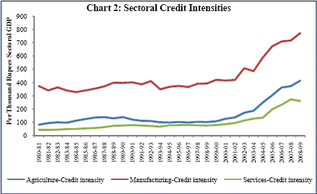
Chart 1.A shows that credit from banks is undoubtedly the most dominant source of finance for the public limited companies for the entire period (2000-01 to 2008-09). However, in the case of the private limited companies, share capital plays a predominant role in financing alongside bank credit (Chart 1.B). While the percentage of bank credit in total borrowings shows a continuous rising trend for the public limited companies, it has registered a major decline for the private limited companies around 2007-08. Chart 2 shows that credit intensity i.e. the amount of credit required per 1000 rupees of GDP is the largest for the manufacturing sector in India. It has also shown a steep rise since 2003-04. Credit intensity for the services sector has been consistently below the credit intensities of the other two sectors i.e. agriculture and manufacturing. This possibly signifies that the dependence on bank credit is lesser for firms in the services sector compared to the firms in the manufacturing sector where there exists a considerable lag between production and sales and hence, they depend more on credit.
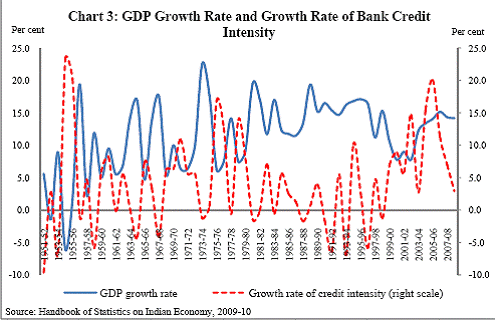
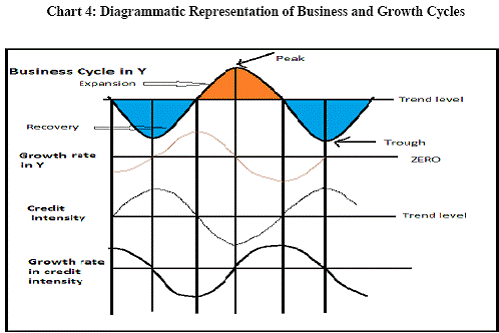
There are two types of sources of finances for production activities of firms, i.e. internal financing (corporate savings and retained profits) and external financing [debentures, bank loans, loans from domestic non-bank financial companies (NBFCs) and foreign institutional agencies]. In the external financing category, the first three are the domestic sources of finance while the last one is the foreign source. Table 1 provides information on the trends in internal sources of finances for Indian Public Limited Companies between 2001-02 and 2008-09. Tables 2 and 3 give a picture of how the various sources of external finance have evolved for Indian firms over the period 2000-01 to 2008-09. Non-availability of corporate sector data has constrained the information till 2008-09. Table 4 shows the relative position of bank credit compared to resources from domestic and foreign non-bank financial institutions over the period 2008-09 to 2010-11. The internal sources of funds as percentage of total sources of funds for public limited companies has almost halved between 2001-02 and 2008-09 for the manufacturing sector and this decline in the dependence on internal sources of funds is larger for services sector firms (Table 1). For the public limited companies under the manufacturing sector, bank loan has increased its share continuously, while the shares of debentures and credit from Indian NBFCs have shown decline over the period 2000-01 and 2008-09 (Table 2). For the public limited companies under the services sector, the picture is almost the same. Credit from foreign institutional agencies increased substantially during the period 2004-05 to 2006-07 for both manufacturing and services firms, but showed decline from 2007-08 to 2008-09 primarily reflecting the impact of the sub-prime crisis. Credit from Indian non-bank financial institutions declined substantially in 2005-06 for both sets of firms possibly due to changes in regulatory guidelines (RBI Annual Report 2003-04: the interest rates NBFCs could offer on public deposits and NRI deposits on a repatriable basis were reduced and aligned with those of banks). Bank credit, as a percentage of total borrowings, for the sample of public limited companies under manufacturing sector, stood at 70.7 per cent in 2008-09 - a little higher than 66.9 per cent for the sample under services sector (Table 2). Table 3 shows that for the private limited companies in India, bank credit has emerged the most important source of finance vis-à-vis other sources. However, bank credit to the private limited companies in the services sector has risen by lesser amount between 2000-01 and 2008-09 compared to the manufacturing sector firms. Relative to public limited companies, borrowings from foreign institutional agencies are very low for these firms. Table 4 shows that there has been a rise in bank credit flowing to the commercial sector in 2010-11 compared to 2009-10. Domestic non-bank resources have registered a significant decline in 2010-11 from 2009-10 possibly due to the restricted flow of credit to NBFCs from domestic banks due to the post-crisis liquidity crunch as well as tightening of prudential norms for NBFCs in the light of the systematic importance such institutions can assume. Foreign non bank resources show a continuous decline 2008-09 onwards possibly as an impact of the sub-prime crisis. Data from the Indian corporate sector summarily shows that domestic bank credit has emerged to be a dominant source of finance which is the core limiting factor for most businesses and therefore is expected to have a major impact on growth of the Indian economy. SECTION 4 Aggregate credit and growth cycles in India As discussed earlier, the main aim of this study is to understand lead-lag relationship between credit and economic growth in India through the use of growth cycles and growth rate cycles in credit and GDP. Bank credit, in India, is composed of food credit and non-food credit. However, food credit that is used for procurement of food grains is likely to be determined by external factors like monsoons as well as size of the marketed surplus and Government procurements. Hence, non-food credit has been used as the measure of credit. Bank credit in money terms is a nominal variable and its value is often related to nominal GDP. Given the emphasis of the paper on business cycles, Gross Domestic Product at factor cost at current prices was used to determine cycles. GDP is the most preferred choice especially to investigate cycles at quarterly or annual frequencies. In India, GDP data are available only at an annual frequency for a longer time period. Given the objective of the paper to study the evolution of cyclical patterns over time with changing structure of the economy, annual GDP and credit figures have been preferred. Accordingly, annual data from 1950-51 to 2010-11 were used. Credit intensity as a ratio of bank credit (C) to GDP (Y) gives an insight into how credit is moving over time with respect to movements in GDP. Chart 3 depicts growth rate in GDP at factor cost at current prices (Base year: 1999-2000) and growth rate in credit intensity[3] in India for the post- independence period. Growth in credit intensity reaches peaks when GDP growth rate reaches troughs. The co-movement in these two variables is better explained through Chart 4.
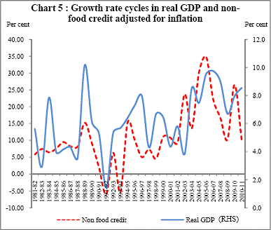
In a contractionary phase of a business cycle, the economy reaches a trough before recovering towards the trend level. Similarly, in an expansionary phase, the economy reaches a peak before it starts to cool down to the normal trend. In the recovery for the economy to pull up to the trend level, GDP shall increase at an increasing rate i.e. dY/dt > 0 and d2Y/dt2 > 0. Growth rate is nothing but ((dY/dt)/Y). What happens to the growth rate? Suppose GDP rises from Y1 to Y2 = 2 Y1 in period 1 and then from Y2 to Y3 = 4 Y2 (a simple illustration of GDP increasing at an increasing rate). Then when GDP rises from Y1 to Y2, growth rate is 1 but when the economy rises from Y2 to Y3, the growth rate is (Y3-Y2)/Y2 = (4Y2- 2Y1)/2Y1 = (8Y1-2Y1)/2Y1 = 3. So recovery in level GDP is coincident with the first half of expansionary phase in growth rate cycle (Chart 4). After reaching the trend level GDP, the economy still grows but GDP will now increase at a decreasing rate until level GDP reaches a peak. Growth rate falls but remains positive. This coincides with the second half of the expansionary phase of growth rate cycle. So, the first half of expansion in GDP is coincident with second half of the expansion in growth rate. At the peak level of GDP, growth rate is zero. Beyond the peak, the GDP starts falling and growth rate is negative and falling until it reaches a lower bottom where it starts rising again but is still negative. Growth rate reaches zero when the economy reaches another trough beyond which growth rate embarks upon another expansionary phase. If we map this cyclical pattern in GDP and its growth rate into growth rate in credit intensity and credit intensity in levels, what we see in India’s case is that credit intensity is decreasing during the latter half of contraction phase or recovery and it decreases further in the first half of the expansionary phase also. But it starts increasing in the latter half of the expansionary phase and increases till the economy reaches the trough. It is an illustration of the procyclicality of credit. As the economy starts overheating, credit per thousand rupees GDP (credit intensity) starts increasing. But as the economy tries to pull out of recession, credit per thousand rupees GDP falls aggravating the recession[4].[ What we observe in this case is that in the recovery phase of recession, credit intensity falls. It falls further in the first half of the expansionary phase till credit intensity reaches a trough. So increases in credit are lower than GDP increase in these two phases. From the second half of the expansionary phase onwards, credit intensity starts to rise till the economy reaches the trough of the business cycle. It implies that when both GDP and credit are declining, credit is declining at a lower rate than GDP. In such a scenario the credit intensity will actually increase instead of declining despite the decline in both the variables. Alternatively, we might look at the growth rate cycles in real GDP and in credit adjusted for inflation to see if a similar trend can be observed here. Chart 5 shows that the pattern observed with credit intensity growth and GDP growth (Chart 3) is also observed with credit and GDP growth in real terms but is seen clearly only after 1992-93. In the recovery phase of GDP cycle (first half of expansionary phase of growth rate cycle, refer to Chart 4), credit starts declining until it reaches a trough which coincides with the economy reaching the peak in terms of GDP. Subsequently, when the GDP starts falling (first half of the contractionary phase in growth rate cycle), credit starts increasing until it reaches a peak, which coincides with GDP reaching a trough.
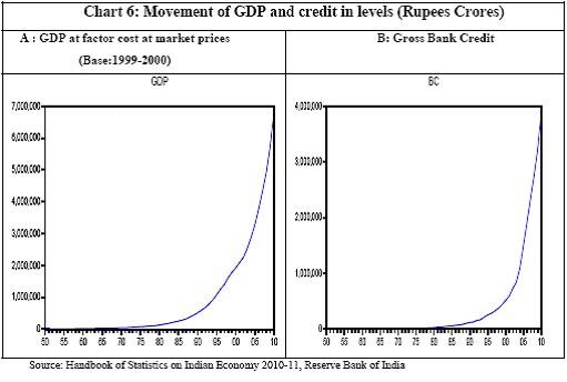
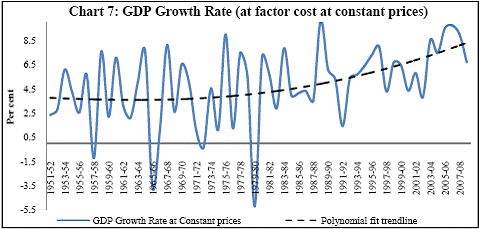
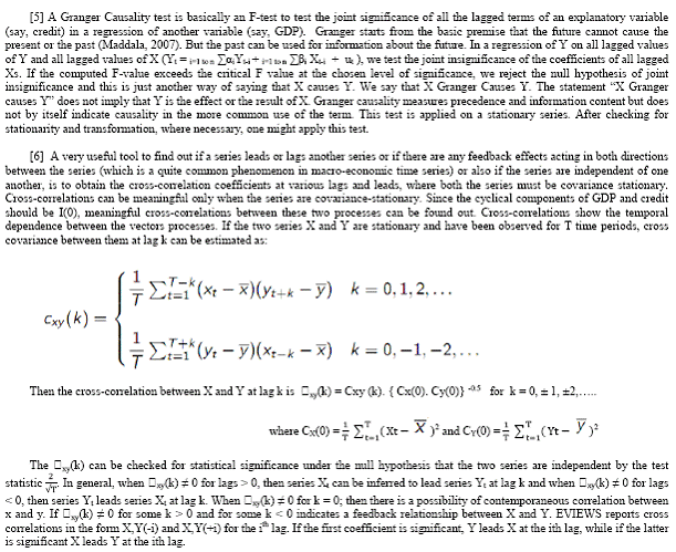
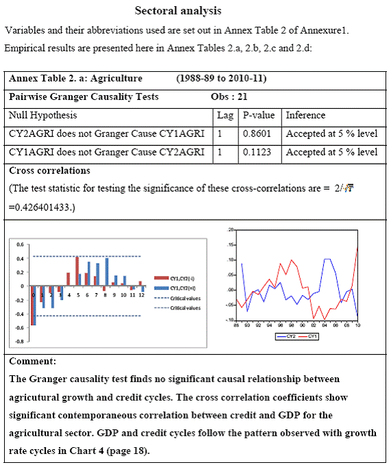
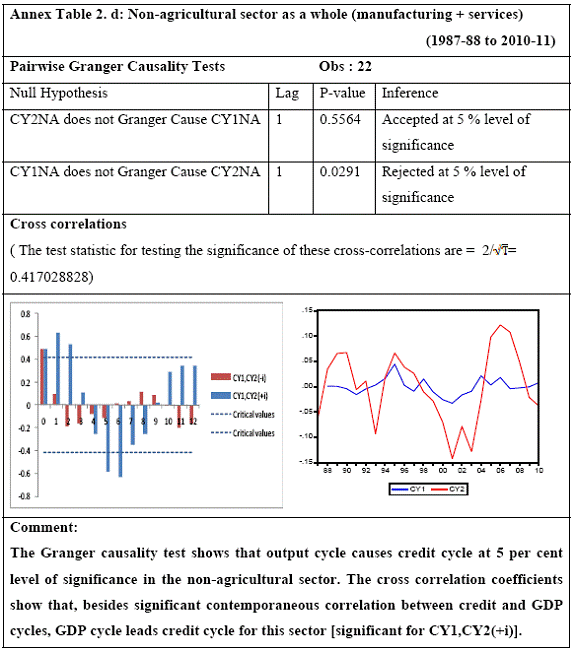
Granger Causality Test and Cross correlation coefficients Granger causality tests[5] and cross correlation coefficients[6] represent the methodology used to see whether credit leads or lags growth. These tests are done on growth/growth rate cycles to understand the direction of causality which has been tested for different time periods, different sectors of economic activity and for different industries[7]. Going beyond the classical business cycle consensus (the traditional NBER approach) that it is impossible to separate cycles from trend, the proponents of growth cycles believe that any annual macroeconomic series is composed of three components: trend, cycle and a random term. While the trend component shows the permanent growth in the series due to structural factors like technological change and improvement in total resources in the economy, the cyclical component shows ups and downs in the economy due to temporary factors like demand side imbalances and it may give us a better picture of the lead-lag relationship between credit and growth. Extracting a cycle involves identifying a series as I (1) i.e. with a unit root. If Yt ~ I (1) then it is possible to decompose Yt into a non stationary deterministic / stochastic trend component Pt and a stationary [I(0)] cyclical component Ct , such that Yt = Pt + Ct . Here, stochastic trend Pt captures shocks that have permanent effects on the level of GDP and the stationary component Ct represents the temporary effects of shocks. For the extraction of cycles the Hodrick – Prescott Filter[8] method was used. Further, both Granger causality tests and cross correlations analysis need the series to be stationary. This is to avoid the folly of non-sense or spurious regression first discovered by Yule who showed that spurious correlation could exist in non-stationary time series even if the sample is very large. So the extracted cyclical series being stationary time series can be used in our analysis. To determine the stationarity of the series Augmented Dickey Fuller test (ADF) and the Phillips-Perron (PP) tests were used[9]. To bring a uniformity in the stationarity of all the series used for causality analysis, only intercept was included in the test equations of the unit root tests, in effect testing whether the series is difference-stationary or not. An important practical question is the number of lagged terms to be used in the causality tests. The direction of causality critically depends on the number of lagged terms included. Sometimes it is possible for causalities to be significant for higher lags even though the underlying regression model is unstable. To solve the lag issue, underlying VARs are estimated[10]. It is considered that lag is optimum at which the Schwartz Information Criterion takes the minimum value and the VAR is stable as well, i.e. all roots of the VAR are less than 1. However, one must note that since there has been a change in the structure of the Indian economy over the 60 years of post independent economic history, structural breaks in dataset can give rise to anomalies in results. Over the span of 59 years, the country has undergone policy shifts and hence, experienced major changes in developmental strategies. This necessitates the unit root test results be validated by incorporating a structural break factor in the test, for example the Phillips-Perron unit root test would help in such a case. One can also see the structural breaks in the data by visual inspection. The structural breaks for Indian macroeconomic series can be easily seen in the non-linear movement of GDP and credit. GDP shows a sudden steep rise roughly from 1980 onwards, which is also the case for bank credit (Charts 6.A and 6.B). There is another major change in slope of the GDP curve roughly near 1990. In Chart 7, one could see that the polynomial trend of growth rate in GDP (Base: 1999-2000) changes to a steeper slope from 1979-80 onwards.
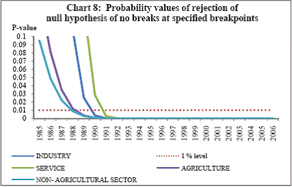
Research on India’s growth rate has divided the Indian growth story into three sub-periods: one from 1950-51 to 1979-80, another from 1980-81 to 1990-91 and third, from 1991-92 to 2010-11. India’s growth rate averaged the so called ‘Hindu’ rate of growth of 3-4 per cent for the first three decades after independence. The economy was, in general, believed to have undergone a huge structural change with the economic reforms of 1991 that ushered in a phase of globalisation and financial liberalisation in India. However, the actual process had started with the start of the 1980s when there was a considerable shift in the Government’s policies towards the private corporate sector, favouring privatization. While attempting to identify the structural breaks in India’s post-independence growth, Balakrishnan & Parameswaran (2007) used the Bai & Perron method to derive the break dates endogenously from the data set itself rather than pre-identifying and testing for statistical significance. They reported two break points (1980-81 and 1991-92) in the post-independence growth history of India thereby identifying three growth phases, pre 1979, 1980-1990 and post 1991 which have been used in this study. Charts 6.A and 6.B of the Gross Domestic Product at factor cost at market prices (Base: 1999-2000) and Gross Bank credit respectively show similarity in the temporal structure of the data. Both the series are non stationary. The structure of the data suggests the need for log transformation of both the series. Empirical Results The first part of the empirical analysis contains the analysis at a broader macro level from two perspectives: first, it is done over three sub-periods so that structural change in the economy is incorporated and second, it is done at a sectoral level for the post reform period. At a country-level, 59 data points are divided into three sub-periods: (1) 1950-51 to 1979-80, (2) 1980-81 to 1990-91 and (3) 1991-92 to 2010-11. Sectoral data on gross non-food bank credit in India is available from only 1980-81 at annual frequency. So the sectoral analysis is done for the post-reform period from the year where the structural break has been found to be significant by Chow test. A major drawback of the Chow test is that in a short time series it might report significant breaks for several points. Thus, in order to find the dates more specifically, Chow breakpoint test has been applied to various years to arrive at a single date where the break is most significant. After plotting the P-values for various years, that year is taken as a breakpoint where it goes below the critical 1 per cent level of significance (Chart 8). Accordingly, 1988-89, 1989-90, 1990-91 and 1987-88 are chosen as breakpoints for Agriculture, Manufacturing, Services and Non-agricultural sectors, respectively, and sectoral data have been analysed starting from these years till 2010-11.
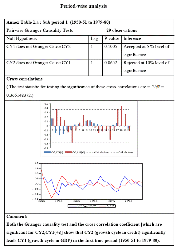
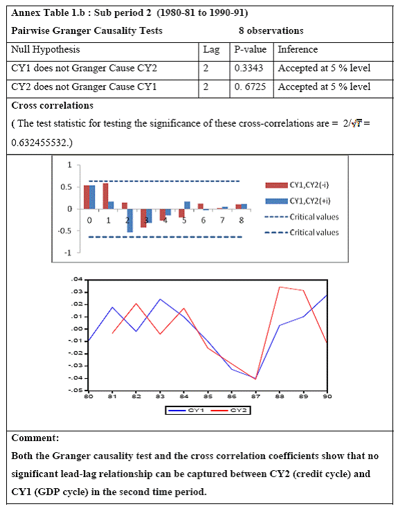
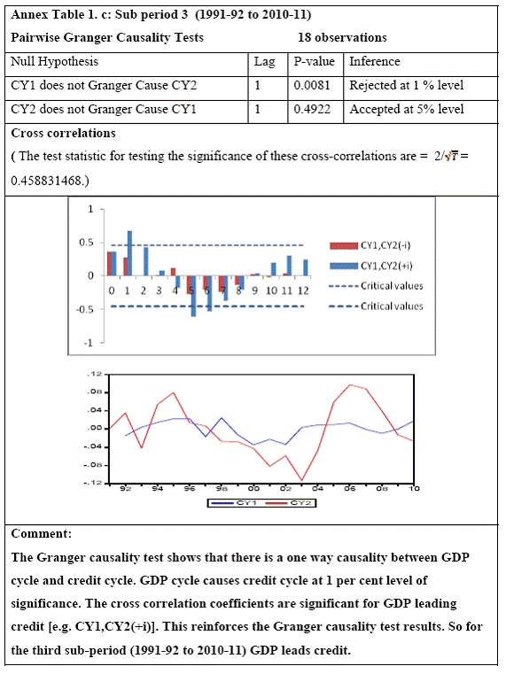
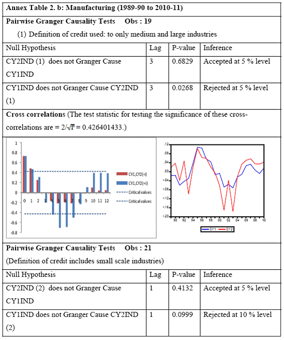
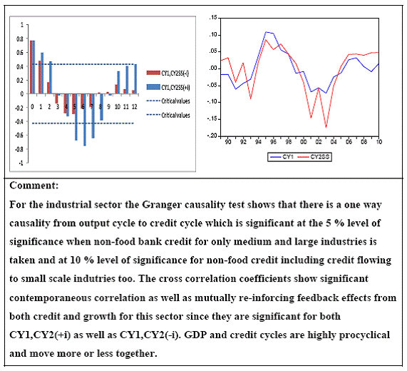
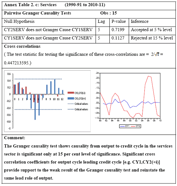
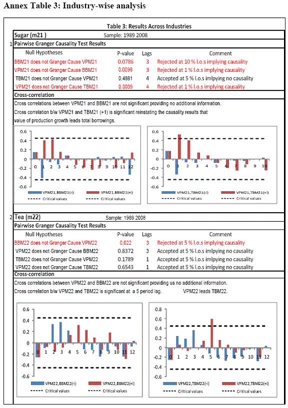
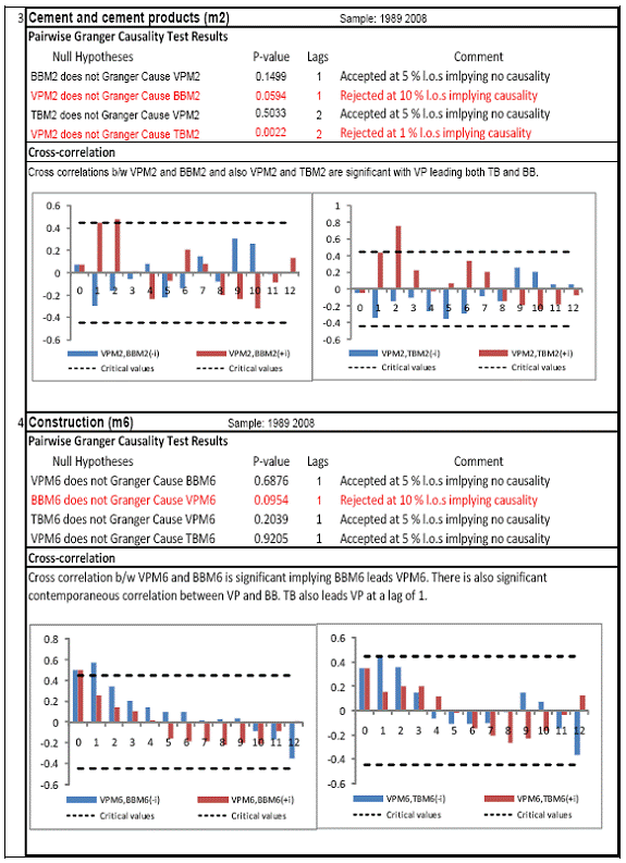
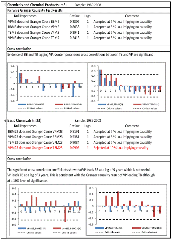
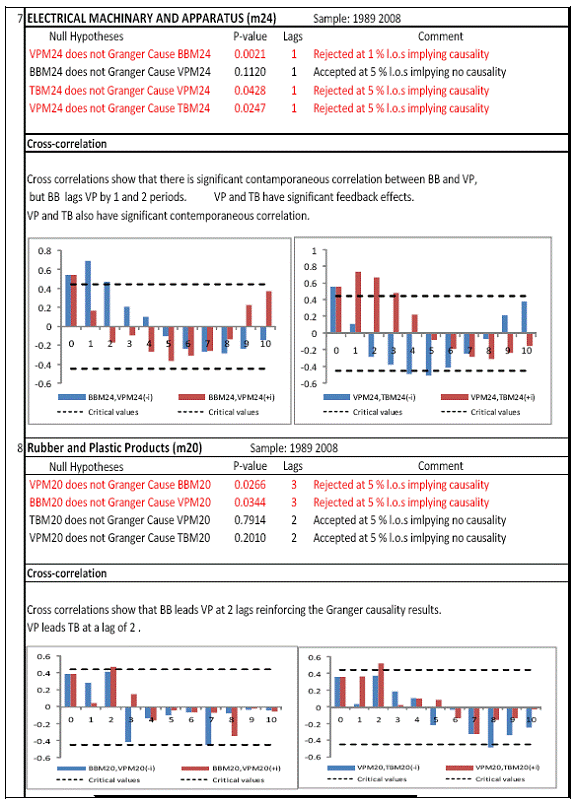
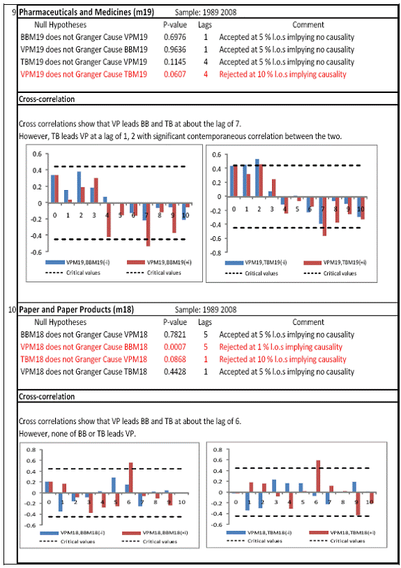
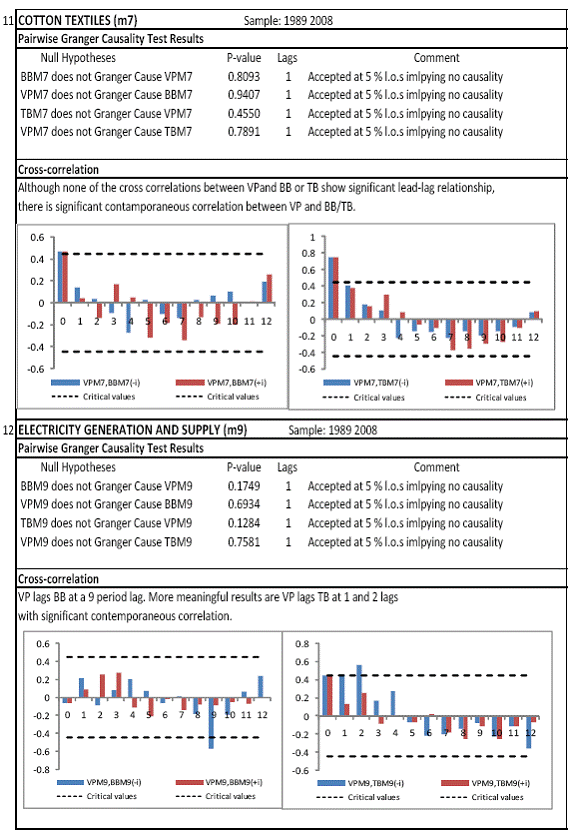
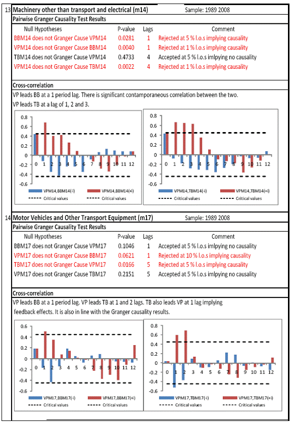
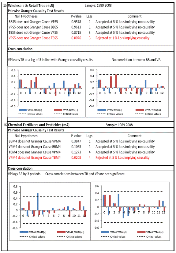
All macro level data have been taken from the Real-Time Handbook of Statistics on the Indian Economy (HBS) of Reserve Bank of India. To test for lead-lag relationship, growth cycles extracted by HP filter from log transformations of bank credit and gross domestic product data were used. Logarithm of GDP and logarithm of BC must necessarily be I (1) series for extracting the cyclical component. Non- stationarity in level but stationarity in the first difference is sufficient to show that a series is I(1). This is tested using the Augmented Dickey Fuller and Phillip Perron tests. The Hodrick Prescott filter is used on these I(1) series to extract the series of cyclical components which are again tested for stationarity. Only intercept is included in the test equations of all the ADF and PP tests to see if all the series are difference stationary. Results of these unit root tests are presented in Annexure 1. Detailed empirical results on Granger causality tests and cross correlations are presented in Annexure 2. Table 5 summarizes the major results, sub-period wise and sector wise. Industry-wise Analysis The second part of the empirical analysis is the industry-wise analysis. Following the analysis at sectoral level, an industry-wise analysis could provide a further perspective on the procyclicality of credit from a micro level in the Indian corporate sector. Data used for this study have been taken from the “Compendium on Private Corporate Business Sector in India: Select Financial Statistics (1950-51 to 2008-09)” brought out by Reserve bank of India. For the industry level analysis, bank borrowing figures under non-food credit have been used. The industry level analysis is conducted on growth rate cycles, i.e. growth rates in Value of Production (which alternatively combines Sales and Net change in Inventories) and gives a better picture of the real output of firms. Growth rates in Value of Production, Total Liabilities and Bank Borrowings of select Public Non-Government Non-Financial Companies for the period 1989-90 to 2008-09 have been used (mainly because of availability of data for that period only). One problem with this data set is that there are some years where two different overlapping sets of firms have been considered to arrive at two growth rate figures for the same year. In such cases, the figure pertaining to the set with the larger number of firms has been used. Various industries under manufacturing and services sectors have been assigned codes for simplicity of analysis (Table 6). The years for which data have been analysed are also given. Some of the industries could not be analysed statistically due to non-availability of data for enough number of periods to establish the stationarity of the series. Overall 16 industries have been analysed. For each industry, three variables have been used in the analysis which are Value of production (VP), Total borrowings (TB) and Bank borrowings (BB). Annual growth rates in these variables have been used. Major results for each industry are tabulated in Table 7. The industry –wise analysis has been summarized in Table 8. Detailed results and charts are presented in Annex Table 3 of Annexure 2. Interpretation of major findings This paper studies the lead-lag relationship between credit and growth in a step-wise fashion. First, it covers three sub –periods in post independent history of India, accommodating structural change in the economy; second, for the three sectors, i.e. agriculture, manufacturing and services; third, across individual industries. Financing of firms’ activities is one of the most important sources of information which is why this paper analyses data from the Indian corporate sector to get a clear picture of the risks in the economy in terms of procyclicality of credit and over dependency on credit. Firms are bulk borrowers. Several studies use data of borrowings by firms to understand credit growth. Period wise analysis shows an interesting change in the direction of output-credit causal relationship over the last six decades. In the period 1950-51 to 1979-80, there was a significant one way causality from credit cycle to growth cycle. During this period, India was a planned economy following the path of import substituting industrialization and credit can be seen to have significantly impacted growth. But the second period, 1980-81 to 1990-91, showed no significant causality between credit and growth as well as no significant cross correlations. The third sub-period, 1991-92 to 2010-11, shows causality from output to credit cycles significant at 1 per cent level. So it can be inferred that the direction of causality has changed over time from credit leading output to output leading credit. However, bidirectional causality between credit and output is still not evident in the Indian economy, although risks of procyclicality of credit can be seen in the second sub-period with more interconnectedness of financial institutions and the real and financial sectors under the liberalised regime in India. Indian manufacturing and services sectors, taken together as the non - agricultural sector, exhibit a one way causality from GDP cycle to non-food bank credit cycle. Also, the causality is significant at 5 per cent level. Cross correlations between credit cycle and output cycle reinforced the finding that GDP cycle leads credit cycle, with significant contemporaneous correlation between output and credit in their cycles. For the manufacturing sector, when credit only to medium and large industries is used to extract the credit cycle, the output to credit causality is significant at 5 per cent level. However, with inclusion of non food gross bank credit going to small scale industries, the output to credit causality is significant only at 10 percent level. This suggests that credit to small scale industries might be less procyclical in nature compared to credit to medium and large industries. However, along with significant contemporaneous correlation between credit cycle and growth cycle in the manufacturing sector, cross correlation coefficients are significant for both credit cycle leading output cycle as well as for output cycle leading credit cycle. Granger causality test indicates that the credit to output causality is insignificant for this sector. Nevertheless, the significant cross-correlations might indicate greater risks of procyclicality for the manufacturing sector in comparison to the services sector. The statistical evidence of GDP cycle Granger causing credit cycle in the services sector is weak. However, significant cross correlations between GDP cycle and lagged credit cycle provide support to the causality and it might be considered to be significant at 15 per cent level. When the agricultural sector was analysed exclusively, it was seen that output cycle Granger caused credit cycle at 15 per cent level of significance with no significant cross correlations in support of the test result. Nevertheless, this finding is on the expected lines of the dependence of agricultural output on various factors like monsoon conditions and minimum support prices. Possibly, expectations of farmers regarding output and the consequent credit demand emerging out of it is reflected in output causing credit. Sixteen industries were analysed statistically using the Granger causality test and the cross correlation test for second checking. Growth rate cycle was used for three variables: value of production, bank borrowings and total borrowings to find out the lead-lag relationship between credit and growth. Total borrowings were included in the study to accommodate for the possible impact of non banking sources of financing. The analysis shows that out of the 16 industries where data is available from 1989-90 to 2008-09, four of the industries show a two way causality implying higher risks from procyclicality of credit. These are: Electrical Machinery and Apparatus, Rubber and Plastic Products, Machinery other than transport and electrical, Motor Vehicles and Other Transport Equipment. These are the industries which can pose risks to the economy by amplifying the output cycles. Also the results for Electrical Machinery and Apparatus and Motor Vehicles and Other Transport Equipment are supported by the cross-correlation coefficients calculated for them. All the four industries play crucial roles in the economy and hence require strict monitoring of developments in credit-growth dynamics so that any imbalances can be corrected immediately. Another nine industries show one-way causality. These are: Tea, Sugar, Cement and Cement Products, Construction, Basic Chemicals, Pharmaceuticals and Medicines, Paper and Paper Products, Wholesale & Retail Trade and Chemical Fertilisers and Pesticides. The results for Chemical Fertilizers and Pesticides and Tea are not supported by the cross-correlation coefficients. Out of these, Sugar, Cement and Cement products and Basic Chemicals show value of production growth Granger causing both bank and total borrowings growth. In Paper and Paper products growth in value of production causes growth in bank borrowing only. This possibly shows that this industry depends mainly on domestic bank credit. Value of production growth impacts total borrowing growth only in the case of Pharmaceuticals and Medicines, Chemical Fertilisers and Pesticides and Wholesale & Retail Trade implying these industries are more likely to borrow from other sources of financing than domestic bank credit. Tea and Construction are industries where growth rate in bank borrowing leads to growth rate in value of production. Granger causality test result is supported by cross-correlations only for the construction sector. Credit can be inferred to be a strong determinant of output in the construction sector which points to the growing dependence of real sector output on credit in the Indian economy. In that respect this is a sector that needs constant monitoring to prevent the build-up of asset bubbles. However, there are no such industries where total borrowings, which include both domestic (bank and non-bank) and non domestic sources of finances, single-handedly impacts growth in output.This implies that Indian corporate sector is still more dependent on domestic bank credit rather than other sources. There are three industries - Cotton textiles, Chemicals and Chemical Products and Electricity Generation and Supply which show no significant causality between production growth and borrowings growth. Chances of procyclicality are least for these industries. However, significant contemporaneous correlations between growth in value of production and borrowings are seen in all three industries. For a bank dominated financial system, credit is the single-most important factor in the analysis of growth cycles. However, apart from boosting growth, credit can also be the factor that alone can cause sharp contraction in output and employment through credit squeeze. Understanding the nature of credit flows in the economy is one of the essential requirements for designing monetary and macro-prudential policies. The perception of banks towards the existing risks in the financial system leads to undesirable ups and downs in credit flows, which closely follow the business cycles. Research shows that the quantum of credit increases when the economy is booming and decreases when the economy goes into a recession because banks tend to loosen their credit standards in good times and tighten them in bad times. Moreover, output growth leads to credit growth, which in turn allows even higher output growth. If capacity addition lags behind credit induced growth in demand, over- heating and asset bubble risks increase. The procyclicality of credit magnifies the amplitudes of booms and busts within the cycles. One of the most vigorously debated issues in this context has been whether credit can be a leading or lagging indicator of growth and does the lead-lag relationship change over time. Another question that arises as a natural follow-on of the debate is that if credit is procyclical, to what extent it is so and in which segments of the economy. The findings of the paper, similar to findings of studies in context of other countries, suggest that the behaviour of credit in India vis-à-vis growth changes over different phases of the business cycle. The expansionary and contractionary phases of GDP consist of two distinct sub-phases. Credit intensity starts to fall in the second half of the contractionary phase and this decrease continues in the first half of the expansionary phase when the economy, just out of recession, tries to pick up on growth. In the early phase of the recovery, thus, credit growth may remain dampened. During the first half of the expansionary phase, credit intensity in fact dips below the trend. Credit intensity picks up in the second half of the expansionary phase. This is when credit intensity overshoots the trend level. This implies that in the first half of the expansionary phase credit lags behind growth, but it moves ahead of growth from the second half of the expansionary phase giving rise to plausible risks of overheating. The empirical findings point to transformation of “credit to growth” causality in the pre-1980s into “output to credit” causality post 1990s. The “output to credit” causality indicates procyclicality of credit. However, the absence of bi-directional causality between credit and output cycle in the Indian economy signifies the importance and success of macro-prudential measures. It was seen that when credit to small scale industries (that comes under priority sector lending) is included in the gross non-food bank credit to industries, it could reduce the significance of the output to credit causality. The study found by analysing sector-wise and industry-wise credit and output cycles that the lead behaviour of output is evident across the industrial sector which provides a case for considerable demand side pressures in the Indian economy. In general, the absence of causality from credit to output growth in the post-reforms period emphasizes the need for more directed flow of and easy access to credit in all sectors for monetary policy to have the desired impact on output growth in the economy. Non-agricultural sector, as a whole, shows statistically significant output to credit causality. At the industry level, higher procyclicality risks between credit and production could be identified for four industry groups like Electrical Machinery and Apparatus, Rubber and Plastic Products, Machinery other than transport and electrical, Motor Vehicles and Other Transport Equipment. Procyclicality risks were seen to be highest for ‘Electrical Machinery and Apparatus’ and ‘Motor Vehicles and Other Transport Equipment’. Credit is one variable that central banks could control and regulate in their attempts to avoid risks to inflation and financial stability objectives from overheating, credit-led asset price bubbles, and sudden pressure on NPAs during slowdown in economic activities. Unlike monetary policy, macro-prudential policies could be sector-specific, depending on the assessment of financial stability risks from specific sectors.The study looked into industry-wise credit-growth dynamics, and found that some industries are pro-cyclical, and also among them only a few industries being more procyclical than others. The study accordingly brings to the fore the question as to whether banks, whose lending portfolios are more exposed to industries with higher risks of procyclicality, should be more closely monitored. Further research on this is required, not only to provide support to a case for use of industry-wise prudential regulations but also to assess the role of credit in growth by measuring the productivity of a unit of credit in various industries. The lead role of credit over certain phases of the business cycle and for some of the industry groups suggests that monetary and macro-prudential policies could be aligned accordingly to enhance the effectiveness of managing inflation and financial stability implications of business cycles. @ Krittika Banerjee (krittikabanerjee@rbi.org.in) is Research Officer in the Department of Economic and Policy Research (DEPR), Reserve Bank of India. * The author is grateful to Shri Sitikantha Pattanaik, Director, DEPR for his valuable guidance on both theoretical and technical aspects that formed the basis of this paper and his constant encouragement. The author is thankful to Shri B. M. Misra, Officer-in Charge, DEPR for his useful suggestions that helped in strengthening the paper. She also very gratefully acknowledges the discussions with Shri Anand Prakash, Assistant Advisor and with Shri G.V. Nadhanael, Research officer, DEPR. Views expressed in the study are personal. [1] Borrowing units have been classified by Minsky (1993) into hedge finance units (which can fulfill all of their contractual payment obligations by their cash flows), speculative units (have to issue new equity to repay debt) and Ponzi units (the cash flows from operations are not sufficient, they have to borrow or sell to repay debt). [2] The choice of two different types of cycles is primarily due to the non-availability of enough data points for some industries at the industry-level which is a pre-requisite for the extraction of growth cycles. Thus, growth cycles have been used in the case of sectoral and period-wise analysis, whereas, growth rate cycles have been used for industry-level analysis on account of the availability of continuous series of growth rate figures for credit and output . [3] Here, credit intensity has been taken as the amount of credit required for thousand rupees value addition to the country’s income in terms of GDP and hence, is measured as the ratio of gross bank credit to GDP at current prices multiplied by 1000. [4] There might be some amount of endogeneity in the two variables; any increase in the country’s income shall naturally lead to an increase in credit, while increased credit might result in higher production and incomes. The rate at which the two variables move determines the nature of lead-lag relationship between credit and growth. This can be explained in simpler terms. If C=100, Y=1000, then our definition of credit intensity is {C/Y}*1000 = 100. An increase in Y naturally leads to an increase in C. If Y increases to 2000, while C increases to 200, C/Y remains the same. But if C increases to 150 when Y increases to 2000, then C/Y falls to 75, but if C increases to 250, C/Y increases to 125. So a perceived arithmetical inverse relationship between C/Y and Y might not be there and would depend on the rate of change in credit with respect to the rate of change in GDP.
[7] The cause-effect/lead-lag relationship studied through Granger Causality Tests could be better approximated with the use of high frequency data, viz., quarterly or monthly. However, due to non-availability of high frequency data on GDP or credit (across sectors) for decades, this paper applies these tests to annual data. The optimum lags for Granger Causality Tests have ranged from 1 to 5 years. One variable causing the other at a lag of 5 years may not always be true in the real sense, but it gives the direction of causality which is of more importance for the analysis and hence has been reported.
[9] ADF and PP tests for rejection of the null hypothesis of unit root process. The null is rejected against the one-sided alternative of stationarity if the t-statistic is less than (lies to the left of) the MacKinnon critical values. Alternatively one can look at the p-value i.e. the probability for rejection of null hypothesis when it is true. The critical region of rejection of null hypothesis is so determined that the p-value does not exceed the level of significance i.e. the maximum allowable probability with which a true null hypothesis is rejected. For example, for a 5% level of significance if the p-value is less than 0.05 then one can reject the null of unit root and say that the series is stationary. [10] Diagnostic tests like Residual Serial Correlation LM Test and White Heteroskedasticity Test validate robustness of VAR estimates for most of the sample periods, sectors and industries [excluding the second sub-period (1980-81 to 1990-91), services sector and ‘Paper and Paper Products’ industry]. References 1) Aburachis, A.T. (2010), “Credit and GDP Growth: 1952-2007”, Paper for 69th International Atlantic Economic Conference, International Atlantic Economic Society. 2) Balakrishnan, P. and Parameswaran, M. (2007), “Understanding Economic Growth in India, Further Observations,” Economic and Political Weekly, Nov 3, pp. 117-119. 3) Borio, C., Furfine, C. and Lowe, P. (2001), “Procyclicality of the financial system and financial stability: issues and policy options”, BIS Papers. 4) De Soto, J. H. (2009), Money, Bank Credit and Economic Cycles, Translated by Melinda A. Stroup, 2nd Ed., Ludwig von Mises Institute, Auburn, Alabama. 5) Dib, A. (2010), “Banks, Credit Market Frictions, and Business Cycles”, Bank of Canada Working Paper 2010-24, International Economic Analysis Department, Bank of Canada. Available at 6) Gertler, M. & Kiyotaki, N. (2009), “Financial Intermediation and Credit Policy in Business Cycle Analysis”, Handbook of Monetary Economics. Available at http://www.frbsf.org/economics/conferences/1003/gertler_kiyotaki.pdf 7) Haugh, L. (1976), “Checking the Independence of Two Covariance-Stationary Time Series: A Univariate Residual Cross-Correlation”, Journal of the American Statistical Association, Vol. 71, No. 354 (Jun., 1976), pp. 378-385. 8) Kent, C. and D’Arcy P. (2001), “Cyclical Prudence – Credit Cycles in Australia”, BIS Papers, No 1, Basel, March. 9) Kiyotaki, N. (1998), “Credit and Business cycles”, The Japanese Economic Review, Vol. 49, No. 1, March, 1998. 10) Kiyotaki, N. & Moore, J. (1997), "Credit Cycles", Journal of Political Economy, 105 (2): 211–248. 11) Klein, P. A. and Moore, G. H. (1982), “The Leading Indicator Approach To Economic Forecasting -Retrospect and Prospect”, NBER Working Paper No. 941. Available at http://www.nber.org/papers/w941 12) Lown, C. and Morgan, D. (2004), “The Credit Cycle and the Business Cycle: New findings using the loan officer opinion survey”, Research report No. 27, Stockholm Institute for Financial Research. Available at http://www.sifr.org/PDFs/sifr-wp27.pdf 13) Maddala, G. S. (2007), Introduction to Econometrics, 3rd Ed. Published by Macmillan Publishing Company, New York. 14) Minsky, H. P. (1993), “The Financial Instability Hypothesis”, Working Paper No. 7, Handbook of Radical Political Economy, Edited by Philip Arestis, Malcolm Sawyer and Edward Elgar. 15) Mohanty, J., Singh, B. and Jain, R. (2003), “Business cycles and leading indicators of industrial activity in India”, Reserve Bank of India Occasional Papers , Vol. 21, No. 2-3. 16) Moore, G. H. (1982), “Business Cycles” in Encyclopaedia of Economics, D. Greenwald, Editor in Chief, McGraw Hill Book Company, New York. 17) Nilsson, R. (2006), “Composite Leading Indicators and Growth Cycles in Major OECD Non-Member Economies and Recently New OECD Member Countries”, OECD Workshop On Business And Consumer Tendency Surveys. Available at 18) Rajan, R. G. (1994), “Why Bank Credit Policies Fluctuate: A Theory and Some Evidence”, The Quarterly Journal of Economics, Vol. 109, No. 2, pp. 399-441. 19) Samantaraya, A. (2007), “An Empirical Analysis of Pro-cyclicality of Bank Credit in India: Role of Basel Prudential Norms”, 43rd Annual Conference of the Indian Econometric Society, IIT, Mumbai. 20) Sinha, A. (2011), “Macroprudential Policies: Indian Experience”, Speech at Eleventh Annual International Seminar on Policy Challenges for the Financial Sector. Available at /en/web/rbi/-/speeches-interview/macroprudential-policies-indian-experience-576 21) Subbarao, D. (2011), “India and the Global Financial Crisis: What Have We Learnt?”, K.R. Narayanan Oration at the South Asia Research Centre of the Australian National University, Canberra. Available at /en/web/rbi/-/speeches-interview/india-and-the-global-financial-crisis-what-have-we-learnt-579 22) Sweezy, P. M. (1943), “Professor Schumpeter's Theory of Innovation”, The Review of Economics and Statistics, Vol. 25, No. 1 (Feb., 1943), pp. 93-96. 23) Vickery J. (2003), “Banking relationships and the credit cycle: Evidence from the Asian financial crisis”, Federal Reserve Bank of New York. 24) Zarnowitz, V. and Ozyildirim, A. (2002), “Time series decomposition and measurement of business cycles, trends and growth cycles”, NBER Working Paper 8736. Available at http://www.nber.org/papers/w8736Unit Root Tests: Augmented Dickey Fuller (ADF) and Phillips Perron (PP) Only intercept has been included in the test equations of all ADF and PP tests.
|
पेज अंतिम अपडेट तारीख:


