 IST,
IST,
Measuring Market Risk – An Application of Value-at-risk to Select Government Bonds in India
G. P. Samanta, Prithwis Jana, Angshuman Hait Value-at-Risk (VaR) is widely used as a tool for measuring the market risk of asset portfolios. Banks, who adopt ‘internal model approach’ (IMA) of the Basel Accord, require to quantify market risk through its own VaR model and minimum required capital for the quantified risk would be determined by a rule prescribed by the concerned regulator. A challenging task before banks and risk managers, therefore, has been the selection of appropriate risk model from a wide and heterogeneous set of potential alternatives. In practice, selection of risk model for a portfolio has to be decided empirically. This paper makes an empirical attempt to select suitable VaR model for government security market in India. Our empirical results show that returns on these bonds do not follow normal distribution – the distributions possess fat-tails and at times, are skewed. The observed non-normality of the return distributions, particularly fat-tails, adds great difficulty in estimation of VaR. The paper focuses more on demonstrating the steps involved in such a task with the help of select bonds. We have evaluated a number of competing models/methods for estimating VaR numbers for selected government bonds. We tried to address non-normality of returns suitably while estimating VaR, using a number of non-normal VaR models, such as, historical simulation, RiskMetric, hyperbolic distribution fit, method based on tail-index. The accuracy of VaR estimates obtained from these VaR models are also assessed under several frameworks. JEL Classification : C13, G10 Keywords : Value-at-Risk, Transformations to Symmetry and Normality, Tail-Index 1. Introduction The market risk amendment of 1988 Basel Accord in 1996, the advent of New Basel Accord (Basel II) in 2004, and subsequent revisions in the accord have brought about sea changes in risk management framework adopted at banks globally in recent years. Regulators across the world today follow banking supervision systems broadly similar to the framework articulated in these documents. A key feature of this framework is the risk capital – the minimum amount of capital a bank requires to keep for its exposure to risk. It is argued that the risk capital acts as a cushion against losses, protecting depositors’ interest and increasing the resilience of the banking system in the event of crisis. Risk capital also makes the banks take risk on their own fund, thereby induces them to invest in prudent assets and curb their tendency to take excessive risk, which reduces the chances of bank runs greatly. So, the risk-based capital regulation has emerged as a tool to maintain stability of banking sector. Eventually, not only the banks but an increasing number of other financial institutions and firms are also aligning their risk management framework in the similar line. Two important changes are notable in the supervisory framework in recent years. First, determination of minimum required capital is now made more risk-sensitive (also more scientific) than earlier. Second, there has been an expansion in coverage of risk events in banks’ portfolio. In contrast to traditional focus solely on credit risk (BIS, 1988), the regulatory framework has gradually covered two more important risk categories, viz., market risk (BIS, 1996a, 1996b) and operational risk (BIS, 2004). The Basel Accords and associated amendments/revisions provide broad guidelines to determine the level of minimum required capital a bank should maintain for all three types of financial risks mentioned above. Under each risk category there have been a number of alternative approaches – starting from simple/basic to advanced in increasing level of sophistication. Also a distinction between basic and more advanced approach is that later emphasizes more on actual quantification of risk. In the case of ‘market risk’ the advanced approach is known as ‘internal model approach’ (IMA), wherein risk capital is determined based on the new risk measure, called value-at-risk (VaR). Higher the value of VaR, higher the level of market risk, thereby; larger the level of minimum required capital for market risk. Banks, who adopt IMA, subject to regulators’ approval, would quantify market risk through its own VaR model and minimum required capital for the quantified risk would be determined by a rule prescribed by the concerned regulator. The concept of VaR was first introduced in the regulatory domain in 1996 (BIS, 1996) in the context of measuring market risk. However, post-1996 literature has given ample demonstration that the same concept is also applicable to much wider class of risk categories, including credit and operational risks. Today, VaR is considered as a unified risk measure and a new benchmark for risk management. Interestingly, not only the regulators and banks but many private sector groups also have widely endorsed statisticalbased risk management systems, such as, VaR. As stated above, modern risk management practices at banks demand for proper assessment of risk and VaR concept is an influential tool for the purpose. The success of capital requirement regulation lies on determination of appropriate level of minimum required risk capital, which in turns depends on accuracy of quantified risk. There has been a plethora of approaches in measuring VaR from data, each having some merits over others but suffering from some inherent limitations. Also, each approach covers a number of alternative techniques which are sometimes quite heterogeneous. A challenging task before banks and risk managers, therefore, has been the selection of appropriate risk model from a wide and heterogeneous set of potential alternatives. Ironically, theory does not help much in direct identification of the best suitable risk model for a portfolio. In practice, selection of risk model for a portfolio has to be based on empirical findings. Against this backdrop, this paper makes an empirical attempt to select VaR model for government security market in India. The paper focuses more on demonstrating the steps involved in such a task with the help of select bonds. In reality, actual portfolio differs (say, in terms of composition) across investors/ banks and the strategy demonstrated here can be easily replicated for any specific portfolio. The rest of the paper is organized as follows. Section 2 presents the VaR concept and discusses some related issues. Section 3 summarises a number of techniques to estimate VaR using historical returns for a portfolio and Section 4 discusses criteria to evaluate alternative VaR models. Empirical results for select bonds are presented in Section 5. Finally, Section 6 presents the concluding remarks of the paper. Section II Value-at-Risk – The Concept, Usage and Relevant Issues 2.1 Defining Value-at-Risk The VaR is a number indicating the maximum amount of loss, with certain specified confidence level, a financial position may incur due to some risk events/factors, say, market swings (market risk) during a given future time horizon (holding period). If the value of a portfolio today is W, one can always argue that the entire value may be wiped out at some crisis phase so the maximum possible loss would be the today’s portfolio value itself. However, VaR does not refer to this trivial upper bound of the loss. The VaR concept is defined in a probabilistic framework, making it possible to determine a non-trivial upper bound (lower than trivial level) for loss at a specified probability. Denoting L to represent loss of the portfolio over a specified time horizon, the VaR for the portfolio, say V*, associated with a given probability, say p, 0 < p <1, is given by Prob[Loss > V*] = p, or equivalently, Prob[Loss < V*] = (1-p), where Prob[.] represents the probability measure. Usually, the terms ‘VaR for probability p’ refer to the definitional identity Prob[Loss > V*] = p, and the terms ‘VaR for 100*(1-p) per cent confidence level’ are used to refer to the identity Prob[Loss < V*] = (1-p).   It is important to note that any VaR number has two parameters, viz., holding period (i.e. time horizon) and probability/confidence level. For a given portfolio, VaR number changes with these two parameters - while VaR decreases (increases) with the rise (fall) of probability level1, it changes in the same direction with changes in holding period. 2.2 Short and Long Financial Positions, and VaR The holder of a short financial position suffers a loss when the prices of underlying assets rise, and concentrates on upper-tail of the distribution while calculating her VaR (Tsay, 2002, pp. 258). Similarly, the holder of a long financial position would model the lower-tail of return distribution as a negative return on underlying assets makes her suffer a loss. 2.3 Usage of VaR Despite being a single number for a portfolio, VaR has several usages. First, VaR itself is a risk measure. Given probability level ‘p’ and holding period, larger VaR number would indicate greater risk in a portfolio. Thus, VaR has ability to rank portfolios in order of risk. The second, it gives a numerical maximal loss (probabilistic) for a portfolio. Unlike other common risk measures, this is an additional advantage in measuring risk through VaR concept. Third, VaR number is useful to determine the regulatory required capital for banks exposure to risk. Apart from the general usages of VaR concept, it is also worthwhile to note a few points on its applicability to various risk categories. Though there has been criticism against it as being not a coherent risk measure and lacking some desirable properties (see for instance, Artzner, et al., 1999), it is a widely accepted risk measure today. Though VaR was originally endorsed as a tool to measure market risk, it provides a unified framework to deal with other risks, such as, credit risk, operation risk. As seen in the definition, the essence of VaR is that it is a percentile of loss/return distribution for a portfolio. So long as one has data to approximate/fit the loss distribution, VaR being a characteristic of such distribution, can be estimated from the fitted distribution. 2.4 Choice of Probability Level and Holding Period The choice of ‘probability/confidence level’ and ‘holding period’ would depend on the purpose of estimating the VaR measure. It is now a common practice, as also prescribed by the regulators, to compute VaR for probability level 0.01, i.e. 99% confidence level. In addition, researchers sometimes consider assessment of risk for select other probability levels, such as, for probability 0.05. A useful guideline for deciding ‘holding period’, is the liquidation period – the time required to liquidate a portfolio2. An alternative view is that the holding period would represent the ‘period over which the portfolio remains relatively stable’. Holding period may also relates to the time required to hedge the risk. Notably, a rise in holding period will increase the VaR number. One may also get same outcome by reducing probability level (i.e. increasing confidence level) adequately (instead of changing holding period). In practice, regulators maintain uniformity in fixing probability level at p=0.01 (equivalently, 99% confidence level). Thus, holding period has to be decided based on some of the consideration stated above. It may be noted that VaR for market risk may have much shorter holding period as compared to say VaR for credit risk. Basel Accords suggests 10- day holding period for market risk, though country regulators may prescribe higher holding period. In case of credit risk, duration of holding period is generally one-year. 2.5 VaR Expressed in Percentage and Other Forms As seen, VaR is defined in terms of the change/loss in value of a portfolio. In practice, distribution of return (either percentage change or continuously-compounded/log-difference3) of the financial position may actually be modeled and thus, VaR may be estimated based on percentile of the underlying return distribution. Sometimes percentiles of return distribution are termed as ‘relative VaR’ (see for instance, Wong, et al., 2003). On this perception, the VaR for change in value may be termed as ‘absolute/nominal VaR’.  2.6 The h-period VaR from 1-period VaR Another point to be noted relates to the estimation of multiperiod VaR (i.e. VaR corresponding to multi-period ‘time horizon’, say h-day). In practice, given probability level ‘p’, 0 <1, 1-period VaR are first directly computed using 1-period return (say, daily return), and then they are converted to multi-period VaR using some approximation rule under certain assumptions about the market/ portfolio. The widely used approximation relation between, say h-day VaR and 1-day VaR is given by  where VaR(h,p) denotes a VaR with probability level ‘p’ and h-day holding period. It is important to note that above relationship between h-period VaR and 1-period VaR is not correct in general conditions. However, for simplicity, this has been widely used in practice and regulators across the world has also subscribed to such approximation. Indeed, as per the regulators’ guidelines, banks adopting IMA for market risk require to compute 1-day VaR using daily returns and the validation of risk-model depends upon how accurately the models estimate 1-day VaR. However, minimum required capital is determined using multi-period VaR, say 10-day VaR numbers, which are generated from the 1-day VaR values. Section III Measurement of VaR – Select Techniques The central to any VaR measurement exercise has been the estimation of suitable percentile of change in value or return of the portfolio. Following the earlier discussion, we focus here in estimating 1-period VaR (e.g., 1-day VaR using daily returns). Also, we shall be focusing only on estimating VaR directly from portfolio-level returns. As well known, a portfolio usually consists of several securities and financial instruments/assests, and returns on each component of the portfolio would follow certain probability distribution. Portfolio value is the weighted sum of all components, changes in which can be assessed by studying the multivariate probability distribution considering returns on all components of the portfolio. In our study, such a strategy has not been followed. Instead, our analysis, as quite common in the literature, relies on historical portfolio-level returns and VaR estimation essentially requires to study the underlying univariate distribution. 3.1 Estimating VaR Under Normality of Unconditional Return Distribution  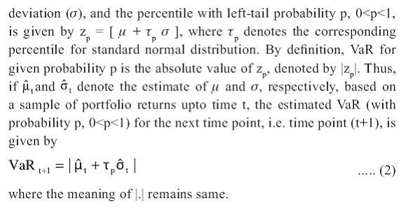 3.2 Non-Normality of Unconditional Return Distribution - Estimating VaR The biggest practical problem of measuring VaR, however, is that the observed returns hardly follow normal distribution - the financial market returns are known to exhibit ‘volatility clustering phenomena’ and follow ‘fat-tailed’ (leptokurtic) distribution with possibly substantial asymmetry. The deviation from normality intensifies the complexity in modelling return distribution, hence estimation of required percentiles and VaR numbers. A simple approach to handle non-normality has been to model return distribution non-parametrically, such as, employing the historical simulation approach. The non-parametric techniques do not assume any specific form of the return distribution and are quite robust over alternative distributional forms. Besides, these techniques are easy to understand and pose no difficulty to implement. But inherent limitations of a non-parametric approach is well known. The conventional parametric approaches to deal with nonnormality can be classified under four broad categories; (i) conditional heteroscedastic models - modeling conditional return distribution through RiskMetric approach, ARCH/GARCH or more advanced forms of such models; (ii) fitting suitable non-normal or mixture distribution for unconditional distribution; and (iii) application of extreme value theory (EVT) - modeling either the distribution of extreme return or only the tails of return distribution. 3.2.1 Non-Parametric Approach - Historical Simulation The non-parametric approach, such as, historical simulation (HS), possess some specific advantages over the normal method, as it is not model based, although it is a statistical measure of potential loss. The main benefit is that it can cope with all portfolios that are either linear or non-linear. The method does not assume any specific form of the distribution of price change/return. The method captures the characteristics of the price change distribution of the portfolio, as it estimates VaR based on the distribution actually observed. But one has to be careful in selecting past data. If the past data do not contain highly volatile periods, then HS method would not be able to capture the same. Hence, HS should be applied when one has very large data points to take into account all possible cyclical events. HS method takes a portfolio at a point of time and then revalues the same using the historical price series. Daily returns, calculated based on the price series, are then sorted in an ascending order and find out the required data point at desired percentiles. Linear interpolation can be used to estimate required percentile if it falls in between two data points. Another variant of HS method is a hybrid approach put forward by Boudhoukh, et al. (1997), that takes into account the exponentially weighing approach in HS for estimating the percentiles of the return directly. As described by Boudhoukh et al. (1997, pp. 3), “the approach starts with ordering the returns over the observation period just like the HS approach. While the HS approach attributes equal weights to each observation in building the conditional empirical distribution, the hybrid approach attributes exponentially declining weights to historical returns”. The process is simplified as follows :
3.2.2 Use of Conditional Heteroscedasticity Models 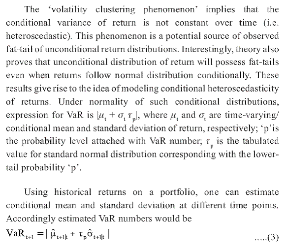 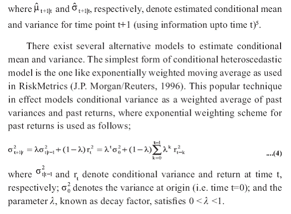 For daily data, the value of the decay parameter in the RiskMetric approach is generally fixed at λ=0.94 (van den Goorberg and Vlaar, 1999). The accuracy in VaR estimates may also improve for alternative values for λ, such as, 0.96 or 0.98 (see for instance, Samanta and Nath, 2004). More advanced models like ARCH, GARCH and so forth (Engle 1982; Bollerslev, 1986; Wong et al., 2003) can also be used for capturing conditional heteroscedasticity. Though conceptually appealing, the performance of the conditional heteroscedastic models in estimating VaR, however, is mixed. In a recent empirical study, Wong et al., (2003) found that the approaches, like, ARCH/GARCH, do not necessarily improve the quality of VaR estimates. 3.2.3 Fitting Non-Normal Distribution for Returns Alternatively, one can simply fit the parametric form of a suitable non-normal distribution to the observed returns. The class of distributional forms considered would be quite wide including, say, hyperbolic distribution, t-distribution, mixture of two or more normal distributions, Laplace distribution or so forth, (van den Goorbergh and Vlaar, 1999; Bauer 2000; Linden, 2001). In our study we consider symmetric hyperbolic distribution as an alternative fat-tailed distribution for returns6. A d-dimensional random variable ‘r’ is said to follow a symmetric hyperbolic distribution if it has density function as below; 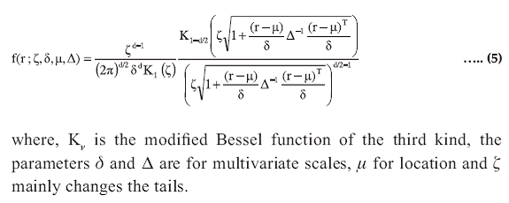 For the presence of Bessel functions in above density function, closed form expression for maximum likelihood estimators are not possible. Bauer (2000) suggests an approach to have maximum likelihood estimators7. Once estimates of the parameters become available, one can estimate the required percentile of the distribution following numerical iteration method. 3.2.4 Methods under Extreme Value Theory – Use of Tail-Index The fat tails of unconditional return distribution can also be handled through extreme value theory using, say, tail-index, which measures the amount of tail fatness. One can therefore, estimate the tail-index and measure VaR based on the underlying distribution. The basic premise of this idea stems from the result that the tails of every fat-tailed distribution converge to the tails of Pareto distribution. In a simple case, upper tail of such a distribution can be modeled as, 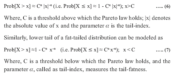 In practice, observations in upper tail of the return distribution are generally positive and those in lower tail are negative. The holder of a short financial position suffers a loss in the event of a rise in values of underlying assets and therefore, concentrates on upper-tail of the distribution (i.e. Eqn. 6) for calculating VaR (Tsay, 2002, pp. 258). Similarly, the holder of a long financial position would model the lower-tail of the underlying distribution (i.e. use Eqn. 7) as a fall in asset values makes her suffer a loss. From Eqns.(6) and (7), it is clear that the estimation of VaR is crucially dependent on the estimation of tail-index α. There are several methods of estimating tail-index, such as, (i) Hill’s (1975) estimator and (ii) the estimator under ordinary least square (OLS) framework suggested by van den Goorbergh and Vlaar (1999). In this study, only the widely used Hill’s estimator of tail-index is considered. Section IV Selecting VaR Model – Evaluation Criteria The accuracy of VaR estimates obtained from a VaR model can be assessed under several frameworks, such as, (i) regulators’ backtesting (henceforth simply called as backtesting); (ii) Kupiec’s test; (iii) loss-function based evaluation criteria. Under each framework, there would be several techniques and what follows is the summary of some of the widely used techniques. 4.1 Backtesting As recommended by Basel Committee, central banks do not specify any VaR model to the banks. Rather under the advanced ‘internal model approach’, banks are allowed to adopt their own VaR model. There is an interesting issue here. As known, VaR is being used for determining minimum required capital – larger the value of VaR, larger is the capital charge. Since larger capital charge may affect profitability adversely, banks have an incentive to adopt a model that produces lower VaR estimate. In order to eliminate such inherent inertia of banks, Basel Committee has set out certain requirements on VaR models used by banks to ensure their reliability (Basel Committee, 1996a,b) as follows ; (i) 1-day and 10-day VaRs must be estimated based on the daily
data of at least one year
(i) One-day VaRs are compared with actual one-day trading
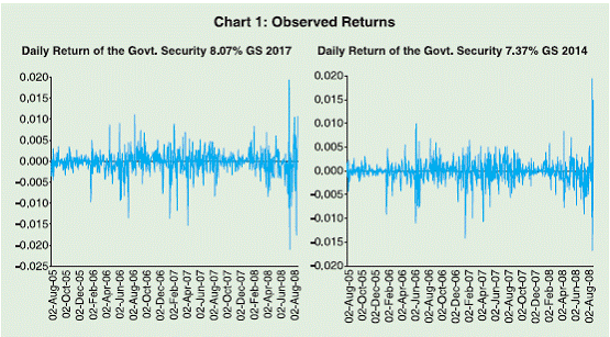
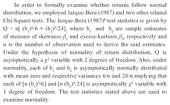
outcomes. (iii) A VaR model fails in Backtesting when it provides 5% or more incorrect VaRs. If a bank provides a VaR model that fails in backtesting, it will have its capital multiplier adjusted upward, thus increasing the amount of capital charges. For carrying out the Backtesting of a VaR model, realized day-to-day returns of the portfolio are compared to the VaR of the portfolio. The number of days, when actual portfolio loss is higher than VaR estimate, provides an idea about the accuracy of the VaR model. For a good 99% VaR model, this number would approximately be equal to the 1 per cent (i.e. 100 times of VaR probability) of backtesting days. If the number of VaR violations or failures (i.e. number of days when observed loss exceeds VaR estimate) is too high, a penalty is imposed by raising the multiplying factor (which is at least 3), resulting in an extra capital charge. The penalty directives provided by the Basel Committee for 250 back-testing trading days is as follows; multiplying factor remains at minimum (i.e. 3) for number of violations up to 4, increases to 3.4 for 5 violations, 3.5 for 6 violations, 3.65 for violations 7, 3.75 for violations 8, 3.85 for violations 9, and reaches at 4.00 for violations above 9 in which case the bank is likely to be obliged to revise its internal model for risk management (van den Goorbergh and Vlaar, 1999). 4.2 Statistical Tests of VaR Accuracy The accuracy of a VaR model can also be assessed statistically by applying Kupiec’s (1995) test (see, for example, van den Goorbergh and Vlaar, 1999 for an application of the technique). The idea behind this test is that frequency of VaR- violation should be statistically consistent with the probability level for which VaR is estimated. Kupiec (1995) proposed to use a likelihood ratio statistics for testing the said hypothesis. If z denotes the number of times the portfolio loss is worse than the VaR estimate in the sample (of size T, say) then z follows a Binomial distribution with parameters (T, p), where p is the probability level of VaR. Ideally, more the z/T closes to p, more accurate the estimated VaR is. Thus the null hypothesis z/T = p may be tested against the alternative hypothesis z/T ≠ p. The likelihood ratio (LR) statistic for testing the null hypothesis against the alternative hypothesis is  Under the null hypothesis, LR-statistic follows a χ2-distribution with 1-degree of freedom. The VaR estimates are also interval forecasts, which thus, can be evaluated conditionally or unconditionally. While the conditional evaluation considers information available at each time point, the unconditional assessment is made without reference to it. The test proposed by Kupiec provides only an unconditional assessment as it simply counts violations over the entire backtesting period (Lopez, 1998). In the presence of time-varying volatility, the conditional accuracy of VaR estimates assumes importance. Any interval forecast ignoring such volatility dynamics may have correct unconditional coverage but at any given time, may have incorrect conditional coverage. In such cases, the Kupiec’s test has limited use as it may classify inaccurate VaR as acceptably accurate. A three-step testing procedure developed by Christoffersen (1998) involves a test for correct unconditional coverage (as Kupiec’s test), a test for ‘independence’, and a test for correct ‘conditional coverage’ (Christoffersen, 1998; Berkowitz and O’Brien, 2002; Sarma, et al., 2003). All these tests use Likelihood-Ratio (LR) statistics. 4.3 Evaluating VaR Models Using Penalty/Loss-Function Tests mentioned above assess the frequency of VaR violations, either conditionally or unconditionally, during the backtesting trading days. These tests, however, do not look at the severity/magnitude of additional loss (i.e. loss in excess of estimated VaR) at the time of VaR violations. However, a portfolio manager may prefer the case of more frequent but little additional loss than the case of less frequent but huge additional loss. The underlying VaR model in the former case may fail in backtesting but still the total amount of loss (after adjusting for penalty on multiplying factor, if any) during the backtesting trading days may be less than that in later case. So long as this condition persists with a VaR model, a portfolio manager, particularly non-banks who are not required to comply with any regulatory requirement, may prefer to accept the VaR model even if it fails in backtesting. This means that the objective function of a portfolio manager is not necessarily be the same as that provided by the backtesting. Each manager may set his own objective function and try to optimize that while managing market risk. But, loss-functions of individual portfolio managers are not available in public domain and thus, it would be impossible to select a VaR model appropriate for all managers. However, discussion on a systematic VaR selection framework by considering a few specific forms of loss-function would provide insight into the issue so as to help individual manager to select a VaR model on the basis of his own loss-function. On this perception, it would be interesting to illustrate the VaR selection framework with the help of some specific forms of loss-function. The idea of using loss-function for selecting VaR model, perhaps, is proposed first by Lopez (1998). He shows that the binomial distribution-based test is actually minimizing a typical loss-function – gives score 1 for a VaR violation and a score 0 otherwise. In other words, the implied loss-function in backtesting would be an indicator function It which assumes a value 1 at time t if the loss at t exceeds corresponding VaR estimate and assumes a value zero otherwise. However, it is hard to imagine an economic agent who has such a utility function: one which is neutral to all times with no VaR violation and abruptly shifts to score of 1 in the slightest failure and penalizes all failures equally (Sarma, et al., 2003). Lopez (1998) also considers a more generalised loss-function which can incorporate the regulatory concerns expressed in the multiplying factor and thus is analogous to the adjustment schedule for the multiplying factor for determining required capital. But, he himself observed that, like the simple binomial distribution-based loss-function, this loss-function is also based on only the number of violations in backtesting observations – with paying no attention to another concern, the magnitudes of loss at the time of failures. In order to handle this situation, Lopez (1998) also proposes a different loss-function addressing the magnitude of violation as follows;  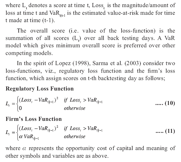 Section V Empirical Results 5.1 Data Data availability in government securities to carry out value-atrisk analy sis is quite difficult. This is simply because the government securities market is still not vibrant, deep and liquid enough. Securities keep on changing their tradability making it difficult to get time series trade data on a particular security for more than, say, three years. One can easily verify that though there are more than ninety outstanding government securities, less than ten securities are traded for good volume or number of trade. Among these, of course, all are not regularly traded. We could get data for three years from August 2005 to July 2008. Effective working days during this three year period was 747 days while the most regularly traded security, 8.07% GS 2017, during this period was traded for 685 days followed by 7.37% GS 2014 for 608 days. Even after having a Primary Dealers system in place, who are specifically treated as market maker, representative quotes or data on that in several government securities are not available. In such a scenario, the analysis was kept limited to the trade data of above mentioned two securities. In case any of these securities is not traded in a particular day, the price has been taken from what is disseminated by Fixed Income Money Market and Derivatives Association of India (FIMMDA) on a daily basis. 5.2 Return Series For each chosen bond, we consider the continuously compounded daily returns computed as follows ; Where Pt and Rt denote the price/value and return in t-th day. Using the price data for 747 days, we have returns on each bond for 746 days. The daily returns, plotted in Chart 1, clearly exhibits volatility clustering indicating the fat-tails of unconditional distribution of returns. Observed probability distribution for each return series also appears to be non-normal (Chart 2). Results of normality tests are presented in Table 1. As can be seen from this table, the Jarque-Bera test statistics is significant at 1% level of significance indicating that none of the return series could be considered to be normally distributed. The Chi-square tests for skewness or excess-kurtosis alone also support the finding. Results on these tests suggest that the underlying return distributions have significant excess-kurtosis indicating presence of fat-tails in the distributions and are skewed, though the degree of asymmetry in the case of the bond 7.37% GS 2014 appears to be mild9
5.3 VaR Estimates from Alternative Techniques. The identified non-normality of the underlying return distributions poses a great difficulty in estimating value-at-risk. As discussed earlier, there have been a plethora of techniques to handle non-normality but hardly any theory can directly identify the best VaR technique for a given portfolio. Thus selecting VaR model is a decision-making problem that has to be addressed empirically. Our strategy in this regard is that estimate VaR using a set of alternative techniques/models and evaluate each competing model based on suitable criteria. In this study, 'normal method' is taken as the benchmark VaR estimation technique. The list of alternative approaches to handle non-normality includes (i) historical simulation – both simple and hybrid; (ii) RiskMetric approach – using exponentially weighted sum of squares of past returns to capture the conditional heteroscedasticity in returns; (iii) symmetric hyperbolic distribution – a distribution having fat-tails; and (iv) tail-index based method – an approach under extreme value theory that measure tail fatness (through tailindex) and model tails of return distribution. As seen earlier, the hybrid/weighted form of historical simulation approach requires a parameter δ, 0 < δ < 1, which determines the weights of past returns while estimating volatility or VaR. As δ takes a fraction value, sometimes fixed at 0.98, the weight decays to with the increase in the remoteness of the past observation/return. We consider three alternative value of δ, viz., 0.94, 0.96 and 0.98. For implementing RiskMetric approach also, there is a need to fix a value for the parameter λ. In original RiskMetric approach, value of this parameter was fixed at 0.94. In this study, however, three alternatives values for λ, viz., 0.94, 0.96 and 0.98 are considered. Table 2 presents estimated 1-day VaRs, with probability level 0.01 (i.e. 99% confidence level), obtained by applying chosen alternative techniques for the last day in our database. Noting that returns do not follow normal distribution, VaR number is likely to be underestimated by normal method. Our empirical results are consistent on this matter. As can be seen from Table 2, VaR estimates obtained from normal method are the lowest for selected bonds10.
Among the non-normal alternatives, historical simulation (simple) and hyperbolic distribution produces the lowest VaR numbers. On the other hand, the RiskMetric and hybrid historical simulation methods produce the highest VaR estimates. The tailindex based method results into VaR estimates some where in between these two sets of estimates. 5.4 Evaluation of Competing VaR Models Competing VaR models were evaluated in terms of their accuracy in estimating VaR over last 447 days in the database. For each VaR model, we followed following steps: First, estimate 1-day VaR with 99% confidence level (i.e. probability level 0.01) using the returns for first 300 days. This estimate is then compared with the loss on 301st day. In case loss exceeds VaR, we say that an instance of VaR-violation has occurred. Second, estimate VaR for 302nd day using returns for past 300 days (covering the period from 2nd to 301st days). This estimate is then compared with the loss in 302nd day in the database to see whether any VaR-violation occurred. Third, the process is repeated until all data points are exhausted. Finally, count the number/percentage of VaR violation over the period of 447 days. For a good VaR model, percentage of VaR violation should be equal to the theoretical value 1% (corresponding with probability level 0.01 of estimated VaR numbers). In Table 3, the number/percentage of VaR violation over last 447 days in the database is given separately for each of the competing VaR models. As can be seen from Table 3, percentage of VaR violation for the benchmark model ‘normal method’ is above 3% - far above the theoretical 1% percentage value. This higher than expected frequency of VaR-violation is attributable to the underestimation of VaR numbers. The RiskMetric and hybrid historical simulation approaches also could not reduce this estimation bias and at times, the frequency of VaR-violation for RiskMetric even exceeds that of the benchmark model. On the other hand, the accuracy level of VaR estimates obtained from ‘hyperbolic distribution’ and ‘tail-index’ methods are much better. In fact, going by the closeness of observed frequency of VaR violation with the theoretical 1% level, the ‘tailindex’ method appears to be producing most accurate VaR numbers followed by the method using ‘hyperbolic distribution’.
In order to see whether the frequency of VaR-violation associated with competing VaR models can be considered as equal to the theoretical 1% value, we employed the popular Kupiec’s test. Relevant empirical results are presented in Table 4. As can be seen from this Table, the hypothesis that the frequency of VaR-violation is equal to the theoretical 1% value could not be accepted at 1% level of significance for the benchmark ‘normal’ method. The results show that the observed frequency is significantly higher than 1%, which indicates that the ‘normal’ method underestimates the VaR number. The Risk Metric approach also could not provide any improvement - the frequency of VaR violation associated with this approach is also statistically higher than 1% value. Thus, like the ‘normal’ method, the Risk Metric approach also underestimates VaR numbers in our case. Interestingly, historical simulation method, in its appropriately chosen form, is able to keep VaR-violation within the statistically acceptable level. However, further improvement is noticeable in estimates of VaR numbers using ‘hyperbolic distribution’ or more so using tail-index method.
The evaluation criteria employed above uses only the frequency of VaR-violation. But the magnitude of VaR violation, defined as the amount of loss in excess of estimated VaR, is also important in evaluating a VaR model. Accordingly, we evaluated value of Lopez’s (1998) loss-function (given by Eqn. 9) for each competing VaR models over the last 446 days in our database. Corresponding results are presented in Table 5. It is seen that the minimum values of loss-function are obtained for ‘tail-index’ method, followed by the ‘hyperbolic distribution’. Historical simulation techniques also have lower loss-function value than the benchmark ‘normal’ method but once again the empirical results indicate that the Risk Metrics not necessarily improves the VaR estimates. Section VI Concluding Remarks In this empirical paper we evaluated a number of competing models/methods for estimating VaR numbers for select Government bonds. Ideally one would like to estimate VaR as a measure of market risk for a much wider real portfolio held by any investor/institute. However, composition of and returns on such a portfolio is not readily available and there also exist certain data limitations. Under such a situation, we chose two most liquid Government bonds during the period from August 2005 to July 2008 and constructed daily return series on the chosen two assets for the period. Though not aimed at analyzing market risk (value-at-risk) of any real bond portfolio, the study is useful in a sense that it demonstrates various relevant issues in details, which can be easily mimicked for any given portfolio. If returns were normally distributed, estimation of VaR would be made simply by using first two moments of the distribution and the tabulated values of standard normal distribution. But the experience from empirical literature shows that the task is potentially difficult for the fact that the financial market returns seldom follow normal distribution. The returns in our database are identified to follow fat-tailed, also possibly skewed, distribution. This observed nonnormality of returns has to be handled suitably while estimating VaR. Accordingly, we employed a number of non-normal VaR models, such as, historical simulation, RiskMetric, hyperbolic distribution fit, method based on tail-index. Our empirical results show that the VaR estimates based on the conventional ‘normal’ method are usually biased downward (lower than actual) and the popular Risk Metric approach could not improve this level of underestimation. Interestingly, historical simulation method (in its suitable chosen form) can estimate VaR numbers more accurately. However, most accurate VaR estimates are obtained from the tail-index method followed by the method based on hyperbolic distribution fit. Notes * Dr. G. P. Samanta, currently a Member of Faculty at Reserve Bank Staff College, Chennai, is Director, Prithwis Jana and Angshuman Hait are Assistant Advisers and Vivek Kumar is Research Officer in the Department of Statistics and Information Management, Reserve Bank of India, Mumbai. Views expressed in the paper are purely personal and not necessarily of the organisation the authors belong to. 1 This means VaR number increases (decreases) with the rise (fall) of confidence level. 2 In the case of market risk, a related view is that ‘holding period’ may be determined from the ‘time required to hedge’ the market risk.  4 It may be noted that the simple HS method corresponds to δ =1, where each of the past k returns is assigned a constant weight 1/k. 5 Conventionally, μt+1|t is considered to be zero, though one can model the return process to have estimates of time-varying/conditional means. 6 The symmetric hyperbolic distribution is a special case of generalized
hyperbolic distribution which depends on six parameters. For a discussion
of hyperbolic distribution, generalized and symmetric, one may see Bauer
(2000).
Select References Artzner, Philippe, Freddy Delbaen, Jean-Marc Eber and David Heath
(1999), Coherent Measures of Risk, Mathematical Finance, Vol. 9, No. 3
(July), pp. 203-28.
Basel Committee (1988), International Convergence of Capital Measurement and Capital Standards - Basel Capital Accord, Bank for International Settlements. Basel Committee (1996a), Amendment to the Capital Accord to Incorporate Market Risks, Bank for International Settlements. Basel Committee (1996b), Supervisory Framework for the Use of ‘Backtesting’ in Conjunction with Internal Models Approach to Market Risk, Bank for International Settlements. Bauer, Christian (2000), “Value at Risk Using Hyperbolic Distributions”, Journal of Economics and Business, Vol. 52, pp. 455-67. Berkowitz, Jeremy and James O’Brien (2002), “How Accurate are Valueat- Risk Models at Commercial Banks?”, Journal of Finance, Vol. LVII, No. 3, June, pp. 1093-111. Bickel, P.J. and K.A. Doksum (1981), “An Analysis of Transformations Revisited”, Journal of American Statistical Association, vol. 76, pp. 296-311. Billio, Monica and Loriana Pelizzon (2000), “Value-at-Risk: A Multivariate Switching Regime Approach”, Journal of Empirical Finance, Vol. 7, pp. 531-54. Bollerslev, T. (1986), “Generalized Autoregressive Conditional Heteroskedasticity”, Journal of Econometrics, Vol. 31, pp. 307-27. Box, G.E.P. and D.R. Cox (1964), “An Analysis of Transformations” (with Discussion), Journal of Royal Statistical Association, Vol. 76, pp. 296-311. Boudoukh J., Matthew Richardson, and R. F. Whitelaw (1997), “The Best of both Worlds: A Hybrid Approach to Calculating Value at Risk”, Stern School of Business, NYU Brooks, Chris and Gita Persand (2003), “Volatility Forecasting for Risk Management”, Journal of Forecasting, Vol. 22, pp. 1-22. Burbidge John B., Lonnie Magee and A. Leslie Robb (1988), “Alternative Transformations to Handle Extreme Values of the Dependent Variable”, Journal of American Statistical Association, March, Vol. 83, No. 401, pp. 123-27. Cebenoyan, A. Sinan and Philio E. Strahan (2004), “Risk Management, Capital Structure and Lending at Banks”, Journal of Banking and Finance, Vol. 28, pp. 19-43. Christoffersen, P.F. (1998), “Evaluating Interval Forecasts”, International Economic Review, 39, pp. 841-62. Christoffersen, P., Jinyong Hahn and Atsushi Inoue (2001), “Testing and Comparing Value-at-Risk Measures”, Journal of Empirical Finance, Vol. 8, No. 3, July, pp. 325-42. Diamond, Douglas W. and Philip H. Dybvig (1983), “Bank Runs, Deposit Insurance, and Liquidity”, Journal of Political Economy, Vol. 91, No. 3, pp. 401-19. Dowd, Kevin. (1998), Beyond Value at Risk: The New Science of Risk Management, (Reprinted, September 1998; January & August 1999; April 2000), Chichester, John Wiley & Sons Ltd. Eberlin, E. and U. Keller (1995), “Hyperbolic Distributions in Finance”, Bernoulli: Official Journal of the Bernoulli Society of Mathematical Statistics and Probability, 1(3), pp. 281-99. Engle, R. F. (1982), “Autoregressive Conditional Heteroscedasticity with Estimates of the Variance of United Kingdom Inflation”, Econometrica, Vol. 50, No. 4, July, pp. 987-1007. Hellmann, Thomas F., Kevin C. Murdock, and Joseph E. Stiglitz (2000), “Liberalisation, Moral Hazard in Banking, and Prudential Regulation: Are Capital Requirements Enough?”, The American Economic Review, Vol. 90, No. 1, Mar, pp. 147-165. Hill, B.M. (1975), “A Simple General Approach to Inference About the Tail of a Distribution”, Annals of Statistics, 35, pp. 1163-73. John, J.A. and N.R.Draper (1980), “An Alternative Family of Transformations”, Appl. Statist., Vol. 29, pp. 190-97. Jorion, Philippe (2001), Value-at-Risk – The New Benchmark for Managing Financial Risk, Second Edition, McGraw Hill. J.P.Morgan/Reuters (1996), RiskMetrics: Technical Document, Fourth Edition, New York, USA. Kupiec, P.(1995), “Techniques for Verifying the Accuracy of Risk Measurement Models”, Journal of Derivatives, Vol. 2, pp. 73-84. Linden, Mikael (2001), “A Model for Stock Return Distribution”, International Journal of Finance and Economics, April, Vol. 6, No. 2, pp. 159-69. Lopez, Jose A. (1998), “Methods for Evaluating Value-at-Risk Estimates”, Federal Reserve Bank of New York Economic Policy Review, October, pp. 119- 124. Mills, Terence C. (1999), The Econometric Modelling of Financial Time Series, 2nd Edition, Cambridge University Press. Nath, Golaka C. and G. P. Samanta (2003), “Value-at-Risk: Concepts and Its Implementation for Indian Banking System”, The Seventh Capital Market Conference, December 18-19, 2003, Indian Institute of Capital Markets, Navi Mumbai, India. Robinson, P. M. and Zaffaroni, P. (1997), "Modelling Nonlinearity and Long Memory in Time Series", Fields Institute Communications, 11, 161–170. Robinson, P. M. and Zaffaroni, P. (1998), "Nonlinear Time Series with Long Memory: A Model for Stochastic Volatility", Journal of Statistical Planning and Inference, 68, 359–371. Samanta, G.P. (2003), “Measuring Value-at-Risk: A New Approach Based on Transformations to Normality”, The Seventh Capital Markets Conference, December 18-19, 2003, Indian Institute of Capital Markets, Vashi, New Mumbai. Samanta, G. P. (2008), "Value-at-Risk using Transformations to Normality: An Empirical Analysis", in Jayaram, N. and R.S.Deshpande [Eds.] (2008), Footprints of Development and Change – Essays in Memory of Prof. V.K.R.V.Rao Commemorating his Birth Centenary, Academic Foundation, New Delhi. The Edited Volume is contributed by the V.K.R.V.Rao Chair Professors at Institute of Social and Economic Change (ISEC), Bangalore, and the scholars who have received the coveted V.K.R.V.Rao Award. Samanta, G.P. and Golaka C. Nath (2004), “Selecting Value-at-Risk Models for Government of India Fixed Income Securities”, ICFAI Journal of Applied Finance, Vol. 10, No. 6, June, pp. 5-29. Sarma, Mandira, Susan Thomas and Ajay Shah (2003), “Selection of Valueat- Risk Models”, Journal of Forecasting, 22(4), pp. 337-358. Taylor, Jeremy, M. G. (1985), “Power Transformations to Symmetry”, Biometrika, Vol. 72, No. 1, pp. 145-52. Tsay, Ruey S. (2002), Analysis of Financial Time Series, Wiley Series in Probability and Statistics, John Wiley & Sons, Inc. van den Goorbergh, R.W.J. and P.J.G. Vlaar (1999), “Value-at-Risk Analysis of Stock Returns Historical Simulation, Variance Techniques or Tail Index Estimation?”, DNB Staff Reports, No. 40, De Nederlandsche Bank. Wong, Michael Chak Sham, Wai Yan Cheng and Clement Yuk Pang Wong (2003), “Market Risk Management of Banks: Implications from the Accuracy of Value-at-Risk Forecasts”, Journal of Forecasting, 22, pp. 23-33. Yeo, In-Kwon and Richard A. Johnson (2000), “A New Family of Power Transformations to Improve Normality or Symmetry”, Biometrika, Vol. 87, No. 4, pp. 954-59. |
||||||||||||||||||||||||||||||||||||||||||||||||||||||||||||||||||||||||||||||||||||||||||||||||||||||||||||||||||||||||||||||||||||||||||||||||||||||||||||||||||||||||||||||||||||||||||||||||||||||||||||||||||||||||||
ପେଜ୍ ଅନ୍ତିମ ଅପଡେଟ୍ ହୋଇଛି:


