 IST,
IST,
RBI WPS (DEPR): 04/2011 : Estimation of Portfolio Value at Risk using Copula
RBI Working Paper Series No. 04 Abstract: *In this paper we use high-frequency multivariate data and attempt to model the joint distribution (dependence structure) of daily exchange rate returns of four major foreign currencies (USD, EURO, GBP and Swiss-Franc) against Indian rupees mainly in the copula-GARCH framework. We also compute 1-day, 99% portfolio Value at Risk (VaR) using Monte Carlo simulation technique for seven multivariate models, which were used to model the dependence structure of the four exchange rate returns. We also compare the performances of these multivariate models based on the goodness of in-sample fit as well as backtesting of VaR results. It is observed that multivariate normal distribution does not fit well the joint distribution of four exchange rate returns under consideration, and also number of exceptions raised in backtesting of VaR estimate are exceptionally high and also unconditional coverage test (binomial test/ kupiec test) and conditional coverage test (christoffersen test) suggest that the VaR estimate is inaccurate. In contrast, VaR estimate based on other six multivariate models produce acceptable VaR estimate. However, among all these seven models Clayton copula model and multivariate student’s t distribution after transforming individual exchange rate returns to student’s t distribution (Hull-White transformation) produce least number of exceptions in back testing of VaR estimate. JEL Classification: C02; C53; C58; G17 Keywords: Copula, GARCH, Exchange rate, Value at Risk (VaR), Monte Carlo Simulation 1. Introduction Recently, the interaction and dependence among the stock markets, exchange rates and interest rates, both locally and cross border, have become stronger than before, mainly on account of greater integration of financial markets, financial innovations, technology innovation which facilitate in massive flow of information among investors and policy makers. A better understanding of the dependence of asset prices is important for proper risk measurement which also helps in deriving full benefit of portfolio diversification by bank/financial analysts. For example, let us assume that the joint distribution of asset prices is skewed, such that there is higher probability of dependence in the left tail than in the right tail. Then, if we assume a symmetric joint distribution to measure the risk (such as value at risk), the assessment will be incorrect since downside and upside risks are different. Value at Risk (VaR) is widely  In this paper we use high-frequency multivariate data and attempt to model the joint distribution (dependency structure) of daily returns of four major foreign currencies (INR-USD, INR-EURO, INR-GBP and INR-CHF) against Indian rupees. Like in many previous works (as discussed in Patton (2002), Alexander et al (2005)), the modelling framework we adopt here is mainly a copula-GARCH model. In particular, we use ARMA-GARCH specification (ARMA for mean specification and GARCH for volatility modeling) to filter the deterministic terms in the daily return series and then model the residuals using number of multivariate statistical models viz. (i) Multivariate normal distribution (ii) Multivariate t-distribution (iii) Converting the individual series so that transformed variables follows Normal distribution (Hull-White transformation) and thereafter fitting these variable to a multivariate normal-distribution. (iv)Transforming the individual series so that transformed variables follows student's t distribution (Hull-White transformation) and thereafter fitting these variable to a multivariate t-distribution. (v) Gauss-copula (vi) Student's t-Copula (vii) Clayton-copula. Thereafter, we compute VaR using Monte Carlo simulation technique for the portfolio with four risk factors (INR-USD, INR-EURO, INR-GBP and INR-CHF exchange rates) of equal weights for each of the seven models of dependency structure as mentioned above. We also compare the performances of these models based on the goodness of in-sample fit (log likelihood values of model fit) to the data as well as back testing of VaR results. 2. Statement of Hypothesis (a) Daily exchange rate returns of the four major foreign currencies against Indian rupees do not follow Gaussian normal distribution. Therefore, using multivariate normal distribution to model the joint distribution of these daily returns is not appropriate and this may lead to inaccurate estimation of VaR of a portfolio of assets which depends on these exchange rates (risk factors). (b) Instead of multivariate normal distribution, copula approach of modeling the dependence structure of daily exchange rate returns would produce comparatively better estimation of VaR of a portfolio of assets which depends on these exchange rates (risk factors). 3. Structure of the paper The paper is organized as follows. Section 4 gives a short literature review on the recent applications of copulas in modeling financial series; Section 5 introduces the modeling dependence structure, where we introduce the copula theory, the copula-GARCH framework and the estimation procedure. In particular, we elaborate seven different multivariate model to model the four exchange rate return series, Section 6 introduces the concept of Value at Risk (VaR) and different techniques to the same, Section 7 describe various methods to compare the performance of models, Section 8 reports estimation results for the seven modeling strategies and makes comparison between them in terms of overall goodness of fit of data and back testing of VaR results and Section 9 concludes. 4. Review of literature Copula is widely used in modeling the joint distributions because it does not require the assumption of joint normality and allow us to decompose n-dimensional joint distribution into its ‘n’ marginal distributions and a copula function which glue them together. Sklar (1959) introduced the term copula. A good introduction to the copula theory may be found in the books of Joe (1997) and Nelsen (1999). The papers of Bouye et al.(2000), Embrechts, Lindskog and McNeil (2003) present general examples of applications of copula in finance. Cherubini and Luciano (2001) estimated the VaR using the Archimedean family copula and the historical empirical distribution to estimate the marginal distributions; Meneguzzo and Vecchiato (2002) used copula for modeling the risk of credit derivatives, Fortin and Kuzmics (2002) used convex linear combinations of copula for estimating the VaR of a portfolio consists of FSTE and DAX stock indices, Embrechts, McNeil and Straumann (2002) and Embrechts, Hoing and Juri (2003) used copula to model extreme value and risk limits. To model the dependence structure between excess returns of "large cap" and "small cap" stock indices, Patton (2004) makes use of a group of frequently used copulas and focuses on the dependence between two stock indices which are more correlated during the market downturn than they are when in the upturn. The deviation from normality could lead to an inadequate VaR estimate and the portfolio could be either riskier than desired or could be needlessly conservative. To measure this asymmetric dependence, the paper uses exceedence correlation, as suggested by Longin & Solnik (2001) and Ang & Chen (2002), and demonstrates that rotated Gumbel copula yields the highest log likelihood (good fit) among all the copula candidates (including both normal and Student’s t copulas) and the same is chosen to model the bivariate distribution of two indices. Long Kang (2007) models the joint distribution of excess returns of four major assets (one year and ten year Treasury bonds and S&P 500 and Nasdaq indices) by a multidimensional copula approach. The modeling framework adopted was a copula-GARCH model where GARCH specification was used to model the marginal distribution of individual assets and then to link the margins together use n-dimensional copula (gauss, t, hierarchical and mixed copula). Nelsen (1998), shows that Archimedean family copula can be used to nest one copula into another copula to form a hierarchical structure. A mixed copula (Tasfack (2006)) is formed by summing up a group of weighted copulas where each copula features dependence between one pair of variables and the sum of the weights is equal to unity. Similar work is also done by Goeij and Marquering (2004) where they model the conditional covariance between stock and bond markets returns by a multivariate GARCH approach. They show strong evidence of heteroskedasticity and asymmetries in the covariance between stock and bond market returns. Tasfack (2006) models dependence structure and extreme co-movements of international equity and bond markets by a regime-switching copula-GARCH model. In one regime, he uses an n-dimensional normal copula to link the marginal distributions and in the other he uses a mixed copula of which each copula component features the dependence structure of a particular pair of variables. The paper empirically demonstrates that dependence between international assets of the same type is high in both regimes while the dependence between equity and bond markets is low even within one country.   (a) Determine the margins F1, ..., Fn, representing the distribution of each factors; estimate their parameters by fitting with the available data. (b) Determine the dependence structure of the random variables X1, ..., Xn, by means of a suitable copula function. Copulas provide greater flexibility in modelling the multivariate distribution by allowing us to fit the appropriate marginal to different random variables and then specifying the appropriate copula function that bind these marginal distributions together. In contrast, traditional representations of multivariate distributions require that all random variables have the same marginal distribution. Since a copula can capture dependence structures regardless of the form of the margins, a copula approach to modelling related variables is potentially very useful in risk management. These advantages imply that copulas provide a superior approach to the modelling of multivariate statistical problems. Example and definition of some of the widely used copula such as Gauss copula, student’s t-copula, Gumbel copula, Clayton copula are given in Annex I. 6. Value at Risk (VaR) In order to compute portfolio VaR, we need to identify basic market rates and prices (risk factors) that affect the value of the portfolio. It is necessary to identify a limited number of basic risk factors; otherwise, the complexity of deriving a portfolio level VaR would be difficult. There are three broad methods to compute VaR i.e. Historical Simulation, Variance-Covariance (Parametric) and Monte Carlo technique. 6.1 Historical Simulation Historical simulation (HS) is simple to implement and requires relatively few assumptions about the statistical distribution of the underlying market factors. HS involves using historical changes in market rates and prices to construct a distribution of potential future portfolio profits and losses and then calculating, for example, the 99%VaR as the loss that is exceeded only 1% of the time. The distribution of profit and losses is constructed by taking the current portfolio and subjecting it to the actual changes in the market factors experienced during each of the last N days (e.g. 250 days). That is N sets of hypothetical values of market factors are constructed using their current values and the changes experienced during the last N periods. Using these hypothetical values of market factors, N hypothetical mark-to-market portfolio values are computed (hypothetical because the current portfolio was not held on each of the last N days). Making use of the actual historical changes in risk factors to compute the hypothetical profits and losses is the important characteristic of historical simulation.  6.3 Monte Carlo Simulation In the case of Monte Carlo technique samples are drawn repeatedly from the random processes governing the prices or returns of the financial instruments we are interested in. For example, if we were interested in estimating a VaR, each simulation would give us a possible value for our portfolio at the end of our holding period. If we take enough of these simulations, the simulated distribution of portfolio values will converge to the portfolio’s unknown ‘true’ distribution, and we can use the simulated distribution of end-period portfolio values to infer the VaR. The simulation process involves a number of specific steps. The first step is to select a model for the stochastic variable(s) of interest. Having chosen our model, we estimate its parameters – volatilities, correlations etc. We then construct the simulated paths for the stochastic variables. Each set of ‘random’ numbers then produces a set of hypothetical terminals price(s) for the instrument(s) in our portfolio. We then repeat these simulations sufficient times to be confident that the simulated distribution of portfolio values to be a reliable proxy for it. Once that is done, we can infer the VaR from this proxy distribution by using quantile / cumulative distribution function/ percentile. In contrast to Historical Simulation, the Parametric VaR model imposes a strong theoretical assumption on the underlying properties of data; frequently Normal Distribution is assumed because it is easily understood and can be defined using only the first two moments. Other probability distributions may be used, but at a higher computational cost. However, empirical evidence indicates that asset price returns, in particular the daily price changes, most of the time does not follow Normal Distribution. In the presence of excess kurtosis, failure rate increases when the VaR is estimated by the Gaussian distribution. As a result, multivariate normal distribution assumption of portfolio is frequently unsatisfactory because large changes occurred more frequently than what is predicted under the normality assumption and which lead to underestimation of the portfolio VaR.    Pearson chi-square normality test suggests that the variables are not normally distributed (Annex II).
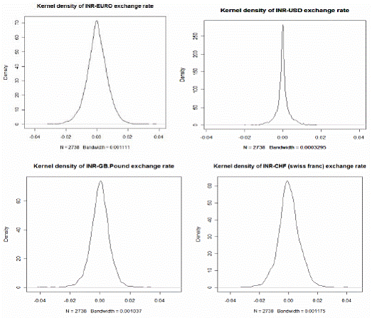
Figure 1: Kernel densities of daily returns of exchange rates
in the portfolio). If we sort these averages (2500) for each of the models separately in descending order 99% VaR would be the 99 percentile of these sorted series. To assess the performance of VaR of these seven models we performed a backtesting for last 200 days (10-Dec-2009 to 27-Sep-2010). 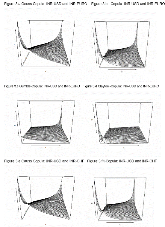 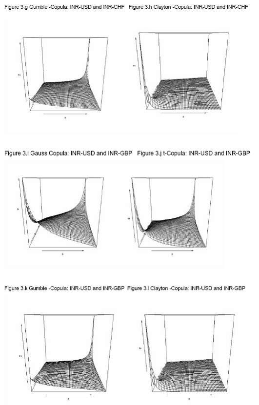 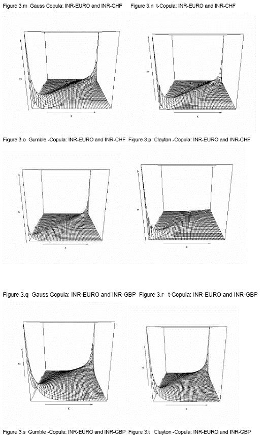 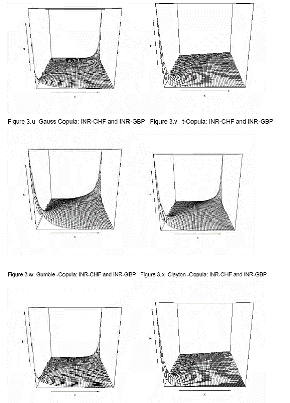 8.3. Comparison of models To compare the goodness of fit and performance of the models we use both the log likelihood values and back testing of results (in terms of number occasion when actual exceed the VaR number). 8.3.1 Log likelihood Estimated parameters and log likelihood values (log likelihood values of copula models are positive and for non-copula models are negative) of all seven models are given in Annex V. Clayton copula and multivariate ‘t’ distribution exhibit best in-sample fit. 8.3.2 Back testing For the purpose of back testing, we use the 200 days data and calculate the number of occurrence of exceptions under each model. Also we compute the Kupiec test and Christoferson test to check the effectiveness of the model. 99% VaR implies that out of 200 days two exceptions are acceptable. The back testing result shows that Model (i) produces 10 exceptions, model (ii), model (iii), model (v) and model (vi) produces three exceptions each and Model (iv) and model (vii) produces two exceptions each. However, Kupiec tests and Christoferson test indicates that for model (i) the null hypothesis is rejected which implies that the VaR estimate using model (i) is not accurate. For all other models null hypothesis cannot be rejected in both the tests. 9. Conclusion In this paper, we use high-frequency multivariate data and attempt to model the joint distribution (dependency structure) of daily returns of four major foreign currencies against Indian rupees. Like in many previous works, the modelling framework we adopt here is mainly a copula-GARCH model. In particular, we use ARMA-GARCH specification to filter the deterministic terms in the daily return series and then model the residuals using various statistical techniques such as (i) multivariate normal distribution; (ii) multivariate t-distribution; (iii) converting the individual series so that transformed variables follows Normal distribution (Hull-White transformation) and thereafter fitting these variable to a multivariate normal-distribution; (iv) transforming the individual series so that transformed variables follows student's t distribution (Hull-White transformation) and thereafter fitting these variable to a multivariate t-distribution; (v) Gauss-copula; (vi) t-Copula; and (vii) Clayton-copula. Thereafter, we compute portfolio VaR using Monte Carlo simulation technique for the portfolio with four risk factors (INR-USD, INR-EURO, INR-GBP and INR-CHF exchange rates) of equal weights for each of the seven models of dependency structure. We also compare the performances of these models based on the log likelihood values of model fit to the data as well as back testing of VaR results. As part of back testing of VaR results, one-day portfolio VaRs were computed for the 200 days for the hypothetical portfolio which depends on these four risk factors using Monte Carlo Simulations technique, for each of the seven models of dependency structure. It is observed that multivariate normal distribution does not provide a good in-sample fit of the joint distribution of four exchange rate returns under consideration, and also number of exceptions raised in backtesting of VaR estimate are exceptionally high and also unconditional coverage test (binomial test/ kupiec test) and conditional coverage test (christoffersen test) suggest that the VaR estimate is inaccurate. In contrast, VaR estimate based on other six models produce acceptable VaR estimate. However, among these models, Clayton copula model (model vii) and multivariate student’s t distribution after transforming individual exchange rate returns to student’s t distribution (Hull-White transformation - model iv) produce least number of exceptions (2 out of 200 days) in back testing of VaR estimate. @Asst. Adviser, Department of Statistics and Information Management, Reserve Bank of India, C-8, Bandra-Kurla Complex, Bandra(E), Mumbai – 400051. email:. *The views expressed in this paper are those of the author alone and not of the institution to which he belongs. References: Alexander J. McNeil, Rudiger Frey, Paul Embrechts, 2005, Quantitative Risk Management: Concepts, Techniques and Tools; Princeton University Press, Princeton and Oxford Ang, A. and J. Chen (2002). Asymmetric Correlations of Equity Portfolios, Journal of Financial Economics 63, 443-494. Bollerslev, T, 1986, "Generalized autoregressive conditional heteroskedasticity". Journal of Econometrics 31:307–327. Bouy´e, E., Durrleman, V., Nikeghbali, A., Riboulet, G. and Roncalli, T. (2000). Copulas for finance, a reading guide and some applications. Working paper, Financial Econometrics Research Centre, City University, London. Cherubini, U. and Luciano, E. (2001). Value at risk trade-off and capital allocation with copulas. Economic Notes 30, 235-256. Clayton, D. G. 1978. "A model for association in bivariate life tables and its application in epidemiological studies of familial tendency in chronic disease incidence.", Biometrika Engle, R. F, 1982, "Autoregressive conditional heteroskedasticity with estimates of the variance of UK inflation.", Econometrica 50:987–1008. Engle, R. F. and T. Bollerslev,1986, "Modeling the persistence of conditional variances.", Econometric Review 5:1–50. Embrechts, P. and Hoing, A., Juri, A. (2003). Using copulae to bound the value-at-risk for functions of dependent risks. Finance and Stochastics 7, 145-167. Embrechts, P., McNeil, A. & Straumann, D. (2001). "Correlation and dependency in risk management: properties and pitfalls. In Risk Management: Value at Risk and Beyond", Cambridge University Press, pp. 176–223. Fortin, I. and Kuzmics, C. (2002). Tail dependence in stock return pairs. International Journal of Intelligent Systems in Accounting, Finance & Management 11, 89-107. Goeij, P., and Wessel Marquering, (2004), "Modeling the Conditional Covariance Between Stock and Bond Returns: A Multivariate GARCH Approach", Journal of Financial econometrics, Vol. 2, No. 4, 531-564. Hamilton, J. 1994. "Time Series Analysis", Princeton University Press. Hull, J. and A. White, 1998, “Value at Risk when Daily Changes in Market Variables are not Normally Distributed,” Journal of Derivatives, Spring 1998, pp 9-19. ----------1998. "Incorporating volatility updating into the historical simulation method for VaR", Journal of Risk 1(1):5–19. ---------- 2001. "Valuing credit default swaps. II. Modelling default correlations", Journal of Derivatives 8(3):12–22. ---------. 2004."Valuation of a CDO and an nth to default CDS without Monte Carlo simulation", Journal of Derivatives 12:8–23. Joe, H. (1997). Multivariate Models and Dependence Concepts. Chapman and Hall. Jorion, P. 2002. "Financial Risk Manager Handbook", 2001–2002.Wiley Jose A. Lopez,1999, "Regulatory Evaluation of Value-at-Risk Models", Research Paper, Research and Market Analysis Group, Federal Reserve Bank of New York. JPMorgan. 1996. "RiskMetrics Technical Documen", 3rd edn. NewYork: JPMorgan. Kupiec, P.,1995,“Techniques for Verifying the Accuracy of Risk Measurement Models,” Journal of Derivatives, 3, 73-84. Longin, F. and Solnik, B. (2001). Extreme correlation of international equity markets. Journal of Finance 56, 649-676. Long Kang (2007), “Modeling the Dependence Structure between Bonds and Stocks: A Multidimensional Copula Approach”, Indiana University Bloomington L¨utkepohl, H. 1993, "Introduction to Multiple Time Series Analysis", 2nd edn. Springer. McNeil, A. J and R. Frey, 2000, "Estimation of tail-related risk measures for heteroskedasticity financial time series: an extreme value approach" Journal of Empirical Finance 7:271–300. Meneguzzo, D. and Vecchiato, W. (2002). Copulas sensitivity in collaterized debt obligations and basket defaults swaps pricing and risk monitoring. Working paper, Veneto Banca. Nelsen, R. B,1998, "An Introduction to Copulas", Springer. Patton, A. J. (2002). Modelling time-varying exchange rate dependence using the conditional copula. Working paper, UCSD. Patton, A. (2003). Modelling asymmetric exchange rate dependence. Working paper, University of California, San Diego. Patton, Andrew J. (2004), "On the Out-of-Sample Importance of Skewness and Asymmetric Dependence for Asset Allocation." Journal of Financial Econometrics, Vol. 2, No. 1, pp. 130-168. Pravin K. Trivedi and David M. Zimmer, 2005, Copula Modeling: An Introduction for Practitioners; Foundations and Trends in Econometrics Vol. 1, No 1 (2005) 1–111 Sklar, A. (1959), "Fonctions de repartition an dimensions et leurs marges", Publications de l’Institut de Statistique de L.Universit de Paris 8, 229-231. Tasfack, Georges (2006), "Dependence Structure and Extreme Comovements in International Equity and Bond Markets”, Working paper, Universite de Montreal, CIRANO and CIREQ. Thomas J. Linsmeier and Neil D. Pearson, 1996, "Risk Measurement: An Introduction to Value at Risk" Zivot, E. and J.Wang. 2003. "Modeling Financial Time Series with S-PLUS", Springer. 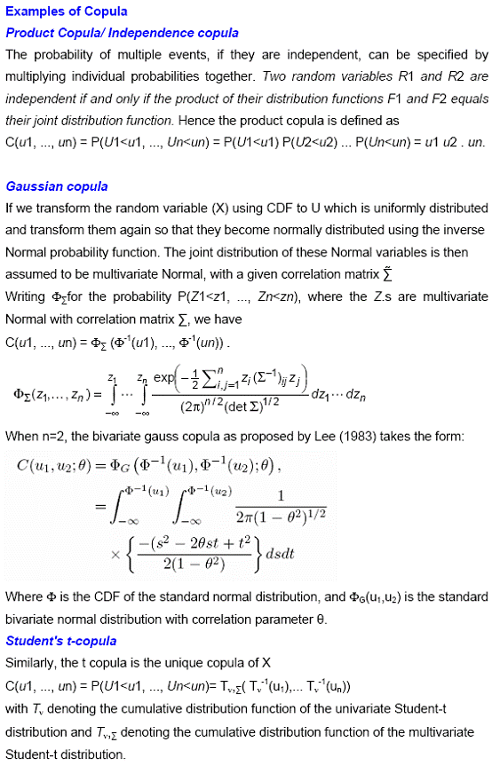 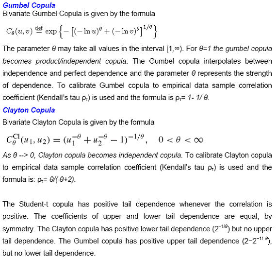 p-value of normality test of exchange rate returns
Annex III Equation 1: GARCH model for INR-CHF daily exchange rate return
Equation 2: GARCH model for INR-EURO daily exchange rate return
Equation 3: GARCH model for INR-GBP daily exchange rate return
Equation 4: GARCH model for INR-USD daily exchange rate return
Annex IV 'R' Script to estimate the parameter of the multivariate distributions, Monte Carlo simulation for VaR computation and back testing the results ('R' version 2.12.0) 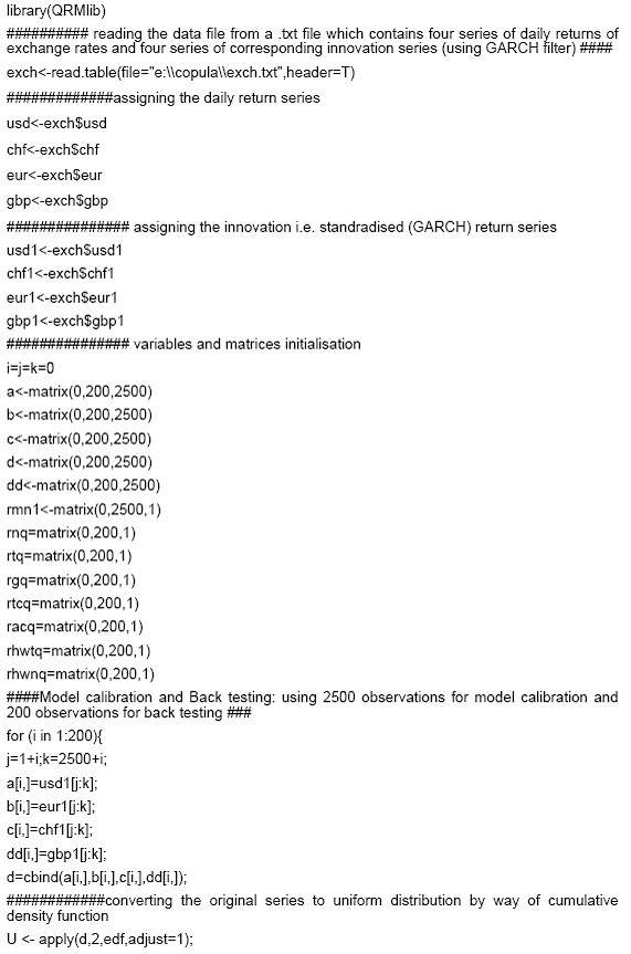 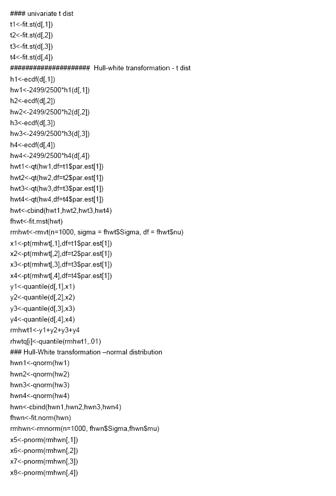 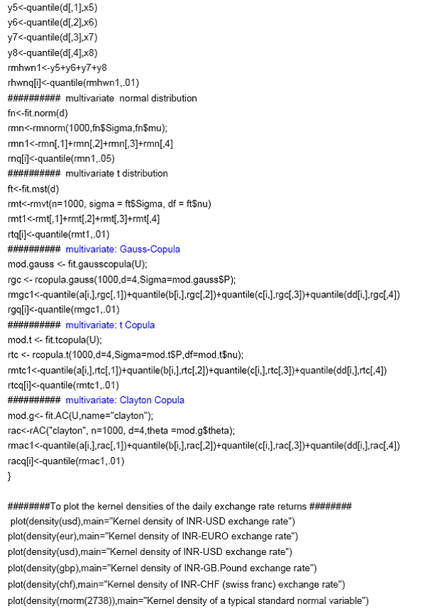 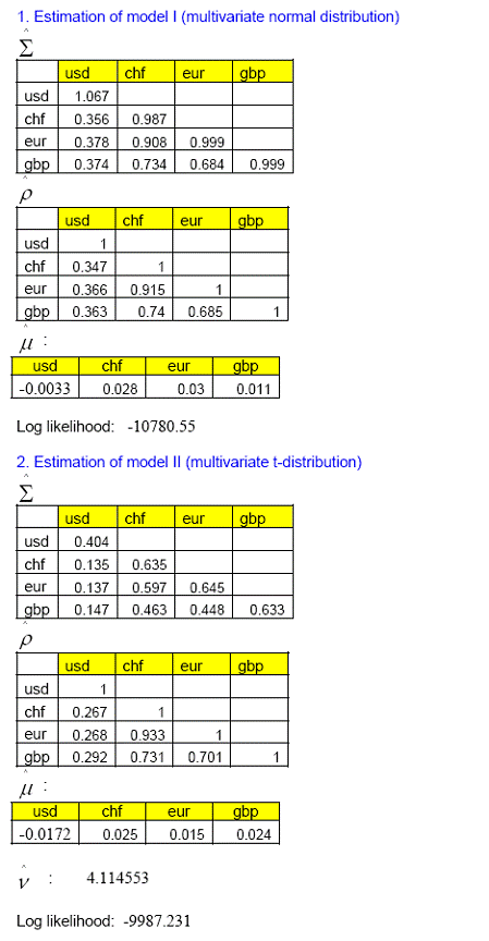 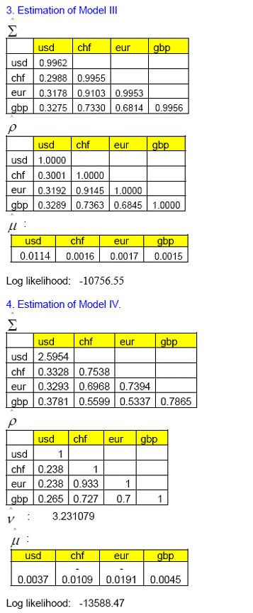 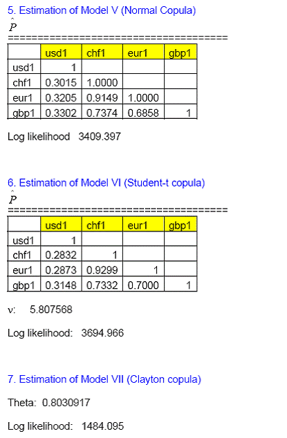 | |||||||||||||||||||||||||||||||||||||||||||||||||||||||||||||||||||||||||||||||||||||||||||||||||||||||||||||||||||||||||||||||||||||||||||||||||||||||||||||||||||||||||||||||||||||||||||||||||||||||||||||||||||||||||||||||||||||||||||||||||||||||||||||||||||||||||||||||||||||||||||||||||||||||||||||||||||||||||||||||||||||||||||||||||||||||||||||||||||||||||||||||||||||||||||||||||||||||||||||||||||||||||||||||||||||||||||||||||||||||||||||||||||||||||||||||||||||||||||||||||||||||||||||||||||||||||||||||||||||||||||||
ପେଜ୍ ଅନ୍ତିମ ଅପଡେଟ୍ ହୋଇଛି:


