Press Release RBI Working Paper Series No. 06 Robust Wald-type Test Statistics based on Minimum C-divergence Estimators @Avijit Maji
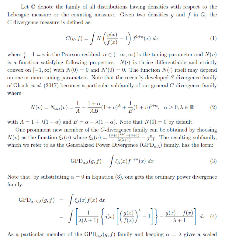
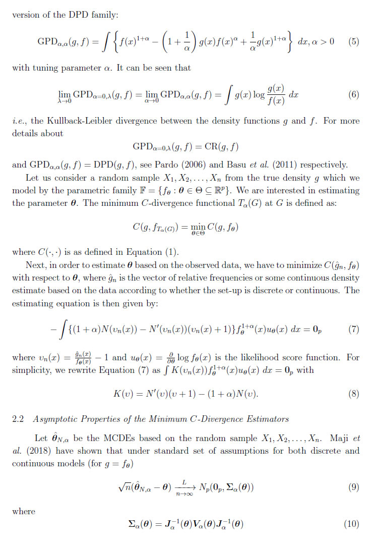
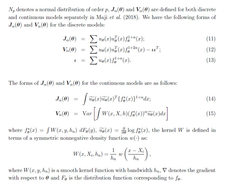
Leandro Pardo Abstract *Recently introduced C-divergence estimators as well as the associated test statis-tics have shown a good robustness behavior. However, one shortcoming of these test statistics is that their asymptotic distribution, in general, is not a chi-square distri-bution but a linear combination of chi-square distributions. In this paper, therefore, we consider Wald-type test statistics based on minimum C-divergence estimators to overcome this shortcoming. We establish that this family of test statistics is a chi-square distribution and compute an approximation of the power function under simple null hypothesis and composite null hypothesis. We calculate both first order and second order influence function of the Wald-type test statistics, based on which the robustness of the family of test statistics can be inferred. Both simulated and real data examples have been shown as part of numerical results. JEL Classification: C12, C13, C15, C18 Keywords: C-divergence, Robust Statistics, Wald-type Test 1. Introduction In the last few years many papers have been published based on minimization of a suitable statistical distance or divergence in order to present robust estimators in para-metric inference as well as robust parametric tests based on them. Many of the statistical distances or divergences are members of the ∅-divergences or the Bregman's distance. In the first case, the most important subfamily is the Cressie and Read (CR) family of di-vergence measures (Pardo, 2006) while in the second case i.e., Bregman distances, the most important family is the density power divergence (DPD) considered for the first time in Basu et al. (1998). Based on these two divergence families (CR and DPD), the C-divergence family was introduced as a generalization of the CR divergence and the DPD (Maji et al., 2018). The minimum C-divergence estimators (MCDEs), based on C-divergence family, manifested substantially superior performance, compared to likeli-hood ratio test, especially in the presence of outliers. On the other hand, without outliers the test statistics were found to be competitive, in general, to the likelihood ratio test. Therefore, the estimators as well as test statistics based on C-divergence measures can serve as useful practical tools in robust statistics. The test statistics based on C-divergence measures, considered in Maji et al. (2018), however, have two small shortcomings. The first is in relation to get the C-divergence measure between two populations in a concrete family of probability distributions. The functional form usually does not boil down to a simpler form and we need to go for numerical methods to evaluate them. While the second one is in relation to the asymptotic distribution of the above test statistics, as in many situations, it is a linear combination of independent chi-squared random variables instead of a chi-squared distribution. It is true that in this moment there are many procedures that can be used while working with linear combination of chi-squared random variables but it is more useful to have a chi-squared distribution as the asymptotic distribution of the test statistics. For similar use of the single chi-squared distribution instead of the linear combination of the chi-squared distributions, see Basu et al. (2016). To overcome the above mentioned issues, we introduce Wald-type tests based on MCDEs in this paper. The architecture of this paper is in similar lines of Basu et al. (2016), but the motivation of the paper differentiates it as well. We show that in this case the asymptotic distribution is a chi-squared distribution and further show that the Wald-type tests based on MCDEs show robust properties. Rest of the paper is organized as follows. Section 2 presents some results obtained in Maji et al. (2018). The Wald-type test statistics based on the MCDEs are analysed in Section 3. The asymptotic distribution is obtained for the simple as well as for the composite null hypothesis in Section 3. Some approximations to the power function are also prescribed in the same section. The influence function of the Wald-type tests based on the MCDEs are obtained in Section 4. A simulation study is carried out in Section 5. Some real data examples are considered in Section 6. A small discussion about the tuning parameter appearing in the Wald-type tests is developed in Section 7. Concluding remarks are in Section 8. 2. Background: The C-Divergence In this section, we pay special attention to the definition of the C-divergence mea-sure, the MCDEs as well as the asymptotic distribution of the MCDEs. 2.1 C-Divergence Measure and the MCDEs
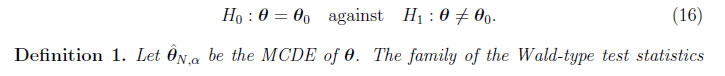
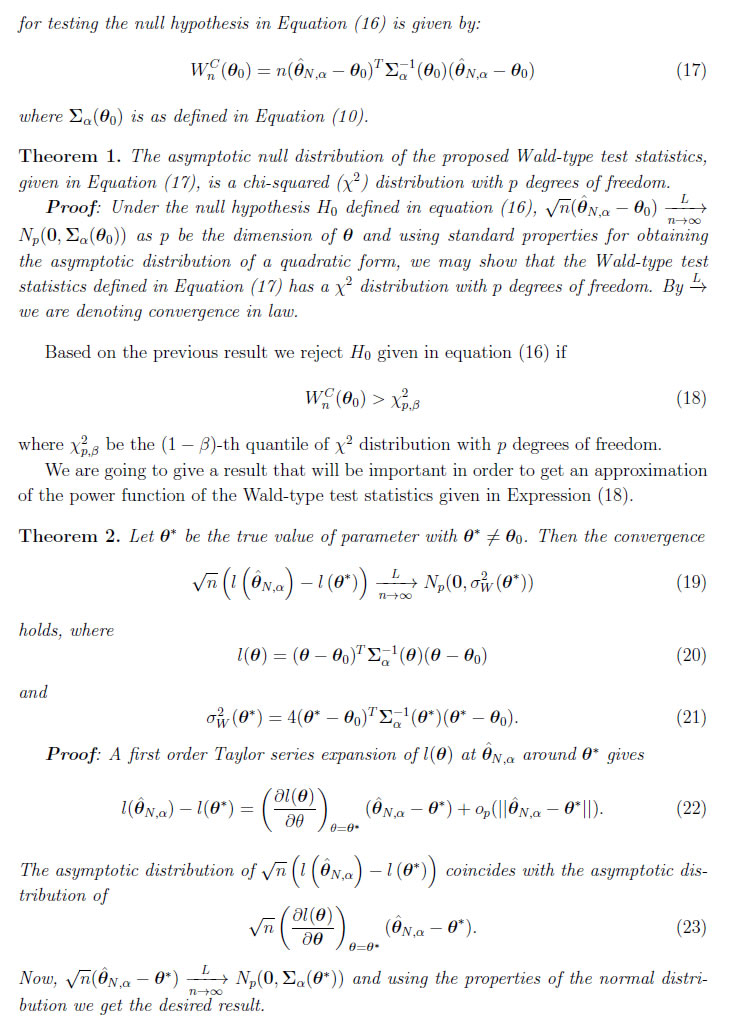
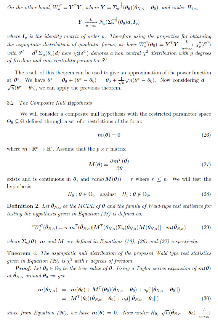
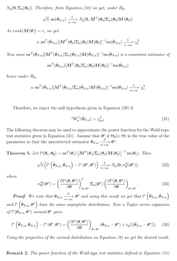
3. Wald-type Tests Based on the MCDE: Definition and Asymptotic Distribution In the last few years it has been very common in the statistical literature to consider Wald tests based on the minimum distance estimators instead of the maximum likelihood estimator. The resulting tests have an excellent behavior in relation to robustness with minimal loss of efficiency (Basu et al., 2016, 2017, 2018 and Ghosh et al. 2016). Based on the results presented in Section 2 we introduce Wald-type test statistics based on the MCDEs in order to test simple and composite null hypothesis. 3.1 The Simple Null Hypothesis We define a family of Wald-type test statistics based on the MCDEs for testing the null hypothesis
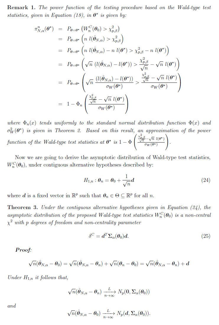
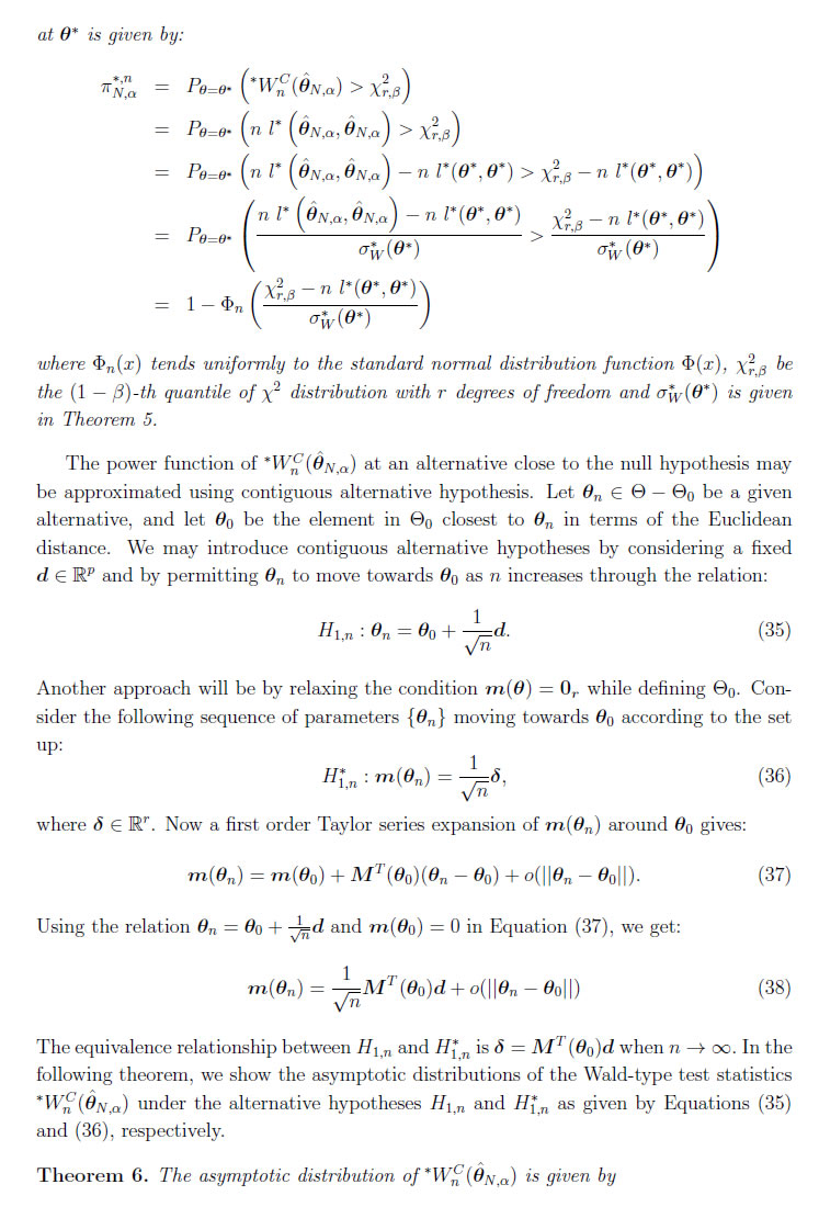
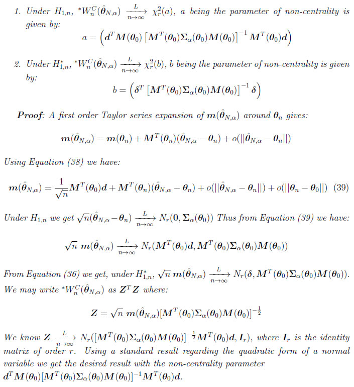
Based on the previous result we can give an approximation to the power function for the testing procedure based on the Wald-type statistics defined in equation (18).
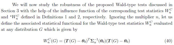
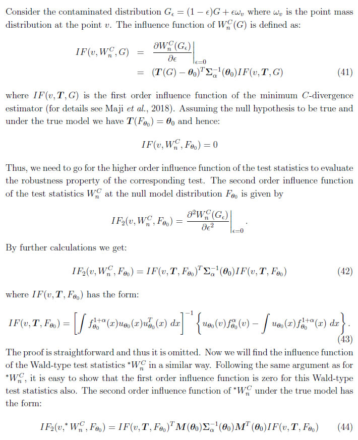
4. Wald-type Tests Based on the MCDE: Robust Results
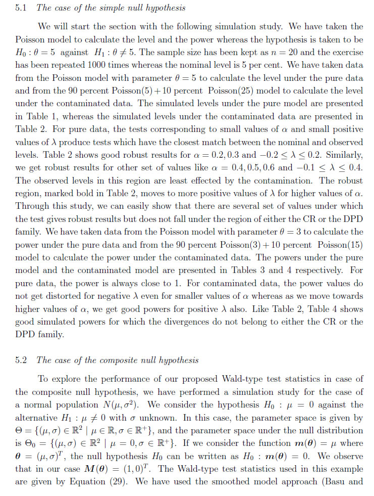
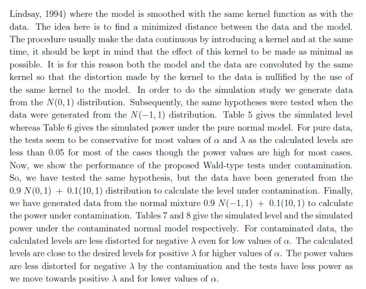
5. Simulation Study In this section, we show simulation analysis using the GPDα,λ family, defined in Equation (3). Maji et al. (2018) have shown that both the CR family (for α = 0) and the DPD family (scaled version for α = λ) may be found as particular members of the GPDα,λ family. We will show that there exist several members of the GPDα,λ family which show good robustness properties but do not belong to either the CR family or the DPD family. Though we have theoretically proved the distributional result, those results are asymptotic in nature. In this section, we show that we may get the desired results for small sample size also.
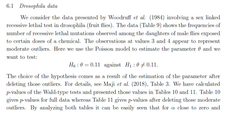
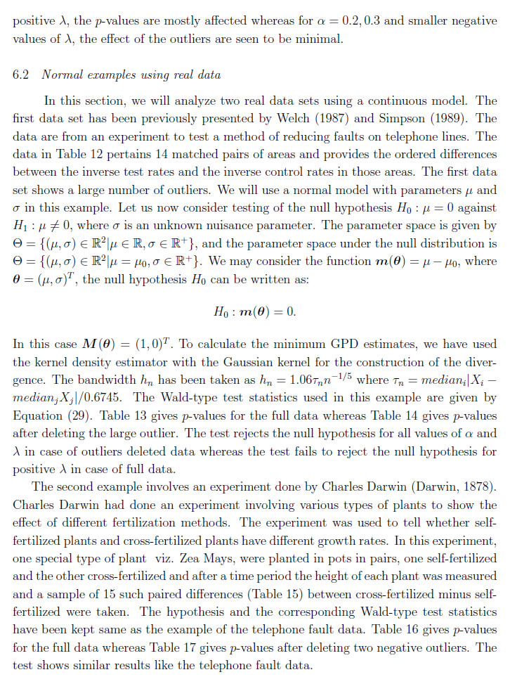
6. Real Data Example
7. Choice of Tuning Parameter In this section, we will restrict ourselves to the GPD family and will not go for the general C-divergence as choice of N(·) requires a separate research. Here we will give some idea to the users regarding the values of the tuning parameters α and λ to be used in practical situations. For pure data, we may use α = λ = 0 as it matches with the likelihood disparity. We may use the data driven approach for contaminated data as we have shown in the above examples. In order to study the overall robustness aspect of the divergence method, we may perform an overall minimization of each of the divergences by considering their tuning parameters to be nuisance parameters varying within a reasonable range. It may be noted that there are several members of the GPD family outside either the CR or the DPD family of divergences which show good robust properties. The region for negative λ and positive α seems to produce good robust results and we usually require high positive value of α for positive λ to get robust results. 8. Conclusion In this paper, we have proposed a Wald-type test based on the minimum C-divergence estimators. We have shown that there exists a direct distributional form of the Wald-type test statistics and have also developed an asymptotic null distribution of the Wald-type test statistics and the approximation of the power function under simple null hypothesis and composite null hypothesis. We have calculated both first order and second order influence function of the Wald-type test statistics. Both simulated and real data example have shown that there exists a region of the parameters for which the tests are found to be robust. We may extend our approach to other divergences.
References [1] Basu, A., A. Ghosh, A. Mandal, N. Martin, and L. Pardo (2017). A Wald-type test statistic for testing linear hypothesis in logistic regression models based on minimum density power divergence estimator. Electronic Journal of Statistics, 11, 2741-2772. [2] Basu, A., A. Ghosh, N. Martin, and L. Pardo (2018). Robust Wald-type tests for non-homogeneous observations based on the minimum density power divergence es-timator. Metrika, 5, 493-522. [3] Basu, A., I. R. Harris, N. L. Hjort, and M. C. Jones (1998). Robust and efficient estimation by minimising a density power divergence. Biometrika, 85, 549-559. [4] Basu, A. and B. G. Lindsay (1994). Minimum disparity estimation for continuous models: Efficiency, distributions and robustness. Annals of the Institute of Statistical Mathematics, 46, 683-705. [5] Basu, A., A. Mandal, N. Martin, and L. Pardo (2016). Generalized Wald-type tests based on minimum density power divergence estimators. Statistics, 1, 1-26. [6] Basu, A., H. Shioya, and C. Park (2011). Statistical Inference: The Minimum Dis-tance Approach. Chapman & Hall/CRC, Boca Raton, FL. [7] Darwin, C. (1878). The Effects of Cross and Self Fertilization in the Vegetable King-dom. John Murray, London. [8] Ghosh, A., I. R. Harris, A. Maji, A. Basu, and L. Pardo (2017). A Generalized Divergence for Statistical Inference. Bernoulli, 23, 2746-2783. [9] Ghosh. A., A. Mandal, N. Martin, and L. Pardo (2016). Influence analysis of robust Wald-type tests. Journal of Multivariate Analysis, 147, 102-126. [10] Maji, A., A. Ghosh, A. Basu, and L. Pardo (2018). Robust statistical inference based on the C-divergence family. Annals of the Institute of Statistical Mathematics, https://doi.org/10.1007/s10463-018-0678-5. [11] Pardo, L. (2006). Statistical Inference based on Divergences. CRC/Chapman-Hall. [12] Simpson, D. G. (1989). Hellinger deviance test: Efficiency, breakdown points, and examples. Journal of the American Statistical Association, 84, 107-113. [13] Welch., W. J. (1987). Rerandomizing the median in matched-pairs designs. Biometrika, 74, 609-614. [14] Woodruff, R. C., J. M. Mason, R. Valencia, and S. Zimmering (1984). Chemical mutagenesis testing in drosophila - I: Comparison of positive and negative control data for sex-linked recessive lethal mutations and reciprocal translocations in three laboratories. Environmental and Molecular Mutagenesis, 6, 189-202.
Annexure | Table 1: Simulated levels of the GPDα,λ Wald-type tests with pure data under the Poisson model (sample size 20) for various values of λ and α; the nominal level is 5%. | | λ ↓ α → | 0 | 0.1 | 0.2 | 0.3 | 0.4 | 0.5 | 0.6 | 0.7 | 0.8 | 0.9 | 1 | | −0.9 | 0.274 | 0.263 | 0.252 | 0.242 | 0.229 | 0.223 | 0.218 | 0.201 | 0.198 | 0.188 | 0.173 | | −0.8 | 0.206 | 0.199 | 0.192 | 0.179 | 0.176 | 0.176 | 0.176 | 0.166 | 0.16 | 0.156 | 0.149 | | −0.7 | 0.143 | 0.146 | 0.143 | 0.145 | 0.142 | 0.143 | 0.149 | 0.146 | 0.141 | 0.139 | 0.134 | | −0.6 | 0.111 | 0.119 | 0.12 | 0.121 | 0.121 | 0.123 | 0.128 | 0.135 | 0.133 | 0.131 | 0.127 | | −0.5 | 0.088 | 0.104 | 0.103 | 0.105 | 0.111 | 0.12 | 0.122 | 0.125 | 0.129 | 0.128 | 0.129 | | −0.4 | 0.074 | 0.082 | 0.098 | 0.101 | 0.1 | 0.102 | 0.109 | 0.115 | 0.114 | 0.118 | 0.122 | | −0.3 | 0.066 | 0.078 | 0.079 | 0.088 | 0.094 | 0.096 | 0.102 | 0.105 | 0.108 | 0.109 | 0.116 | | −0.2 | 0.061 | 0.067 | 0.079 | 0.077 | 0.086 | 0.089 | 0.094 | 0.1 | 0.097 | 0.102 | 0.107 | | −0.1 | 0.055 | 0.061 | 0.075 | 0.076 | 0.08 | 0.084 | 0.084 | 0.092 | 0.097 | 0.097 | 0.1 | | 0 | 0.053 | 0.054 | 0.069 | 0.075 | 0.077 | 0.084 | 0.081 | 0.085 | 0.095 | 0.093 | 0.093 | | 0.1 | 0.05 | 0.051 | 0.057 | 0.069 | 0.074 | 0.075 | 0.079 | 0.082 | 0.087 | 0.092 | 0.09 | | 0.2 | 0.051 | 0.048 | 0.052 | 0.06 | 0.068 | 0.069 | 0.073 | 0.079 | 0.081 | 0.091 | 0.089 | | 0.3 | 0.054 | 0.049 | 0.053 | 0.054 | 0.061 | 0.068 | 0.071 | 0.076 | 0.079 | 0.084 | 0.089 | | 0.4 | 0.057 | 0.051 | 0.05 | 0.052 | 0.056 | 0.063 | 0.066 | 0.07 | 0.076 | 0.082 | 0.082 | | 0.5 | 0.061 | 0.054 | 0.049 | 0.051 | 0.055 | 0.057 | 0.061 | 0.07 | 0.07 | 0.074 | 0.078 | | 0.6 | 0.061 | 0.056 | 0.05 | 0.048 | 0.053 | 0.057 | 0.056 | 0.063 | 0.066 | 0.07 | 0.071 | | 0.7 | 0.068 | 0.058 | 0.053 | 0.048 | 0.049 | 0.055 | 0.052 | 0.055 | 0.063 | 0.066 | 0.068 | | 0.8 | 0.074 | 0.06 | 0.052 | 0.049 | 0.048 | 0.053 | 0.051 | 0.053 | 0.057 | 0.061 | 0.065 | | 0.9 | 0.079 | 0.064 | 0.058 | 0.049 | 0.047 | 0.05 | 0.051 | 0.052 | 0.054 | 0.056 | 0.059 | | 1 | 0.084 | 0.073 | 0.06 | 0.051 | 0.048 | 0.047 | 0.05 | 0.047 | 0.05 | 0.051 | 0.056 |
| Table 2: Simulated levels of the GPDα,λ Wald-type tests with contaminated data under the Poisson model (sample size 20) for various values of λ and α; the nominal level is 5%. | | λ ↓ α → | 0 | 0.1 | 0.2 | 0.3 | 0.4 | 0.5 | 0.6 | 0.7 | 0.8 | 0.9 | 1 | | −0.9 | 0.327 | 0.317 | 0.293 | 0.276 | 0.263 | 0.256 | 0.252 | 0.237 | 0.229 | 0.213 | 0.205 | | −0.8 | 0.243 | 0.241 | 0.233 | 0.226 | 0.217 | 0.206 | 0.196 | 0.187 | 0.181 | 0.174 | 0.171 | | −0.7 | 0.187 | 0.201 | 0.194 | 0.188 | 0.178 | 0.174 | 0.17 | 0.161 | 0.159 | 0.152 | 0.147 | | −0.6 | 0.141 | 0.156 | 0.156 | 0.158 | 0.153 | 0.152 | 0.149 | 0.145 | 0.143 | 0.139 | 0.138 | | −0.5 | 0.12 | 0.127 | 0.129 | 0.13 | 0.135 | 0.132 | 0.129 | 0.127 | 0.125 | 0.12 | 0.118 | | −0.4 | 0.095 | 0.113 | 0.115 | 0.121 | 0.115 | 0.119 | 0.12 | 0.119 | 0.113 | 0.113 | 0.112 | | −0.3 | 0.079 | 0.101 | 0.104 | 0.108 | 0.107 | 0.108 | 0.109 | 0.11 | 0.109 | 0.109 | 0.112 | | −0.2 | 0.086 | 0.102 | 0.094 | 0.099 | 0.101 | 0.103 | 0.104 | 0.105 | 0.105 | 0.104 | 0.105 | | −0.1 | 0.198 | 0.107 | 0.086 | 0.093 | 0.093 | 0.096 | 0.097 | 0.101 | 0.104 | 0.1 | 0.101 | | 0 | 0.698 | 0.134 | 0.086 | 0.08 | 0.081 | 0.089 | 0.093 | 0.094 | 0.099 | 0.096 | 0.098 | | 0.1 | 0.855 | 0.191 | 0.097 | 0.079 | 0.075 | 0.082 | 0.092 | 0.09 | 0.095 | 0.094 | 0.095 | | 0.2 | 0.867 | 0.809 | 0.077 | 0.079 | 0.07 | 0.075 | 0.086 | 0.088 | 0.093 | 0.09 | 0.092 | | 0.3 | 0.87 | 0.858 | 0.739 | 0.069 | 0.074 | 0.071 | 0.079 | 0.081 | 0.09 | 0.088 | 0.089 | | 0.4 | 0.875 | 0.866 | 0.853 | 0.655 | 0.066 | 0.069 | 0.071 | 0.082 | 0.085 | 0.087 | 0.087 | | 0.5 | 0.876 | 0.87 | 0.864 | 0.839 | 0.581 | 0.067 | 0.067 | 0.073 | 0.079 | 0.086 | 0.085 | | 0.6 | 0.877 | 0.875 | 0.868 | 0.859 | 0.816 | 0.516 | 0.065 | 0.067 | 0.071 | 0.08 | 0.083 | | 0.7 | 0.878 | 0.875 | 0.873 | 0.868 | 0.86 | 0.793 | 0.431 | 0.065 | 0.066 | 0.075 | 0.08 | | 0.8 | 0.879 | 0.878 | 0.876 | 0.871 | 0.864 | 0.853 | 0.78 | 0.356 | 0.065 | 0.071 | 0.076 | | 0.9 | 0.879 | 0.879 | 0.876 | 0.874 | 0.868 | 0.865 | 0.845 | 0.755 | 0.305 | 0.066 | 0.073 | | 1 | 0.88 | 0.88 | 0.877 | 0.877 | 0.874 | 0.869 | 0.86 | 0.834 | 0.735 | 0.257 | 0.064 |
| Table 3: Simulated powers of the GPDα,λ Wald-type tests with pure data under the Poisson model (sample size 20) for various values of λ and α; the nominal level is 5%. | | λ ↓ α → | 0 | 0.1 | 0.2 | 0.3 | 0.4 | 0.5 | 0.6 | 0.7 | 0.8 | 0.9 | 1 | | −0.9 | 0.996 | 0.993 | 0.991 | 0.981 | 0.981 | 0.979 | 0.978 | 0.976 | 0.971 | 0.965 | 0.961 | | −0.8 | 0.995 | 0.992 | 0.991 | 0.986 | 0.984 | 0.98 | 0.98 | 0.976 | 0.971 | 0.964 | 0.962 | | −0.7 | 0.998 | 0.994 | 0.992 | 0.989 | 0.987 | 0.984 | 0.976 | 0.973 | 0.97 | 0.969 | 0.964 | | −0.6 | 0.998 | 0.998 | 0.994 | 0.992 | 0.99 | 0.986 | 0.98 | 0.975 | 0.97 | 0.967 | 0.965 | | −0.5 | 0.998 | 0.998 | 0.995 | 0.993 | 0.99 | 0.989 | 0.982 | 0.977 | 0.973 | 0.969 | 0.962 | | −0.4 | 0.998 | 0.998 | 0.998 | 0.993 | 0.992 | 0.989 | 0.98 | 0.976 | 0.975 | 0.969 | 0.961 | | −0.3 | 0.998 | 0.998 | 0.998 | 0.994 | 0.992 | 0.99 | 0.983 | 0.978 | 0.971 | 0.969 | 0.961 | | −0.2 | 0.998 | 0.998 | 0.998 | 0.995 | 0.992 | 0.99 | 0.983 | 0.979 | 0.972 | 0.967 | 0.962 | | −0.1 | 0.998 | 0.998 | 0.998 | 0.996 | 0.994 | 0.989 | 0.984 | 0.979 | 0.974 | 0.967 | 0.963 | | 0 | 0.998 | 0.998 | 0.998 | 0.996 | 0.993 | 0.99 | 0.984 | 0.982 | 0.976 | 0.969 | 0.962 | | 0.1 | 0.997 | 0.998 | 0.998 | 0.995 | 0.995 | 0.99 | 0.986 | 0.982 | 0.978 | 0.97 | 0.961 | | 0.2 | 0.995 | 0.998 | 0.998 | 0.995 | 0.995 | 0.99 | 0.988 | 0.984 | 0.98 | 0.97 | 0.965 | | 0.3 | 0.996 | 0.997 | 0.997 | 0.995 | 0.994 | 0.992 | 0.99 | 0.986 | 0.981 | 0.97 | 0.966 | | 0.4 | 0.994 | 0.994 | 0.996 | 0.995 | 0.994 | 0.992 | 0.992 | 0.987 | 0.982 | 0.973 | 0.968 | | 0.5 | 0.992 | 0.993 | 0.996 | 0.994 | 0.994 | 0.992 | 0.992 | 0.99 | 0.984 | 0.977 | 0.968 | | 0.6 | 0.991 | 0.991 | 0.994 | 0.993 | 0.993 | 0.993 | 0.992 | 0.992 | 0.984 | 0.978 | 0.971 | | 0.7 | 0.989 | 0.992 | 0.992 | 0.992 | 0.992 | 0.993 | 0.992 | 0.99 | 0.987 | 0.981 | 0.971 | | 0.8 | 0.988 | 0.991 | 0.99 | 0.99 | 0.992 | 0.993 | 0.992 | 0.99 | 0.988 | 0.982 | 0.976 | | 0.9 | 0.986 | 0.989 | 0.99 | 0.991 | 0.99 | 0.992 | 0.992 | 0.99 | 0.988 | 0.985 | 0.98 | | 1 | 0.985 | 0.986 | 0.988 | 0.988 | 0.988 | 0.99 | 0.991 | 0.989 | 0.988 | 0.987 | 0.981 |
| Table 4: Simulated powers of the GPDα,λ Wald-type tests with contaminated data under the Poisson model (sample size 20) for various values of λ and α; the nominal level is 5%. | | λ ↓ α → | 0 | 0.1 | 0.2 | 0.3 | 0.4 | 0.5 | 0.6 | 0.7 | 0.8 | 0.9 | 1 | | −0.9 | 0.995 | 0.994 | 0.991 | 0.985 | 0.979 | 0.978 | 0.976 | 0.974 | 0.965 | 0.956 | 0.946 | | −0.8 | 0.996 | 0.995 | 0.992 | 0.989 | 0.983 | 0.979 | 0.977 | 0.972 | 0.965 | 0.957 | 0.945 | | −0.7 | 0.997 | 0.996 | 0.993 | 0.991 | 0.986 | 0.982 | 0.977 | 0.971 | 0.964 | 0.959 | 0.948 | | −0.6 | 0.997 | 0.998 | 0.994 | 0.992 | 0.989 | 0.981 | 0.978 | 0.971 | 0.962 | 0.957 | 0.949 | | −0.5 | 0.993 | 0.999 | 0.996 | 0.992 | 0.991 | 0.985 | 0.979 | 0.971 | 0.963 | 0.957 | 0.946 | | −0.4 | 0.988 | 0.999 | 0.996 | 0.993 | 0.991 | 0.987 | 0.978 | 0.971 | 0.961 | 0.956 | 0.941 | | −0.3 | 0.983 | 0.997 | 0.996 | 0.994 | 0.991 | 0.986 | 0.98 | 0.971 | 0.962 | 0.948 | 0.941 | | −0.2 | 0.948 | 0.994 | 0.997 | 0.994 | 0.991 | 0.986 | 0.98 | 0.973 | 0.961 | 0.947 | 0.938 | | −0.1 | 0.827 | 0.99 | 0.997 | 0.995 | 0.991 | 0.986 | 0.98 | 0.976 | 0.959 | 0.947 | 0.936 | | 0 | 0.54 | 0.976 | 0.993 | 0.995 | 0.991 | 0.988 | 0.982 | 0.974 | 0.958 | 0.945 | 0.934 | | 0.1 | 0.481 | 0.838 | 0.987 | 0.995 | 0.992 | 0.988 | 0.982 | 0.974 | 0.962 | 0.946 | 0.936 | | 0.2 | 0.567 | 0.512 | 0.951 | 0.991 | 0.992 | 0.988 | 0.983 | 0.976 | 0.961 | 0.947 | 0.935 | | 0.3 | 0.609 | 0.529 | 0.582 | 0.972 | 0.988 | 0.987 | 0.982 | 0.977 | 0.962 | 0.95 | 0.936 | | 0.4 | 0.649 | 0.592 | 0.499 | 0.671 | 0.977 | 0.986 | 0.983 | 0.975 | 0.965 | 0.95 | 0.939 | | 0.5 | 0.688 | 0.63 | 0.566 | 0.496 | 0.757 | 0.976 | 0.98 | 0.974 | 0.966 | 0.952 | 0.941 | | 0.6 | 0.72 | 0.67 | 0.607 | 0.54 | 0.512 | 0.808 | 0.971 | 0.972 | 0.965 | 0.951 | 0.94 | | 0.7 | 0.743 | 0.69 | 0.648 | 0.597 | 0.517 | 0.536 | 0.855 | 0.966 | 0.967 | 0.956 | 0.941 | | 0.8 | 0.757 | 0.729 | 0.683 | 0.625 | 0.572 | 0.496 | 0.556 | 0.877 | 0.959 | 0.958 | 0.944 | | 0.9 | 0.774 | 0.748 | 0.699 | 0.664 | 0.609 | 0.558 | 0.495 | 0.574 | 0.891 | 0.952 | 0.946 | | 1 | 0.786 | 0.76 | 0.732 | 0.686 | 0.643 | 0.597 | 0.541 | 0.501 | 0.586 | 0.901 | 0.949 |
| Table 5: Simulated levels of the GPDα,λ Wald-type tests with pure data under the normal model (sample size 20) for various values of λ and α; the nominal level is 5%. | | λ ↓ α → | 0 | 0.1 | 0.2 | 0.3 | 0.4 | 0.5 | 0.6 | 0.7 | 0.8 | 0.9 | 1 | | −0.9 | 0.048 | 0.046 | 0.04 | 0.037 | 0.036 | 0.035 | 0.033 | 0.032 | 0.031 | 0.029 | 0.026 | | −0.8 | 0.043 | 0.042 | 0.037 | 0.038 | 0.037 | 0.037 | 0.034 | 0.033 | 0.031 | 0.028 | 0.026 | | −0.7 | 0.04 | 0.041 | 0.037 | 0.039 | 0.038 | 0.037 | 0.035 | 0.034 | 0.034 | 0.029 | 0.028 | | −0.6 | 0.04 | 0.042 | 0.038 | 0.039 | 0.039 | 0.037 | 0.035 | 0.034 | 0.034 | 0.031 | 0.028 | | −0.5 | 0.041 | 0.043 | 0.038 | 0.039 | 0.038 | 0.037 | 0.036 | 0.035 | 0.034 | 0.032 | 0.029 | | −0.4 | 0.041 | 0.044 | 0.039 | 0.042 | 0.038 | 0.037 | 0.037 | 0.035 | 0.033 | 0.031 | 0.031 | | −0.3 | 0.041 | 0.044 | 0.041 | 0.043 | 0.038 | 0.037 | 0.037 | 0.035 | 0.033 | 0.031 | 0.032 | | −0.2 | 0.039 | 0.043 | 0.041 | 0.043 | 0.039 | 0.037 | 0.037 | 0.035 | 0.033 | 0.031 | 0.032 | | −0.1 | 0.039 | 0.042 | 0.041 | 0.045 | 0.039 | 0.037 | 0.038 | 0.035 | 0.033 | 0.031 | 0.031 | | 0 | 0.039 | 0.041 | 0.041 | 0.045 | 0.039 | 0.037 | 0.038 | 0.035 | 0.033 | 0.031 | 0.031 | | 0.1 | 0.039 | 0.039 | 0.04 | 0.045 | 0.04 | 0.037 | 0.037 | 0.035 | 0.034 | 0.031 | 0.031 | | 0.2 | 0.039 | 0.039 | 0.039 | 0.045 | 0.039 | 0.037 | 0.037 | 0.035 | 0.034 | 0.031 | 0.031 | | 0.3 | 0.039 | 0.039 | 0.039 | 0.042 | 0.04 | 0.037 | 0.037 | 0.034 | 0.034 | 0.032 | 0.03 | | 0.4 | 0.04 | 0.039 | 0.038 | 0.041 | 0.039 | 0.037 | 0.037 | 0.034 | 0.034 | 0.032 | 0.03 | | 0.5 | 0.04 | 0.039 | 0.039 | 0.039 | 0.039 | 0.037 | 0.037 | 0.034 | 0.034 | 0.032 | 0.03 | | 0.6 | 0.042 | 0.039 | 0.039 | 0.038 | 0.038 | 0.037 | 0.038 | 0.034 | 0.034 | 0.031 | 0.03 | | 0.7 | 0.044 | 0.039 | 0.039 | 0.037 | 0.035 | 0.037 | 0.038 | 0.034 | 0.034 | 0.031 | 0.029 | | 0.8 | 0.047 | 0.042 | 0.04 | 0.036 | 0.034 | 0.036 | 0.038 | 0.034 | 0.034 | 0.031 | 0.029 | | 0.9 | 0.05 | 0.044 | 0.04 | 0.037 | 0.033 | 0.035 | 0.037 | 0.035 | 0.034 | 0.031 | 0.029 | | 1 | 0.054 | 0.046 | 0.04 | 0.039 | 0.032 | 0.035 | 0.035 | 0.035 | 0.033 | 0.031 | 0.029 |
| Table 6: Simulated powers of the GPDα,λ Wald-type tests with pure data under the normal model (sample size 20) for various values of λ and α; the nominal level is 5%. | | λ ↓ α → | 0 | 0.1 | 0.2 | 0.3 | 0.4 | 0.5 | 0.6 | 0.7 | 0.8 | 0.9 | 1 | | −0.9 | 0.998 | 0.998 | 0.998 | 0.995 | 0.991 | 0.985 | 0.985 | 0.983 | 0.98 | 0.976 | 0.972 | | −0.8 | 0.998 | 0.998 | 0.998 | 0.994 | 0.989 | 0.985 | 0.985 | 0.983 | 0.98 | 0.975 | 0.97 | | −0.7 | 0.998 | 0.998 | 0.997 | 0.993 | 0.989 | 0.985 | 0.985 | 0.983 | 0.98 | 0.976 | 0.97 | | −0.6 | 0.997 | 0.997 | 0.996 | 0.992 | 0.989 | 0.985 | 0.985 | 0.983 | 0.98 | 0.976 | 0.971 | | −0.5 | 0.997 | 0.997 | 0.995 | 0.992 | 0.99 | 0.985 | 0.985 | 0.983 | 0.982 | 0.976 | 0.971 | | −0.4 | 0.997 | 0.997 | 0.995 | 0.992 | 0.99 | 0.986 | 0.985 | 0.984 | 0.983 | 0.975 | 0.971 | | −0.3 | 0.997 | 0.995 | 0.995 | 0.992 | 0.99 | 0.987 | 0.985 | 0.984 | 0.982 | 0.975 | 0.971 | | −0.2 | 0.997 | 0.996 | 0.995 | 0.993 | 0.99 | 0.987 | 0.985 | 0.984 | 0.982 | 0.975 | 0.971 | | −0.1 | 0.996 | 0.996 | 0.995 | 0.994 | 0.992 | 0.987 | 0.985 | 0.984 | 0.982 | 0.975 | 0.971 | | 0 | 0.996 | 0.996 | 0.995 | 0.994 | 0.992 | 0.987 | 0.986 | 0.984 | 0.982 | 0.975 | 0.971 | | 0.1 | 0.996 | 0.996 | 0.995 | 0.995 | 0.992 | 0.988 | 0.987 | 0.983 | 0.982 | 0.975 | 0.972 | | 0.2 | 0.996 | 0.996 | 0.995 | 0.995 | 0.992 | 0.988 | 0.987 | 0.984 | 0.982 | 0.975 | 0.972 | | 0.3 | 0.995 | 0.996 | 0.995 | 0.995 | 0.993 | 0.988 | 0.988 | 0.984 | 0.982 | 0.975 | 0.972 | | 0.4 | 0.994 | 0.996 | 0.995 | 0.995 | 0.993 | 0.989 | 0.987 | 0.985 | 0.982 | 0.976 | 0.971 | | 0.5 | 0.994 | 0.996 | 0.995 | 0.995 | 0.993 | 0.99 | 0.987 | 0.985 | 0.982 | 0.979 | 0.971 | | 0.6 | 0.994 | 0.995 | 0.995 | 0.995 | 0.995 | 0.99 | 0.987 | 0.985 | 0.982 | 0.979 | 0.971 | | 0.7 | 0.994 | 0.994 | 0.995 | 0.995 | 0.995 | 0.991 | 0.987 | 0.984 | 0.982 | 0.979 | 0.972 | | 0.8 | 0.994 | 0.994 | 0.995 | 0.995 | 0.995 | 0.991 | 0.988 | 0.985 | 0.983 | 0.979 | 0.972 | | 0.9 | 0.994 | 0.994 | 0.993 | 0.995 | 0.995 | 0.991 | 0.988 | 0.985 | 0.983 | 0.978 | 0.973 | | 1 | 0.994 | 0.994 | 0.993 | 0.995 | 0.995 | 0.991 | 0.988 | 0.985 | 0.983 | 0.979 | 0.974 |
| Table 7: Simulated levels of the GPDα,λ Wald-type tests with contaminated data under the normal model (sample size 20) for various values of λ and α; the nominal level is 5%. | | λ ↓ α → | 0 | 0.1 | 0.2 | 0.3 | 0.4 | 0.5 | 0.6 | 0.7 | 0.8 | 0.9 | 1 | | −0.9 | 0.073 | 0.069 | 0.069 | 0.067 | 0.067 | 0.062 | 0.057 | 0.055 | 0.048 | 0.046 | 0.046 | | −0.8 | 0.071 | 0.07 | 0.071 | 0.067 | 0.066 | 0.062 | 0.057 | 0.054 | 0.047 | 0.046 | 0.046 | | −0.7 | 0.072 | 0.071 | 0.07 | 0.066 | 0.066 | 0.062 | 0.057 | 0.054 | 0.048 | 0.047 | 0.047 | | −0.6 | 0.071 | 0.073 | 0.07 | 0.068 | 0.066 | 0.062 | 0.057 | 0.053 | 0.048 | 0.048 | 0.048 | | −0.5 | 0.071 | 0.073 | 0.069 | 0.067 | 0.065 | 0.062 | 0.057 | 0.053 | 0.049 | 0.048 | 0.048 | | −0.4 | 0.072 | 0.071 | 0.069 | 0.067 | 0.066 | 0.062 | 0.057 | 0.053 | 0.049 | 0.048 | 0.048 | | −0.3 | 0.073 | 0.073 | 0.069 | 0.067 | 0.064 | 0.061 | 0.057 | 0.055 | 0.049 | 0.048 | 0.047 | | −0.2 | 0.077 | 0.071 | 0.069 | 0.067 | 0.065 | 0.063 | 0.057 | 0.055 | 0.049 | 0.048 | 0.047 | | −0.1 | 0.12 | 0.081 | 0.07 | 0.067 | 0.066 | 0.063 | 0.057 | 0.055 | 0.049 | 0.048 | 0.047 | | 0 | 0.176 | 0.095 | 0.071 | 0.067 | 0.066 | 0.063 | 0.057 | 0.055 | 0.049 | 0.048 | 0.047 | | 0.1 | 0.888 | 0.108 | 0.073 | 0.067 | 0.067 | 0.063 | 0.057 | 0.055 | 0.049 | 0.048 | 0.047 | | 0.2 | 0.888 | 0.885 | 0.07 | 0.065 | 0.065 | 0.063 | 0.056 | 0.055 | 0.049 | 0.048 | 0.047 | | 0.3 | 0.888 | 0.887 | 0.873 | 0.065 | 0.066 | 0.061 | 0.056 | 0.055 | 0.049 | 0.047 | 0.047 | | 0.4 | 0.889 | 0.887 | 0.886 | 0.855 | 0.064 | 0.06 | 0.055 | 0.054 | 0.049 | 0.047 | 0.047 | | 0.5 | 0.89 | 0.888 | 0.886 | 0.886 | 0.816 | 0.059 | 0.055 | 0.053 | 0.05 | 0.047 | 0.046 | | 0.6 | 0.89 | 0.888 | 0.886 | 0.886 | 0.885 | 0.765 | 0.055 | 0.053 | 0.049 | 0.047 | 0.046 | | 0.7 | 0.89 | 0.89 | 0.886 | 0.886 | 0.886 | 0.882 | 0.689 | 0.053 | 0.049 | 0.047 | 0.046 | | 0.8 | 0.891 | 0.89 | 0.886 | 0.886 | 0.886 | 0.886 | 0.881 | 0.607 | 0.048 | 0.046 | 0.046 | | 0.9 | 0.891 | 0.89 | 0.887 | 0.886 | 0.886 | 0.886 | 0.886 | 0.88 | 0.508 | 0.045 | 0.044 | | 1 | 0.891 | 0.891 | 0.888 | 0.886 | 0.885 | 0.886 | 0.886 | 0.886 | 0.872 | 0.409 | 0.044 |
| Table 8: Simulated powers of the GPDα,λ Wald-type tests with contaminated data under the normal model (sample size 20) for various values of λ and α; the nominal level is 5%. | | λ ↓ α → | 0 | 0.1 | 0.2 | 0.3 | 0.4 | 0.5 | 0.6 | 0.7 | 0.8 | 0.9 | 1 | | −0.9 | 0.985 | 0.986 | 0.982 | 0.978 | 0.977 | 0.973 | 0.969 | 0.963 | 0.961 | 0.954 | 0.947 | | −0.8 | 0.985 | 0.986 | 0.982 | 0.979 | 0.977 | 0.974 | 0.969 | 0.963 | 0.96 | 0.954 | 0.946 | | −0.7 | 0.986 | 0.987 | 0.982 | 0.979 | 0.977 | 0.974 | 0.969 | 0.962 | 0.96 | 0.954 | 0.946 | | −0.6 | 0.986 | 0.986 | 0.982 | 0.979 | 0.976 | 0.974 | 0.969 | 0.962 | 0.96 | 0.953 | 0.947 | | −0.5 | 0.986 | 0.986 | 0.982 | 0.979 | 0.976 | 0.974 | 0.968 | 0.962 | 0.96 | 0.953 | 0.947 | | −0.4 | 0.985 | 0.985 | 0.982 | 0.979 | 0.976 | 0.973 | 0.968 | 0.963 | 0.96 | 0.954 | 0.947 | | −0.3 | 0.984 | 0.985 | 0.982 | 0.98 | 0.976 | 0.972 | 0.969 | 0.963 | 0.959 | 0.954 | 0.947 | | −0.2 | 0.981 | 0.988 | 0.982 | 0.98 | 0.976 | 0.972 | 0.968 | 0.963 | 0.96 | 0.954 | 0.947 | | −0.1 | 0.958 | 0.988 | 0.981 | 0.98 | 0.976 | 0.972 | 0.968 | 0.963 | 0.96 | 0.955 | 0.948 | | 0 | 0.56 | 0.755 | 0.979 | 0.973 | 0.969 | 0.968 | 0.96 | 0.004 | 0.958 | 0.951 | 0.946 | | 0.1 | 0.523 | 0.695 | 0.977 | 0.967 | 0.963 | 0.965 | 0.959 | 0.956 | 0.956 | 0.946 | 0.945 | | 0.2 | 0.562 | 0.521 | 0.918 | 0.964 | 0.96 | 0.957 | 0.962 | 0.961 | 0.957 | 0.95 | 0.948 | | 0.3 | 0.626 | 0.486 | 0.599 | 0.969 | 0.967 | 0.958 | 0.962 | 0.959 | 0.956 | 0.952 | 0.941 | | 0.4 | 0.651 | 0.484 | 0.491 | 0.707 | 0.967 | 0.969 | 0.964 | 0.959 | 0.955 | 0.95 | 0.947 | | 0.5 | 0.673 | 0.528 | 0.449 | 0.534 | 0.791 | 0.969 | 0.959 | 0.962 | 0.955 | 0.95 | 0.948 | | 0.6 | 0.692 | 0.569 | 0.439 | 0.437 | 0.602 | 0.841 | 0.965 | 0.959 | 0.958 | 0.95 | 0.947 | | 0.7 | 0.716 | 0.618 | 0.463 | 0.416 | 0.464 | 0.67 | 0.876 | 0.956 | 0.955 | 0.948 | 0.944 | | 0.8 | 0.737 | 0.646 | 0.5 | 0.409 | 0.407 | 0.502 | 0.697 | 0.885 | 0.957 | 0.948 | 0.946 | | 0.9 | 0.749 | 0.663 | 0.546 | 0.423 | 0.388 | 0.423 | 0.558 | 0.742 | 0.902 | 0.947 | 0.947 | | 1 | 0.771 | 0.688 | 0.579 | 0.454 | 0.386 | 0.372 | 0.444 | 0.598 | 0.765 | 0.905 | 0.949 |
| Table 9: The Drosophila data | | | Recessive lethal count | | Values | 0 | 1 | 2 | 3 | 4 | ≥ 5 | | Observed Frequency | 23 | 3 | 0 | 1 | 1 | 0 |
| Table 10: Calculated p-value of the GPDα,λ Wald-type tests using the drosophila data (full data) | | λ ↓ α → | 0 | 0.1 | 0.2 | 0.3 | 0.4 | 0.5 | 0.6 | 0.7 | 0.8 | 0.9 | 1 | | −0.9 | 0.39 | 0.382 | 0.521 | 0.681 | 0.829 | 0.958 | 0.932 | 0.84 | 0.761 | 0.696 | 0.641 | | −0.8 | 0.694 | 0.622 | 0.742 | 0.884 | 0.994 | 0.893 | 0.81 | 0.741 | 0.684 | 0.635 | 0.593 | | −0.7 | 0.878 | 0.738 | 0.838 | 0.967 | 0.923 | 0.835 | 0.763 | 0.703 | 0.653 | 0.611 | 0.574 | | −0.6 | 0.974 | 0.806 | 0.888 | 0.992 | 0.887 | 0.804 | 0.737 | 0.683 | 0.637 | 0.599 | 0.565 | | −0.5 | 0.82 | 0.855 | 0.913 | 0.97 | 0.868 | 0.787 | 0.723 | 0.671 | 0.627 | 0.591 | 0.558 | | −0.4 | 0.63 | 0.905 | 0.926 | 0.959 | 0.857 | 0.777 | 0.714 | 0.663 | 0.621 | 0.585 | 0.554 | | −0.3 | 0.401 | 0.98 | 0.936 | 0.956 | 0.852 | 0.771 | 0.708 | 0.658 | 0.616 | 0.581 | 0.55 | | −0.2 | 0.193 | 0.873 | 0.953 | 0.956 | 0.852 | 0.769 | 0.705 | 0.654 | 0.612 | 0.578 | 0.547 | | −0.1 | 0.076 | 0.608 | 0.999 | 0.955 | 0.855 | 0.77 | 0.704 | 0.652 | 0.61 | 0.575 | 0.545 | | 0 | 0.029 | 0.301 | 0.869 | 0.94 | 0.857 | 0.771 | 0.704 | 0.651 | 0.608 | 0.573 | 0.543 | | 0.1 | 0.012 | 0.118 | 0.605 | 0.884 | 0.852 | 0.773 | 0.705 | 0.651 | 0.607 | 0.572 | 0.541 | | 0.2 | 0.006 | 0.046 | 0.309 | 0.737 | 0.825 | 0.772 | 0.707 | 0.651 | 0.607 | 0.57 | 0.54 | | 0.3 | 0.003 | 0.019 | 0.134 | 0.49 | 0.747 | 0.758 | 0.706 | 0.652 | 0.607 | 0.57 | 0.539 | | 0.4 | 0.002 | 0.009 | 0.058 | 0.261 | 0.584 | 0.715 | 0.698 | 0.651 | 0.607 | 0.569 | 0.538 | | 0.5 | 0.001 | 0.005 | 0.027 | 0.127 | 0.377 | 0.614 | 0.672 | 0.647 | 0.606 | 0.569 | 0.537 | | 0.6 | 0.001 | 0.003 | 0.014 | 0.063 | 0.213 | 0.456 | 0.61 | 0.631 | 0.603 | 0.568 | 0.536 | | 0.7 | 0 | 0.002 | 0.008 | 0.033 | 0.115 | 0.294 | 0.499 | 0.593 | 0.593 | 0.566 | 0.536 | | 0.8 | 0 | 0.001 | 0.004 | 0.018 | 0.064 | 0.176 | 0.359 | 0.516 | 0.569 | 0.559 | 0.533 | | 0.9 | 0 | 0.001 | 0.003 | 0.011 | 0.037 | 0.104 | 0.237 | 0.406 | 0.518 | 0.543 | 0.529 | | 1 | 0 | 0.001 | 0.002 | 0.007 | 0.022 | 0.063 | 0.15 | 0.29 | 0.435 | 0.51 | 0.519 |
| Table 11: Calculated p-value of the GPDα,λ Wald-type tests using the drosophila data (outliers deleted data) | | λ ↓ α → | 0 | 0.1 | 0.2 | 0.3 | 0.4 | 0.5 | 0.6 | 0.7 | 0.8 | 0.9 | 1 | | −0.9 | 0.382 | 0.477 | 0.576 | 0.674 | 0.764 | 0.843 | 0.911 | 0.969 | 0.984 | 0.947 | 0.918 | | −0.8 | 0.649 | 0.732 | 0.811 | 0.881 | 0.94 | 0.991 | 0.968 | 0.935 | 0.909 | 0.89 | 0.875 | | −0.7 | 0.789 | 0.857 | 0.918 | 0.971 | 0.985 | 0.949 | 0.92 | 0.898 | 0.881 | 0.868 | 0.859 | | −0.6 | 0.874 | 0.931 | 0.981 | 0.978 | 0.943 | 0.915 | 0.894 | 0.877 | 0.865 | 0.857 | 0.851 | | −0.5 | 0.932 | 0.98 | 0.978 | 0.944 | 0.916 | 0.895 | 0.878 | 0.865 | 0.857 | 0.849 | 0.846 | | −0.4 | 0.973 | 0.984 | 0.949 | 0.921 | 0.898 | 0.881 | 0.866 | 0.856 | 0.85 | 0.845 | 0.842 | | −0.3 | 0.995 | 0.959 | 0.929 | 0.904 | 0.884 | 0.87 | 0.859 | 0.85 | 0.845 | 0.842 | 0.84 | | −0.2 | 0.971 | 0.939 | 0.912 | 0.891 | 0.874 | 0.862 | 0.853 | 0.846 | 0.842 | 0.839 | 0.838 | | −0.1 | 0.951 | 0.922 | 0.899 | 0.88 | 0.866 | 0.855 | 0.847 | 0.842 | 0.839 | 0.837 | 0.836 | | 0 | 0.936 | 0.909 | 0.888 | 0.872 | 0.859 | 0.85 | 0.844 | 0.839 | 0.837 | 0.836 | 0.835 | | 0.1 | 0.922 | 0.899 | 0.879 | 0.865 | 0.854 | 0.846 | 0.841 | 0.837 | 0.835 | 0.834 | 0.835 | | 0.2 | 0.91 | 0.889 | 0.872 | 0.859 | 0.85 | 0.842 | 0.838 | 0.835 | 0.834 | 0.833 | 0.834 | | 0.3 | 0.901 | 0.88 | 0.865 | 0.854 | 0.845 | 0.84 | 0.836 | 0.833 | 0.832 | 0.832 | 0.833 | | 0.4 | 0.892 | 0.874 | 0.86 | 0.849 | 0.842 | 0.837 | 0.833 | 0.832 | 0.831 | 0.831 | 0.832 | | 0.5 | 0.885 | 0.868 | 0.855 | 0.846 | 0.839 | 0.835 | 0.831 | 0.83 | 0.83 | 0.831 | 0.832 | | 0.6 | 0.879 | 0.863 | 0.851 | 0.842 | 0.837 | 0.833 | 0.83 | 0.829 | 0.829 | 0.83 | 0.831 | | 0.7 | 0.873 | 0.858 | 0.847 | 0.84 | 0.834 | 0.83 | 0.829 | 0.828 | 0.829 | 0.829 | 0.831 | | 0.8 | 0.868 | 0.853 | 0.844 | 0.836 | 0.832 | 0.829 | 0.827 | 0.827 | 0.828 | 0.829 | 0.83 | | 0.9 | 0.863 | 0.85 | 0.841 | 0.834 | 0.83 | 0.828 | 0.826 | 0.826 | 0.827 | 0.828 | 0.83 | | 1 | 0.859 | 0.846 | 0.837 | 0.832 | 0.829 | 0.826 | 0.825 | 0.825 | 0.826 | 0.827 | 0.83 |
| Table 12: The Telephone Fault Data | | Pair | 1 | 2 | 3 | 4 | 5 | 6 | 7 | 8 | 9 | 10 | 11 | 12 | 13 | 14 | | Difference | −988 | −135 | −78 | 3 | 59 | 83 | 93 | 110 | 189 | 197 | 204 | 229 | 289 | 310 |
| Table 13: Calculated p-value of the GPD Wald-type tests using the telephone fault data (full data) | | λ ↓ α → | 0 | 0.1 | 0.2 | 0.3 | 0.4 | 0.5 | 0.6 | 0.7 | 0.8 | 0.9 | 1 | | −0.9 | 0 | 0 | 0.001 | 0.001 | 0.001 | 0.002 | 0.002 | 0.003 | 0.004 | 0.005 | 0.006 | | −0.8 | 0.001 | 0 | 0.001 | 0.001 | 0.001 | 0.002 | 0.002 | 0.003 | 0.004 | 0.005 | 0.006 | | −0.7 | 0.001 | 0 | 0.001 | 0.001 | 0.001 | 0.002 | 0.002 | 0.003 | 0.004 | 0.005 | 0.006 | | −0.6 | 0.001 | 0 | 0.001 | 0.001 | 0.001 | 0.002 | 0.002 | 0.003 | 0.004 | 0.005 | 0.006 | | −0.5 | 0.001 | 0 | 0.001 | 0.001 | 0.001 | 0.002 | 0.002 | 0.003 | 0.004 | 0.005 | 0.006 | | −0.4 | 0.001 | 0 | 0.001 | 0.001 | 0.001 | 0.002 | 0.002 | 0.003 | 0.004 | 0.005 | 0.006 | | −0.3 | 0.001 | 0 | 0.001 | 0.001 | 0.001 | 0.002 | 0.002 | 0.003 | 0.004 | 0.005 | 0.006 | | −0.2 | 0.002 | 0 | 0 | 0.001 | 0.001 | 0.002 | 0.002 | 0.003 | 0.004 | 0.005 | 0.006 | | −0.1 | 0 | 0 | 0 | 0.001 | 0.001 | 0.002 | 0.002 | 0.003 | 0.004 | 0.005 | 0.006 | | 0 | 0 | 0 | 0 | 0.001 | 0.001 | 0.002 | 0.002 | 0.003 | 0.004 | 0.005 | 0.006 | | 0.1 | 0.774 | 0.21 | 0 | 0.001 | 0.001 | 0.002 | 0.002 | 0.003 | 0.004 | 0.005 | 0.006 | | 0.2 | 0.865 | 0.518 | 0.002 | 0 | 0.001 | 0.002 | 0.002 | 0.003 | 0.004 | 0.005 | 0.006 | | 0.3 | 0.928 | 0.665 | 0.275 | 0.001 | 0.001 | 0.002 | 0.002 | 0.003 | 0.004 | 0.005 | 0.006 | | 0.4 | 0.974 | 0.759 | 0.479 | 0.133 | 0.001 | 0.001 | 0.002 | 0.003 | 0.004 | 0.005 | 0.006 | | 0.5 | 0.991 | 0.826 | 0.604 | 0.333 | 0.077 | 0.002 | 0.002 | 0.003 | 0.004 | 0.005 | 0.006 | | 0.6 | 0.963 | 0.877 | 0.691 | 0.475 | 0.24 | 0.053 | 0.003 | 0.003 | 0.004 | 0.005 | 0.006 | | 0.7 | 0.941 | 0.918 | 0.757 | 0.576 | 0.378 | 0.184 | 0.041 | 0.003 | 0.004 | 0.005 | 0.006 | | 0.8 | 0.922 | 0.951 | 0.809 | 0.653 | 0.484 | 0.311 | 0.149 | 0.033 | 0.004 | 0.005 | 0.006 | | 0.9 | 0.907 | 0.978 | 0.851 | 0.713 | 0.567 | 0.415 | 0.264 | 0.125 | 0.028 | 0.005 | 0.006 | | 1 | 0.894 | 0.999 | 0.886 | 0.763 | 0.634 | 0.499 | 0.364 | 0.23 | 0.108 | 0.025 | 0.006 |
| Table 14: Calculated p-value of the GPD Wald-type tests using the telephone fault data (outliers deleted data) | | λ ↓ α → | 0 | 0.1 | 0.2 | 0.3 | 0.4 | 0.5 | 0.6 | 0.7 | 0.8 | 0.9 | 1 | | −0.9 | 0.001 | 0.001 | 0.001 | 0.001 | 0.001 | 0.001 | 0.002 | 0.002 | 0.003 | 0.003 | 0.004 | | −0.8 | 0.001 | 0.001 | 0.001 | 0.001 | 0.001 | 0.001 | 0.002 | 0.002 | 0.003 | 0.003 | 0.004 | | −0.7 | 0.001 | 0.001 | 0.001 | 0.001 | 0.001 | 0.002 | 0.002 | 0.002 | 0.003 | 0.003 | 0.004 | | −0.6 | 0.001 | 0.001 | 0.001 | 0.001 | 0.001 | 0.002 | 0.002 | 0.002 | 0.003 | 0.003 | 0.004 | | −0.5 | 0.001 | 0.001 | 0.001 | 0.001 | 0.001 | 0.002 | 0.002 | 0.002 | 0.003 | 0.003 | 0.004 | | −0.4 | 0.001 | 0.001 | 0.001 | 0.001 | 0.001 | 0.002 | 0.002 | 0.002 | 0.003 | 0.003 | 0.004 | | −0.3 | 0.001 | 0.001 | 0.001 | 0.001 | 0.001 | 0.002 | 0.002 | 0.002 | 0.003 | 0.003 | 0.004 | | −0.2 | 0.001 | 0.001 | 0.001 | 0.001 | 0.001 | 0.002 | 0.002 | 0.002 | 0.003 | 0.003 | 0.004 | | −0.1 | 0.001 | 0.001 | 0.001 | 0.001 | 0.001 | 0.002 | 0.002 | 0.002 | 0.003 | 0.003 | 0.004 | | 0 | 0.001 | 0.001 | 0.001 | 0.001 | 0.001 | 0.002 | 0.002 | 0.002 | 0.003 | 0.003 | 0.004 | | 0.1 | 0.001 | 0.001 | 0.001 | 0.001 | 0.001 | 0.002 | 0.002 | 0.003 | 0.003 | 0.003 | 0.004 | | 0.2 | 0.001 | 0.001 | 0.001 | 0.001 | 0.001 | 0.002 | 0.002 | 0.003 | 0.003 | 0.004 | 0.004 | | 0.3 | 0.001 | 0.001 | 0.001 | 0.001 | 0.002 | 0.002 | 0.002 | 0.003 | 0.003 | 0.004 | 0.004 | | 0.4 | 0.001 | 0.001 | 0.001 | 0.001 | 0.002 | 0.002 | 0.002 | 0.003 | 0.003 | 0.004 | 0.004 | | 0.5 | 0.001 | 0.001 | 0.001 | 0.001 | 0.002 | 0.002 | 0.002 | 0.003 | 0.003 | 0.004 | 0.004 | | 0.6 | 0.001 | 0.001 | 0.001 | 0.001 | 0.002 | 0.002 | 0.002 | 0.003 | 0.003 | 0.004 | 0.004 | | 0.7 | 0.001 | 0.001 | 0.001 | 0.001 | 0.002 | 0.002 | 0.002 | 0.003 | 0.003 | 0.004 | 0.004 | | 0.8 | 0.001 | 0.001 | 0.001 | 0.001 | 0.002 | 0.002 | 0.002 | 0.003 | 0.003 | 0.004 | 0.004 | | 0.9 | 0.001 | 0.001 | 0.001 | 0.001 | 0.002 | 0.002 | 0.002 | 0.003 | 0.003 | 0.004 | 0.004 | | 1 | 0.001 | 0.001 | 0.001 | 0.001 | 0.002 | 0.002 | 0.002 | 0.003 | 0.003 | 0.004 | 0.004 |
| Table 15: Darwin's Plant Fertilization Data | | Pair | 1 | 2 | 3 | 4 | 5 | 6 | 7 | 8 | 9 | 10 | 11 | 12 | 13 | 14 | 15 | | Difference | −67 | −48 | 6 | 8 | 14 | 16 | 23 | 24 | 28 | 29 | 41 | 49 | 56 | 60 | 75 |
| Table 16: Calculated p-value of the GPD Wald-type tests using Darwin’s plant fertilization data (full data) | | λ ↓ α → | 0 | 0.1 | 0.2 | 0.3 | 0.4 | 0.5 | 0.6 | 0.7 | 0.8 | 0.9 | 1 | | −0.9 | 0.001 | 0 | 0 | 0 | 0 | 0 | 0 | 0 | 0 | 0 | 0 | | −0.8 | 0.002 | 0 | 0 | 0 | 0 | 0 | 0 | 0 | 0 | 0 | 0 | | −0.7 | 0.003 | 0 | 0 | 0 | 0 | 0 | 0 | 0 | 0 | 0 | 0 | | −0.6 | 0.005 | 0 | 0 | 0 | 0 | 0 | 0 | 0 | 0 | 0 | 0 | | −0.5 | 0.007 | 0.001 | 0 | 0 | 0 | 0 | 0 | 0 | 0 | 0 | 0 | | −0.4 | 0.01 | 0.003 | 0 | 0 | 0 | 0 | 0 | 0 | 0 | 0 | 0 | | −0.3 | 0.012 | 0.004 | 0 | 0 | 0 | 0 | 0 | 0 | 0 | 0 | 0 | | −0.2 | 0.015 | 0.007 | 0.001 | 0 | 0 | 0 | 0 | 0 | 0 | 0 | 0 | | −0.1 | 0.017 | 0.009 | 0.003 | 0 | 0 | 0 | 0 | 0 | 0 | 0 | 0 | | 0 | 0.020 | 0.011 | 0.005 | 0 | 0 | 0 | 0 | 0 | 0 | 0 | 0 | | 0.1 | 0.023 | 0.014 | 0.007 | 0.002 | 0 | 0 | 0 | 0 | 0 | 0 | 0 | | 0.2 | 0.025 | 0.016 | 0.009 | 0.003 | 0 | 0 | 0 | 0 | 0 | 0 | 0 | | 0.3 | 0.028 | 0.019 | 0.011 | 0.005 | 0.001 | 0 | 0 | 0 | 0 | 0 | 0 | | 0.4 | 0.031 | 0.021 | 0.014 | 0.007 | 0.003 | 0 | 0 | 0 | 0 | 0 | 0 | | 0.5 | 0.034 | 0.024 | 0.016 | 0.01 | 0.004 | 0.001 | 0 | 0 | 0 | 0 | 0 | | 0.6 | 0.037 | 0.027 | 0.019 | 0.012 | 0.006 | 0.002 | 0.001 | 0 | 0 | 0 | 0 | | 0.7 | 0.039 | 0.03 | 0.022 | 0.015 | 0.009 | 0.004 | 0.001 | 0 | 0 | 0 | 0 | | 0.8 | 0.042 | 0.032 | 0.024 | 0.017 | 0.011 | 0.006 | 0.003 | 0.001 | 0 | 0 | 0 | | 0.9 | 0.045 | 0.035 | 0.027 | 0.02 | 0.014 | 0.008 | 0.004 | 0.002 | 0.001 | 0 | 0 | | 1 | 0.048 | 0.038 | 0.03 | 0.023 | 0.017 | 0.011 | 0.006 | 0.003 | 0.001 | 0.001 | 0 |
| Table 17: Calculated p-value of the GPD Wald-type tests using Darwin’s plant fertilization data (outliers deleted data) | | λ ↓ α → | 0 | 0.1 | 0.2 | 0.3 | 0.4 | 0.5 | 0.6 | 0.7 | 0.8 | 0.9 | 1 | | −0.9 | 0 | 0 | 0 | 0 | 0 | 0 | 0 | 0 | 0 | 0 | 0 | | −0.8 | 0 | 0 | 0 | 0 | 0 | 0 | 0 | 0 | 0 | 0 | 0 | | −0.7 | 0 | 0 | 0 | 0 | 0 | 0 | 0 | 0 | 0 | 0 | 0 | | −0.6 | 0 | 0 | 0 | 0 | 0 | 0 | 0 | 0 | 0 | 0 | 0 | | −0.5 | 0 | 0 | 0 | 0 | 0 | 0 | 0 | 0 | 0 | 0 | 0 | | −0.4 | 0 | 0 | 0 | 0 | 0 | 0 | 0 | 0 | 0 | 0 | 0 | | −0.3 | 0 | 0 | 0 | 0 | 0 | 0 | 0 | 0 | 0 | 0 | 0 | | −0.2 | 0 | 0 | 0 | 0 | 0 | 0 | 0 | 0 | 0 | 0 | 0 | | −0.1 | 0 | 0 | 0 | 0 | 0 | 0 | 0 | 0 | 0 | 0 | 0 | | 0 | 0 | 0 | 0 | 0 | 0 | 0 | 0 | 0 | 0 | 0 | 0 | | 0.1 | 0 | 0 | 0 | 0 | 0 | 0 | 0 | 0 | 0 | 0 | 0 | | 0.2 | 0 | 0 | 0 | 0 | 0 | 0 | 0 | 0 | 0 | 0 | 0 | | 0.3 | 0 | 0 | 0 | 0 | 0 | 0 | 0 | 0 | 0 | 0 | 0 | | 0.4 | 0 | 0 | 0 | 0 | 0 | 0 | 0 | 0 | 0 | 0 | 0 | | 0.5 | 0 | 0 | 0 | 0 | 0 | 0 | 0 | 0 | 0 | 0 | 0 | | 0.6 | 0 | 0 | 0 | 0 | 0 | 0 | 0 | 0 | 0 | 0 | 0 | | 0.7 | 0 | 0 | 0 | 0 | 0 | 0 | 0 | 0 | 0 | 0 | 0 | | 0.8 | 0 | 0 | 0 | 0 | 0 | 0 | 0 | 0 | 0 | 0 | 0 | | 0.9 | 0 | 0 | 0 | 0 | 0 | 0 | 0 | 0 | 0 | 0 | 0 | | 1 | 0 | 0 | 0 | 0 | 0 | 0 | 0 | 0 | 0 | 0 | 0 | |
 IST,
IST,