 IST,
IST,


RBI WPS (DEPR): 07/2023: Regime-Dependent Determinants of the Uncollateralised Overnight Rate: The Interplay of Operating Procedure and Market Microstructure
| RBI Working Paper Series No. 07 Regime-Dependent Determinants of the Uncollateralised Overnight Rate: Edwin Prabu A Abstract 1 Efficient central bank liquidity management is premised on closely aligning the inter-bank overnight rate – the operating target of monetary policy – to the policy repo rate. However, sporadic shocks emanating from a host of factors – institutional, structural, seasonal and idiosyncratic – can sometimes result in the overnight rate breaching the policy interest rate corridor in either direction. Such instances, although rare, merit a rigorous empirical scrutiny. Motivated by the literature on regime-switch in capital flows and using the LASSO technique for high frequency data analysis, this paper uses multinomial logit analysis to delineate the causal factors that determine the location of the interbank rate vis-à-vis the policy corridor during May 2011 to December 2020. It observes that short-term interest rate expectations within the reserve maintenance period, monetary policy expectations, and liquidity distribution are highly significant in explaining the occassional dip of the WACR below the floor of the policy corridor, while liquidity conditions, along with policy expectations and short-term interest rate expectations within the reserve maintenance period are important for the WACR firming up above the ceiling. The findings are robust even after accounting for rare events in the model. JEL Classification: E52, E58, G15 Keywords: Monetary policy, overnight money market, liquidity management, market microstructure. Introduction In central banking parlance, the daily implementation of monetary policy through appropriate liquidity management operations is commonly known as the monetary policy operating procedure. Liquidity management operations and practices are at the core of the operationalisation of monetary policy – “the plumbing in its architecture” (Patra et al., 2016). While monetary policy is known to suffer from both “inside” and “outside” lags in policy transmission,2 the key challenge for an efficient operating procedure is to minimise the lag in transmitting policy rate signals to the operating target (usually, a short-term interest rate), swiftly and seamlessly. Rapid policy transmission is, however, contingent on accurate assessment of the evolving market dynamics and the proactiveness of the central bank in modulating liquidity conditions in sync with the policy stance. The efficacy of the central bank’s actions is judged by its ability to keep the operating target sufficiently close to the policy rate through judicious liquidity management operations. Explicit provisions in the amended RBI Act, 1934 requires the RBI to communicate and disseminate the changes in monetary policy implementation to the public periodically, thereby enhancing policy transparency under the flexible inflation targeting (FIT) framework. In the Indian context, the weighted average call money rate (WACR), representing the unsecured (without collateral) segment of the overnight money market and reflective of systemic liquidity mismatch, is the operating target in the interest rate corridor framework institutionalised in May 2011 (RBI, 2011). Interest rates on standing facilities under the liquidity adjustment facility (LAF) define the interest rate corridor – the marginal standing facility (MSF) rate as the ceiling, the fixed overnight reverse repo rate as the floor3 and the policy repo rate somewhere in between, which effectively summarises the operating procedure. Once the policy repo rate is announced, liquidity operations are conducted to keep the WACR closely aligned to the repo rate. These liquidity operations, which are premised on an accurate assessment of the anticipated liquidity conditions, are aimed at offsetting any demand-supply mismatch with a view to minimise the deviations of the WACR from the policy repo rate. In this regard, the LAF corridor provides the upper and lower bounds of the tolerance band for WACR movements with zero deviation implying perfect marksmanship. To market participants, the extent of success in this marksmanship in normal times serves as an important metric in judging the efficacy of liquidity management operations. As the WACR acts as the initial trigger of monetary transmission, its response to policy rate changes, liquidity operations and other exogenous variables relevant in the extant operational framework is essential for policy evaluation.4 Moreover, stability in the overnight rate is also crucial as higher volatility in the WACR heightens uncertainty about the cost of liquidity, thus raising the term premium across maturities (Kavediya and Pattanaik, 2018). Although the overnight rate level is governed by the prevailing macroeconomic conditions, its day-to-day variation is largely conditioned by the demand for reserves in the inter-bank market. While banks having surplus funds can lend the excess funds (after complying with reserve requirements) in the inter-bank market, banks facing deficit/ shortfall can borrow to meet their requirements. Even though bilateral trading can address the liquidity deficit/ surplus of an individual bank, aggregate system-wide imbalances are offset solely by the central bank, consistent with the policy stance. Therefore, central bank intervention determines the overnight rate, although transient autonomous factors viz., volatile government cash balances may sometimes overwhelm central bank actions and generate large supply shocks.5 There is a vast literature on advanced economies and a few studies on emerging markets that have analysed the overnight rate’s deviation from the policy rate, commonly referred as the “spread” (Linzert and Schmidt, 2011; Kucuk et al., 2016; and Kumar et al., 2017). In a corridor system, liquidity tightness (abundance) in the market for reserves would harden (soften) the overnight rate above (below) the policy rate in the absence of any intervention by the central bank. In this regard, there are several institutional, seasonal, structural and idiosyncratic factors at play along with central bank liquidity operations which determine the relative position of the overnight rate vis-à-vis the corridor (within/ outside). Therefore, it is apposite to identify the key elements among a multitude of factors that could potentially determine the location of the inter-bank rate. In this regard, this study endeavours to delineate the factors that explain the breaching of the corridor by the WACR in either direction. Using multinomial logit models and following an empirical strategy used in the literature on regime shifts in capital flows (Forbes and Warnock, 2012), we estimate the probability of the call rate breaching the interest rate corridor vis-à-vis it being within the corridor due to several factors, viz., (i) uncertainty about liquidity conditions; (ii) market microstructure issues; (iii) structural changes in the implementation framework of monetary policy; and (iv) banks’ expectations of future interest rates. Specifically, we categorise the three regimes as the WACR (i) hardening above the MSF rate; (ii) being within the corridor; and (iii) softening below the reverse repo rate. The multinomial logit model is deployed to estimate the three-category dependent variable and the empirical findings are interpreted using average marginal effects. The results are robust even after accounting for rare events in the model. The remaining part of the paper is structured in the following manner: Section II presents a theoretical overview of liquidity management and the empirical literature on the key determinants of spread. Section III briefly deliberates on the evolution of the operating procedure in India over time and its salient features. Section IV lays out the data and the empirical methodology and Section V discusses the findings and their implications. The concluding observations are presented in Section VI. II.1 Theoretical Underpinnings II.1 (a) Interbank Market6 Central banks’ optimal choice of the operational framework and their liquidity management strategy is determined by three elements viz., (i) an efficient inter-bank money market which ensures smooth transfer of funds from lenders to borrowers; (ii) ability of central banks to forecast liquidity more presciently than market participants; and (iii) the market’s inability to perfectly anticipate monetary policy changes or the monetary authority’s potential in surprising the market, i.e., a possible “announcement effect” (Bindseil, 2014). As mentioned before, the overnight rate is determined by the interaction of demand and supply in the inter-bank market. Central banks can directly control the supply of bank reserves because (i) their forecasts of autonomous factors are superior; (ii) they can plan and conduct market operations; and (iii) they are cognisant about the future policy path. In practice, the actual intent of the central bank’s actions may be interpreted subjectively by market participants, which creates a signal extraction problem (Bindseil, 2000).7 Under a fractional reserve system, commercial banks have to mandatorily maintain a part of their deposit liabilities (some specified proportion) as reserve requirements with the central bank. In fact, they usually hold such balances more than requirements to meet fund settlement obligations within the banking system. Cumulatively, these two factors determine the demand for bank reserves while the supply of reserves in the inter-bank market is the net impact of autonomous drivers of liquidity and central bank market operations. Since excess reserves are usually non-remunerative, the cost of holding excess reserves – which potentially could have been lent in the inter-bank market – is the overnight interest rate foregone. Thus, banks build-up reserve surpluses (drawdown reserves) in present whenever they expect future overnight rates within the reserve maintenance period to be higher (lower) vis-à-vis current levels. Hence, overnight rates are determined as much by expectations about future liquidity conditions as by prevailing circumstances and past developments. Based on the existing literature (Schaechter, 2001; and Linzert and Schmidt, 2011), bank reserves can be partitioned in terms of flows originating from central bank market operations (discretionary factors) and the remaining exogeneous (autonomous) component. The cumulative primary liquidity generated by central banking functions such as being the currency issuer/ manager and banker to both the government and banks is coined as autonomous liquidity (AL), whereas the liquidity created by the market operations of the central bank is called discretionary liquidity (DL). In terms of the balance sheet of a central bank, AL is the sum of (i) credit to the Government; and (ii) net foreign assets of the central bank minus currency and net other liabilities that are leakages from the banking system (Table 1). 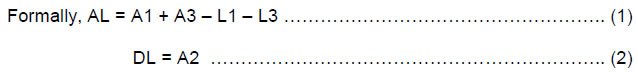 As mentioned before, central banks forecast AL and the total demand for bank reserves (Rd) – the latter can be decomposed into required reserves (RR) and the demand for excess reserves (ERd). Therefore, the ex-ante net systemic liquidity requirement (NL) before central bank market operations can be represented as:  If the central bank decides to maintain the existing liquidity conditions (interest rates), it could compensate NL fully with DL [→ total supply (Rs =AL+DL) = total demand (Rd = RR + ERd)]; if not, interest rates change to clear the inter-bank market. The realised liquidity in the market for bank reserves, ex-post, is simply the banks’ balances maintained with the central bank (L2).  Besides the quantum of liquidity, short-term interest rates also react to changes in the central bank policy rate (ipr) – the price at which liquidity is provided by the central bank to commercial banks. Thus, policy rate changes have a dual impact on the market interest rate – through (i) the instantaneous “announcement effect” and (ii) the “liquidity effect”,8 which are mutually reinforcing. II.1 (b) Corridor versus Floor System As mentioned before, central banks conduct market operations to stabilise the short-term money market rates close to the policy rate. An interest rate corridor is the most common operating procedure wherein the deposit rate – at which commercial banks are remunerated for parking surplus funds with the central bank – represent the floor, while the lending rate – at which the central bank provides funds to commercial banks – constitute the ceiling of the corridor.9 Most often, the key policy rate is in the middle which makes the corridor symmetric. In a floor system, however, the central bank’s deposit rate is the key policy rate. In this scenario, abundant liquidity is infused by the central bank to ensure that the overnight rate is close to the deposit rate. Consequently, an advantage of the floor system is that the central bank can perennially keep systemic liquidity in surplus without pushing overnight market rates below the floor of the corridor. Thus, both the interest rate and the amount of liquidity injected by the central bank act as two independent tools in a floor system (Bernhardsen and Kloster, 2010). 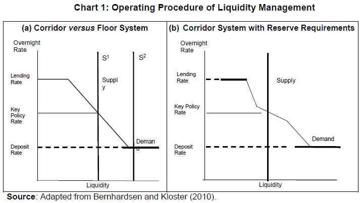 As discussed before, the demand for reserves decline with an increase in the overnight rate. Given demand in the overnight segment, the market clearing rate is determined by the quantum of liquidity supplied. The total supply is determined by the central bank’s discretionary market operations in addition to autonomous factors. As a result, the supply curve is vertical; unresponsive to interest rate changes. In a corridor system, the key policy rate is normally in the middle of the corridor, around which the central bank tries to stabilise overnight market rates (Chart 1 (a)). To achieve this rate, the central bank must provide liquidity given by the supply curve S1 so that supply and demand are equilibrated at that rate. In a floor system, however, the central bank steers the overnight market towards the deposit rate, which becomes the de facto policy rate. In this scenario, the liquidity supply curve is S2, which intersects the demand curve in its flat segment (zero interest rate sensitivity). Augmenting liquidity supply further does not push the overnight rate to dip below the deposit rate. Thus, a liquidity glut in a floor system enables stabilisation of overnight rates close to the key policy rate. Another key difference between a corridor and floor system is the necessity of fine-tuning operations. In a corridor system, any small but random (unanticipated) shocks to demand and supply of liquidity can bring about large changes in the overnight rate. In this scenario, the central bank may have to conduct fine-tuning operations which has to be premised on accurate liquidity forecasts to have the intended effect on overnight rates. In contrast, large shifts in demand and/or supply may not have any impact on overnight rates in a floor system. In a fractional reserve system, however, reserve requirements may check the need for fine-tuning liquidity, based on the statutory requirements for reserve maintenance. If banks are subjected to reserve averaging i.e., they can reduce maintenance to a minimum daily average level over the maintenance period, the demand curve becomes flatter for interest rates near the middle of the corridor (Chart 1 (b)).10 With demand being more elastic, supply changes do not have any noticeable impact on the overnight rate, and hence its volatility is lower. Banks may frontload (backload) their maintenance at the beginning (end) of the maintenance cycle depending on the prevailing market rate and expectation of future rates. If future rates are expected to be lower (higher), banks would presently lend (borrow) aggressively in the interbank market and hold less (more) than the average requirement at the beginning of the maintenance cycle. In the latter half, they would borrow (lend) heavily to meet the shortfall (to deploy the surplus) and hold more (less) than the average daily requirement to fulfil the overall requirement for the entire period. Thus, averaging of reserve requirement acts as an automatic stabiliser in the overnight market (Whitesell, 2006). In contrast to market activity being lukewarm in a floor system, a corridor system facilitates active interbank trading. While the deficit bank eschews borrowing from the central bank and borrows from the interbank market (because it is cheaper), surplus banks want to lend in the overnight market (because it is more remunerative) rather than park the surplus with the central bank. Thus, when the overnight rate is different from those on the central bank’s lending and deposit facilities, the banks seek to avoid using such facilities. On the other hand, as sufficient liquidity is provided by the central bank at a rate marginally above the deposit rate to keep them aligned, it is cost-effective to access the deposit facility in a floor system. Consequently, interbank trading activity dries up as the central bank becomes the sole counterparty for market participants. Finally, policy transmission is highly effective in a corridor system when systemic liquidity is marginally in deficit/ surplus. When such deficits/surplus are large, aligning the overnight rate to the policy rate becomes difficult, even with fine-tuning operations, leading to policy ineffectiveness. In contrast, policy transmission is effective in a floor system as rates can be altered by moving the floor itself, irrespective of the supply of reserves (RBI, 2019). II.2 Empirical Literature A large number of evolving literature related to the overnight market spread has been Euro Area-centric, given that the European Central Bank (ECB) follows a corridor system. The key drivers of the level and the volatility of the European Overnight Rate (EONIA) spread over the ECB’s policy rate are expectations about policy rate changes and liquidity conditions projected for the end period of reserve maintenance (Wurtz, 2003). During the maintenance cycle, the overnight rate is found to be inversely proportional to a permanent change in reserves supply demonstrating a liquidity effect – the magnitude of which is determined by the distribution of liquidity shocks (Moschitz, 2004). In the context of a heterogeneous banking sector, a positive EONIA spread is determined by (i) inter-bank market transaction costs; (ii) total banking sector liquidity requirements; (iii) price of central bank liquidity; and (iv) bank-wise liquidity distribution (Neyer and Wiemers, 2004). In a liquidity framework characterised by money market inefficiencies and banks’ risk aversion, a positive spread can arise primarily because of the uncertainty about liquidity supply from the ECB (Valimaki, 2006). In addition to liquidity conditions and liquidity uncertainty, structural factors such as the ECB’s balance sheet and the operating procedure play a key role in determining the EONIA spread (Linzert and Schmidt, 2011). With increase in EONIA spread’s persistence, the capacity to control the spread may have declined after the ECB introduced the new operational framework in March 2004 (Hassler and Nautz, 2008). Provisioning for long-term liquidity reduced the volatility of the EONIA spread although the spread’s response to liquidity shocks underwent a structural change (Soares and Rodrigues, 2011). Liquidity and credit risk impacted EONIA spread negatively during the global financial crisis (2007-2009), which got largely reflected in money market activity migrating to the overnight segment in the wake of heightened uncertainty (Beirne, 2012). In the ECB’s liquidity auctions conducted after August 2007, a premium was paid by commercial banks which is explained by the interplay between the collateral accepted by the ECB and adverse selection in the interbank market (Casola and Morana, 2008). While evaluating the unconventional monetary policies’ impact on the dynamics of the overnight money market, it is found that the surge in excess reserves: (i) drive overnight rates towards the central bank’s remuneration rate for reserves (i.e., the floor of the corridor); (ii) reduces volatility of the overnight rate; and (iii) dries up activity in the inter-bank market. In addition, counterparty risk affects the pricing of unsecured overnight loans in the inter-bank market even when the banking system is saddled with surplus liquidity (Bech and Monnet, 2013). In an emerging market context, net liquidity deficit, liquidity uncertainty, and liquidity distribution are found to be the most prominent drivers of the overnight spread in Turkey (Kucuk et al., 2016). In the Indian overnight money market, the bid-ask spread was found to be positively associated with the conditional volatility in the call rate prior to 2002. Post-2002, the spread was mainly determined by the conditional variance of the call rate, indicating improved market microstructure (Ghosh and Bhattacharyya, 2009). Net liquidity position as well as total activity in the money market are found to impact the spread between the call rate and the policy repo rate with greater liquidity stress widening the spread. Nevertheless, monetary policy is found to be stable in both excess and deficit liquidity regimes (Nath, 2015). More recently, liquidity deficit, liquidity distribution and liquidity uncertainty are found to have an adverse impact on call money spread in India (Kumar et al., 2017). Both structural and frictional liquidity shocks are found to be crucial in explaining call money rate movements with frictional shocks being more pronounced than structural liquidity shocks. Moreover, interbank call money rates exhibit high volatility persistence, which is attributed to (i) sudden movements in government cash balances; (ii) volatile forex inflows; and (iii) vagaries of currency demand (Singh, 2020). III. Operating Procedure in India III.1 Evolution In India, the evolution of the operating procedure has been in sync with the changing monetary policy framework. With the adoption of a “multiple indicator approach” in 1998, an interim liquidity adjustment facility (ILAF) was introduced in April 1999 which injected liquidity at multiple rates while absorbing it at the fixed rate reverse repo. The shift to a full-fledged liquidity adjustment facility (LAF) in June 2000 resulted in the latter becoming the principal tool for managing liquidity. With the commencement of the LAF, the key challenge of daily liquidity management operations was to steer overnight money market rates in consonance with the objectives of monetary policy (Patra and Kapur, 2012). In turn, policy impulses at the short end were expected to be transmitted across the term structure to long term interest rates, which influence the economy’s spending and investment decisions. In the ensuing years, the repo/ reverse repo rates alternated as the de facto (effective) policy rate based on liquidity deficit/ surplus in the banking system, engendered mostly by large swings in capital flows. Oscillating liquidity conditions resulted in the call money rate turning highly volatile, often breaching the corridor in either direction. Accordingly, modifications in the operating framework in May 2011 made repo rate, the single policy rate (RBI, 2011).11 For liquidity management purposes, the weighted average call rate (WACR) was chosen as the operating target. The objective of liquidity management was to keep the WACR sufficiently close to the repo rate. To provide a safety valve against unanticipated liquidity shocks, a marginal standing facility (MSF) was instituted under which banks could borrow overnight at a premium above the repo rate (Patra et al., 2016). The corridor was re-defined as a symmetric one in which the reverse repo rate and the MSF rate were equidistantly below and above the repo rate. Shortcomings of this framework, however, came to the fore immediately after the taper tantrum of May 2013, the most prominent being (i) excessive reliance of the RBI on the overnight money market segment; and (ii) unrestricted supply of liquidity at the fixed repo rate. In this context, it was suggested by an Expert Committee that liquidity management operations should be conducted through repos of varying maturities (RBI, 2014). Accordingly, a revised framework was introduced in September 2014, the salient features of which were (i) withdrawal of unconstrained liquidity accommodation at the fixed repo rate; (ii) providing liquidity largely through auction-based term repos; (iii) introduction of liquidity fine-tuning operations of different tenors; (iv) withdrawal of export credit refinance; and (v) progressive reduction in the statutory liquidity ratio (SLR). Under this framework, banks had access to fixed rate repo up to 0.25 per cent of their own net demand and time liabilities (NDTL) and up to 0.75 per cent of the banking system NDTL through four 14-day variable rate term repo auctions. Based on periodic liquidity assessment, the Reserve Bank also conducted liquidity fine-tuning operations of varying tenors. As the key instrument for providing liquidity, the 14-day term repo was synchronised with the reserve maintenance cycle thereby allowing market participants to (i) plan their fund requirements for a longer duration; and (ii) develop a medium-term interest rate outlook. This, in turn, was expected to facilitate the emergence of a term money market and develop benchmarks for term transactions. Thus, the Reserve Bank’s liquidity management operations became increasingly proactive and forward-looking than in the earlier system. In April 2016, the framework was further modified with the shift to an accommodative monetary policy stance. The supply of durable liquidity was sought to be smoothened over the year through flexible asset purchases/ sales operations while reducing the average ex-ante systemic liquidity deficit sufficiently close to neutrality. This framework was driven by the dual objectives of (i) injecting or absorbing short term liquidity to offset transient changes in reserves; and, (ii) supplying adequate durable reserves to meet the growing economy’s requirements. While the first objective was met by offsetting frictional mismatches through LAF to keep systemic liquidity closer to neutrality, the second objective was achieved by appropriately tempering the flow of net foreign assets and/ or net domestic assets in the balance sheet of the Reserve Bank as per systemic requirements (e.g., sterilisation operations following forex market interventions).12 Moreover, the policy corridor width was progressively tapered to 50 bps in a symmetric manner by April 2017. Over the next two years, the operating procedure remained broadly unchanged although new instruments were added to the toolkit of liquidity management, e.g., long-term US$ buy/ sell swap in March 2019 to inject durable liquidity. Although the extant framework proved to be resilient, it was rendered complex because of multiple fine-tuning operations. Moreover, liquidity assessment by different market participants varied markedly obfuscating the intent of the Reserve Bank’s liquidity management operations, which necessitated a relook at the existing framework. Based on the findings of an Internal Working Group, the Reserve Bank announced the revised framework with a view to clearly communicate the objectives and the toolkit for liquidity management (RBI, 2020). The salient features of the revised framework operationalised on February 14, 2020 are: (i) a single variable rate 14-day term repo/reverse repo operation was adopted as the principal instrument of liquidity management for managing transient liquidity coinciding with the CRR maintenance cycle; (ii) fine-tuning operations in support of the main liquidity operation; (iii) discontinuation of the daily fixed rate repo and four 14-day term repos conducted hitherto; (iv) liquidity management instruments include fixed rate reverse repo (FRRR) and variable rate repo/reverse repo auctions, outright open market operations (OMOs), forex swaps and other instruments; (v) standalone primary dealers (SPDs) were allowed to participate directly in all overnight liquidity management operations; (vi) margin requirements under the LAF were to be reviewed periodically; and (vii) greater transparency in communication through (a) dissemination of both flow as well stock impact of liquidity operations and (b) publication of a quantitative assessment of durable liquidity conditions with a fortnightly lag.13 In April 2022, the standing deposit facility (SDF) was instituted as the floor of the LAF corridor replacing the FRRR. As an instrument which is not inhibited by the availability of collateral, the SDF, while strengthening the operating framework, also acts as a financial stability tool. 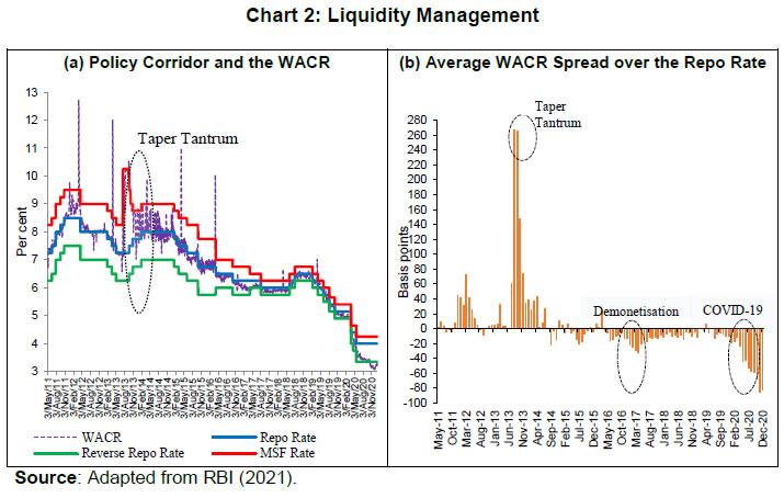 During the period mid-2011 to end-2020, the liquidity management operations of the RBI have faced stiff challenges on three occasions. First, when liquidity was tightened by widening the LAF corridor asymmetrically on the upside – increasing the MSF rate to 300 bps above the policy repo rate in mid-July 2013, after global and domestic financial markets were roiled by the “taper tantrum” of May 2013 – coined as the interest rate defence of the exchange rate (Pattanaik and Kavediya, 2015). Tighter daily average cash reserve ratio (CRR) maintenance requirement (at 99 per cent) and restricted access to RBI liquidity reflected in significant tightening of the WACR, which subsequently eased with the withdrawal of exceptional measures (Chart 2 (a)). Second, the liquidity glut post-demonetisation, which prompted the RBI to impose an unprecedented incremental CRR of 100 per cent, temporarily, for one fortnight (RBI, 2017a). The liquidity overhang imparted a softening bias to overnight rates, reflected in the persistence of a large negative spread of the WACR vis-à-vis the repo rate (average of about 19 bps) over a year after demonetisation (Chart 2 (b)).14 Third, the unprecedented level of liquidity injection through various conventional and unconventional measures since February 2020, particularly after the outbreak of COVID-19 coupled with large capital inflows resulted in a liquidity glut with the WACR trading below the repo rate by 50 bps (on an average) during February-December 2020.15 In contrast, the WACR traded below the repo rate by 10 bps (on an average) during June 2019-January 2020, when the stance of monetary policy was changed from neutral to accommodative in June, 2019. III.2 Salient Features16 III.2 (a) Policy Corridor At its inception in May 2011, the LAF corridor was symmetric with a width of 200 bps and it continued to be so till mid-July, 2013. Consequent to the havoc wrought by the taper tantrum on domestic financial markets, the Reserve Bank asymmetrically widened the corridor to 400 bps in mid-July 2013 (Chart 3 (a)).17 With the return of normalcy, the corridor width was gradually restored to its pre-crisis level by end-October, 2013. Thus, the LAF corridor remained symmetric for a major part since its commencement. Subsequently, the corridor width was tapered from 200 bps to 100 bps in April, 2016 and further to 50 bps in April, 2017, in response to the liquidity glut post-demonetisation (RBI, 2021). Following the financial market dislocations after the outbreak of the pandemic, the corridor width was asymmetrically widened downwards to 90 bps in two stages (Chart 3 (b)). 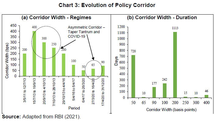 The optimal width of the corridor and its impact on liquidity management has been extensively debated in the literature (Bindsel, 2014). Specifically, a wider corridor is associated with (i) higher interbank turnover; (ii) smaller central bank balance sheet size; and (iii) higher short-term interest rate volatility.18 A wider corridor is symptomatic of tight monetary policy where central bank liquidity is costly for banks; hence, lower average recourse to standing facilities spur interbank trading activity. Empirical research suggests that the width of the corridor is positively associated with volatility in the inter-bank market – a wider corridor is symptomatic of higher volatility and vice versa (Bindseil and Jablecki, 2011). With markets stabilising after the taper tantrum, the progressive narrowing of the corridor moderated volatility – measured by the exponential weighted moving average (EWMA)19 of the WACR – significantly, corroborating the cross-country experience (Chart 4). Such moderation, however, did not have any significant adverse impact on the share of the call money market in total money market turnover and it continued to remain below 10 per cent.20 Despite the widening of the corridor, there is no perceptible change in volatility after the outbreak of COVID-19.  III.2 (b) Reserve Maintenance and Averaging Under Section 42(2) of the Reserve Bank of India Act, 1934, banks are required to maintain a fraction of their NDTL as CRR balances with the Reserve Bank on an average daily basis over a reporting fortnight with a stipulated minimum daily maintenance.21 Changes in the monetary policy framework and refinements in the operating procedure over time has gradually de-emphasised the CRR – from 6 per cent of NDTL in May 2011 to 3 per cent by March 2020, but raised thereafter in phases to 4.5 per cent by May 2022. Although the efficacy of the CRR is limited in a modern financial system,22 minimum reserve requirements have helped in guiding and stabilising overnight rates. In a reserve averaging system, commercial banks’ daily reserve holdings cannot fall below a stipulated level which helps in complying with the overall requirements for the entire maintenance cycle (Hamilton, 1996). In fact, banks’ demand for reserves are elastic on a daily basis, but interest inelastic on a longer-term basis due to the mechanism of reserve averaging and the presence of standing facilities (Patra et al., 2016). In India, the daily minimum reserve requirement was prescribed to provide greater flexibility to banks in optimising their reserve holdings, based on their cash flows during the fortnight. Within the reporting fortnight, banks flexibly optimise their daily maintenance levels based on interest rate expectations vis-à-vis the rates on standing facilities (Chart 5 (a)). The daily minimum reserve requirement was enhanced from 70 per cent of NDTL (effective since December, 2002) to 99 per cent in July, 2013 but subsequently, it reduced to 90 per cent by April 2016. After the outbreak of the COVID-19 pandemic, it was lowered to 80 per cent in March, 2020 in view of hardships faced by banks due to social distancing of staff and consequent strains on reporting requirements. Subsequently, it was reverted to 90 per cent by September, 2020. If the daily minimum requirement is very high, it constrains the flexibility of banks during the reserve maintenance period. For instance, the intra-fortnightly variation (across the weeks) in reserve maintenance was negligible when the daily minimum was prescribed at 99 per cent after the taper tantrum as compared with significant frontloading of reserve maintenance in the first week vis-à-vis the second week when daily minimum balance was set at 70 per cent (Chart 5 (b)).  IV.1 Data The empirical exercise involves daily data from May 9, 201123 to December 31, 2020 spanning 2332 observations. The data is sourced from (i) Reserve Bank of India; (ii) Bloomberg; and (iii) Thomson Reuters. The variables included in the empirical exercise, rationale for their inclusion and expected impact on the WACR spread are discussed below. IV.1 (a) List of Variables – Theoretical Predictions As discussed in Section II, banks are prone to unanticipated liquidity shocks – particularly, towards the end of the business hours in a day. Hence perforce, they must take recourse to the standing facilities. In fact, these unforeseen liquidity shocks have the maximum impact on the overnight rate and, consequently, the spread. As deliberated in the preceding sections, the interplay of demand and supply factors in the uncollateralised overnight money market determines the WACR spread. Since the demand and supply factors are intertwined and reflected only in the final outcome (WACR), we identify these factors (variables) from key features of the Indian overnight money market, such as (i) liquidity drivers; (ii) market microstructure; (iii) interest rate expectations; (iv) operating procedure; and (v) risk measures based on the existing literature (Linzert and Schmidt, 2011; Kucuk et al., 2016; Nath, 2015; and Kumar et al., 2017). The set of explanatory variables are: (i) Liquidity Conditions: The Reserve Bank injects discretionary liquidity through (i) the LAF window; (ii) outright open market operations (OMOs); and (iii) refinance provided to banks.24 Whereas outright OMOs are usually undertaken to provide durable/ enduring liquidity, LAF operations are targeted to address transient/ frictional liquidity mismatches in the system. As such, changes in autonomous drivers of liquidity (viz., currency in circulation, forex operations and government cash balances) are stabilised through countervailing policy actions (viz., changes in open market operations – both outright and reversible repurchase transactions – and CRR, occasionally). During systemic liquidity stress, banks with adequate collateral can avail liquidity from the Reserve Bank; thus, increasing net liquidity injections through the LAF. On the contrary, easy liquidity conditions results in lower recourse to liquidity from the Reserve Bank. Thus, the quantum of funds availed under the LAF is symptomatic of systemic liquidity conditions.25 For the empirical exercise, we define liquidity conditions as the net LAF position on any day as a proportion of the average daily CRR requirement, following the literature (Linzert and Schmidt, 2011; and Kucuk et al., 2016).26 Under deficit liquidity conditions, increase (decline) in this ratio on any given day would signify liquidity tightness (easing), reflected in firming up (softening) of the WACR spread. (ii) Liquidity Distribution: Based on the revised liquidity framework implemented in September 2014, a major portion of the assured liquidity from the Reserve Bank was available through variable rate term repo auctions. From a theoretical perspective, it would imply that a few banks can potentially avail all liquidity auctioned through term repos, provided (i) they have the required collateral; and (ii) they can bid aggressively in the auctions (Linzert and Schmidt, 2011). While these few banks are the beneficiaries of the auction, there may exist many banks who are short of funds but do not have adequate collateral backing to access central bank liquidity. The deficit banks, inevitably, may seek funds in the unsecured market, while banks having surplus funds can lend at exorbitantly high rates based on their counterparty (borrower) risk assessment. In fact, the beneficiary banks can arbitrage by lending at a premium in the inter-bank market with funds borrowed from the central bank.27 Thus, even if systemic liquidity requirements are fully met by a central bank, the skewed distribution of liquidity across banks may encourage arbitrage opportunities which may result in the hardening of WACR and widening of the spread. In this study, liquidity distribution is captured by the ratio of inter-bank unsecured (call) money market volume as a proportion of total volume (both unsecured and collateralised segment) in the overnight money market. Illustratively, a skewed distribution of liquidity (few participants bidding successfully at the central bank liquidity auctions) is likely to result in higher dependence on the call money market from a systemic perspective. Therefore, an increase in demand for call money relative to the total overnight money market volume would exert pressure on the WACR, thereby increasing the spread.28 (iii) Liquidity Uncertainty: The uncertainty about funding liquidity can also have an impact on overnight interest rates. Before September 2014, the unlimited liquidity accommodation available under the LAF had largely eliminated this element of uncertainty which returned after the imposition of limits on borrowing. These borrowings from the LAF window were made available through variable rate term repo auctions. As a result, banks became unsure about the amount of liquidity that could be procured through auctions, given the uncertainty about bidding by other market players in the auction. Consequently, banks may bid aggressively both in term repo and in the overnight market to garner all available liquidity which would put overnight rates under stress. From the literature (Linzert and Schmidt, 2011), we capture liquidity (funding) uncertainty with the conditional volatility from cumulative reserve maintenance during a reporting fortnight as it reflects the uncertainty about banks demand for liquidity and their bidding behaviour in auctions (Linzert and Schmidt, 2011). (iv) Expectations and Uncertainty on Interest Rates: Expectations on short-term interest rates also determine intra-maintenance period demand for liquidity. Since banks try to minimise the cost of maintaining required reserves, their current demand for liquidity increases (decreases) if the overnight rates are expected to harden (soften) in the remaining days of the maintenance cycle and vice versa. We take the difference of the 14-day MIBOR29 from the policy repo rate to capture interest rate expectations within the reserve maintenance cycle. Widening of this spread implies that short-term rates are likely to increase in the later part of the maintenance period; therefore, banks would demand more funds presently to frontload maintenance. For determining the medium-term outlook on interest rates, banks keenly follow the central bank’s statements and actions on the future course of monetary policy. Therefore, expectations about future policy rate movements, particularly close to the policy announcement dates, play a key role. Overnight indexed swaps are commonly used by financial institutions for interest risk management with the floating leg of the swap linked to the MIBOR. By design, OIS contracts act as a futures segment for the money market which is useful in extracting the “surprise” component of any “news” impact on money market rates.30 Since all expected information is priced into the OIS rates, it is only sensitive to unexpected market news. The OIS rate moves in anticipation of upcoming monetary policy decisions well before the actual policy is announced; therefore, we take the 1-month overnight index swap (OIS) rates as our measure of near-term market expectation about the policy rate.31 It is argued that demand for bank reserves are positively related to policy expectations, i.e., firming up of the OIS rate results in higher demand for funds which, in turn, will reflect in a hardening of the WACR and its spread (Beirne, 2012 and Lloyd, 2021). We also introduce a variable capturing the uncertainty about interest rates. As discussed above, uncertainty about the direction/quantum of monetary policy rate adjustments can render the interest rate outlook uncertain over the medium term. An uncertain outlook, in turn, can impart considerable volatility to demand and, consequently, to the WACR spread. Therefore, we use the conditional volatility of the 14-day MIBOR rate to capture the interest rate uncertainty over a fortnight. (v) Lagged Spread: The theory suggests that if market frictions are absent, today’s expected level of interest rates for tomorrow should be equal to that of tomorrow’s interest rate [i.e,. it − Et(it + 1) = 0]; otherwise inter-temporal arbitrage possibilities exist.32 Since the interbank overnight market is characterised by volatility clustering,33 lagged spread indicating persistence may also be positively related to the WACR spread. (vi) Dummy Variables: We define four dummy variables capturing some key features of (i) the operating procedure; (ii) unprecedented monetary policy actions; (iii) institutional features of the Indian financial system; and (iv) an event that played a key role in influencing the spread, particularly during some specific periods. The four dummies are: (a) Corridor Width Dummy: As discussed in the preceding section, the width of the corridor has an impact on volatility and spread. Since the corridor width was 200 bps for a major part of the sample period, we have taken a corridor width of 200 bps to define alternate regimes. Thus, while -1 defines the WACR for being below the reverse repo rate, 1 characterises the WACR for being above the MSF rate as compared with 0 being within the corridor. (b) Quarterly Dummy: In the Indian financial set up, quarterly tax payments drain liquidity from banks. As a result, banks’ do not lend but build up cash balances mainly for managing their balance sheet which results in liquidity shortage in the overnight market, leading to spike in overnight interest rates at the quarter-end. We capture this phenomenon with a quarterly dummy which takes the value 1 for each quarter-end date (0 otherwise). (c) Structural Liquidity Dummy: As discussed before, the liquidity management framework underwent several changes in response to the taper tantrum. These changes, particularly the hike in the minimum daily CRR requirement to 99 per cent of the required reserves in July 2013, reduced flexibility of banks and increased their demand for overnight liquidity thus exerting pressure on spreads. Most of these changes were, however, reversed by end-October 2013. This phase has been captured by introducing a structural liquidity dummy with value 1 for each day of the period July 17 to October 28, 2013 and 0 for other days. (d) Demonetisation Dummy: High value currency notes of ₹1000 and ₹500 denominations worth ₹15.4 lakh crores – constituting more than 86 per cent of the erstwhile total currency in circulation in the economy – was demonetised on November 8, 2016 (RBI, 2017b). These notes were deposited in banks which resulted in a liquidity glut in the interbank market plummeting the WACR below the reverse repo rate. This phenomenon continued till April 2017 when the negative spread of the WACR over the reverse repo rate peaked at 32 bps but moderated thereafter to an average of about 15 bps over the next seven months. In view of this, we define a demonetisation dummy which takes the value 1 from November 9, 2016 to April 30, 2017 and 0 otherwise. To summarise, the variables along with its expected impact on spread are listed and presented below (Table 2). IV.2 Methodology IV.2 (a) Multinomial Logit Model34 Multinomial logit model is used in economic analysis to explain variation in an unordered categorical dependent variable with more than two levels as a function of one or more independent variables. In the context of this paper, the multinomial logit model helps in predicting the behaviour of the call rate under different regimes, given the set of independent variables. The multinomial logistic equation with categorical dependent variable Y with 1, …., J levels and independent variables of X1, …., Xp can be modelled as the probability of each level j of Y by  where, β is the parameter of regressors of dimension k and b is the vector of parameters to be estimated by maximum likelihood estimation. The sign of the βj tells us whether the change in Xi will make the jth (j = -1,1) regime more / less likely relative to the within regime (j = 0). One of the limitations is that the βj parameter does not depend on the level of Xi or other variables in the model (Long and Freeze, 2014). Exponentiating the βj parameter helps us to interpret the results in terms of odds ratio. The odds ratio provides the increase or decrease in the odds of being in the jth (j = -1, 1) regime compared to the reference within regime (j = 0) when the explanatory variable is increased by a unit, keeping all other variables constant. The odds ratio, however, does not indicate the magnitude of the change in the probability of the outcome. The marginal effect analysis (Long and Freeze, 2014) provides a better understanding of the model as it measures the change in the probability of an outcome (j = -1,1) relative to the reference category (j = 0) for a change in the Xi, keeping all other independent variables at specific values. For the continuous explanatory variable, the marginal effect computes the effect of an infinitely small change in Xi while the marginal effect computes the effect of discrete change in Xi for the discrete case. In this study, we report the average marginal effects by calculating each individual observation’s marginal effect and then take the mean. IV.3 Empirical Results In our model, the call money spread is categorised under three regimes:  This study explores the factors responsible for the call money rate lying in the two extreme regimes using the multinomial logit model. To provide identification to the multinomial logit model as also to get the probability of being in extreme regimes, we set Yj=0 as the base reference category. In our sample, most of the total observations (94.8 per cent) were within regime, while around, 3.9 per cent and 1.3 per cent were in the low and high regime, respectively (Table 3).
Some descriptive statistics of the explanatory variables are presented in Table 4. The variables are not normally distributed, as evident from Skewness and Kurtosis. The mean and standard deviation of the variables must be different in each regime to support the existence of three regimes, as mentioned above. The preliminary findings support the categorisation of data into three regimes (Table 5). The Table presents the average values of the independent variables when the WACR is within the MSF and Reverse Repo rate (within regime” - column 2); the WACR being lower than the Reverse Repo Rate (“low regime” - Column 3); and being higher than the MSF rate (“high regime” - Column 4). Comparison of “within regime” and “low regime” suggests that the overnight market behaves differently during the “within regime” as compared to the “low regime”, as p-value of t-test (indicating equality of means) are significant (Table 5: Column 5). In a similar manner, the probability of equality of means test comparing “within regime” and “high regime” are also highly significant (Table 5: Column 6). The comparison of equality of means for all three regimes are tested simultaneously through the one-way analysis of variance (ANOVA) test and are also found to be significantly different across regimes (Table 5: Column 7)35. Given the evidence of the three regimes being different, it provides the rationale for the use of the multinomial logit model. Section IV.1(a) describes the explanatory variables considered for the econometric exercise. Inclusion of all the explanatory variables in the multinomial logit model may lead to drastic increase in the number of parameters to be estimated. In this scenario, the maximum likelihood estimates tend to deteriorate quickly while model interpretation suffers (Tutz et al., 2015). To identify the explanatory variables that explains the regime choice in the multinomial logit model, the least absolute shrinkage and selection operator (LASSO) technique is used (Simon et al., 2013; and Vincent and Hansen, 2014; 2019)36. The LASSO penalty not only improves the model fit but it also conducts automated feature selection37. In the LASSO technique for the multinomial logistic regression model, the coefficients are chosen to minimise the multinomial log-likelihood plus a penalty term that penalises the size of the model through the sum of absolute values of coefficients. The LASSO technique for multinomial logit model can be represented as  where, ℓ is the multinomial log-likelihood, y is the outcome variable, x is the vector of the dependent variables; λ coefficient determines the amount of shrinkage in the lasso regression and ‖β‖2 is a grouped-lasso penalty on all the K coefficients for a variable, which makes them all zero or non-zero together. To select the optimal λ coefficient, we used the cross-validation technique, which aims to condition the variable selection process on the out-of-sample prediction than the in-sample model fit.38 First, all the continuous variables in the dataset are standardised so that the LASSO technique can accurately compare the importance of each variable.39 The penalty factor λ coefficient is chosen such that the area under the curve (AUC) measures are maximised for the testing data. Using this technique, the final explanatory variable selected for our analysis are liquidity condition, within period spread, liquidity distribution, policy expectation, interest rate uncertainty, liquidity uncertainty, quarterly dummy, structural liquidity dummy and corridor width dummy. The estimated results of the parameters of the multinomial logit model and the corresponding odds ratio for the high and low regimes compared to the within regime are reported in Table 6. The log-likelihood ratio test for the fitted model is significant, indicating that the current model using explanatory variables provided a better fit than the null model with no explanatory variables in predicting the logit of being in either low or high regime compared with the within regime. The positive coefficients of the multinomial logit model indicate that the probability of observing high or low regime increases compared to within regime as the value of the explanatory variable increases, whereas negative coefficient indicates reduction in probability of observing high or low regime compared to within regime. In a similar vein, odds ratio of greater than one indicates the increase in odds of observing high or low regime compared to within regime, while less than one odds ratio indicates the reduction in odds of observing high or low regime compared to within regime when Xi increases. As shown in the upper part of Table 6, the within period spread and policy expectation reduced the probability of observing low regime compared to within regime and are highly significant. Increase in within period spread results in market participants expecting the WACR to firm up above the repo rate, i.e., either in the “within regime” or “high regime” rather than at the low regime. In a similar manner, if the policy expectation increases, i.e., the 1-month OIS rate is higher than the repo rate, market players expect the WACR to firm up above the repo rate, thereby increasing the observations in either “within regime” or “high regime” as compared to “low regime”. Increase in expectations of liquidity uncertainty increased the probability of observing low regime compared to within regime and are highly significant. This may be attributed to expectations of market participants that the RBI may overcompensate in terms of liquidity injections to address market concerns about rising overnight money market interest rates from aggressive bidding. The lower part of Table 6 indicates that liquidity conditions, within period spread, policy expectation, quarterly dummy, structural liquidity dummy, and corridor width dummy influenced the probability of observing high regime compared to within regime. Increase in liquidity condition, within period spread, quarterly dummy, structural liquidity dummy, and corridor width dummy increased the probability of observing high regime compared to within regime, while increase in policy expectation decreased the probability of observing high regime compared to within regime. Under deficit liquidity conditions, the increase in the liquidity conditions ratio signify tight liquidity, reflected in firming up of the WACR above the MSF rate, thereby increasing the probability of observing high regime. As expected, increase in within period spread, quarterly dummy and structural liquidity dummy increased the probability of observing high regime compared to within regime. The corridor width dummy lower than 100 basis points also increased the probability of observing high regime compared to within regime. This is not surprising given that an increase (reduction) in corridor width implies tight (easy) monetary policy. As such, any liquidity forecasting error in a narrow corridor could lead to the call money rate breaching the corridor ceiling (above the MSF), thereby increasing the probability of being in the high regime. The increase in policy expectation decreases the probability of observing higher regime compared to with-in regime. As explained in the methodology above, we use the average marginal effects (AMEs) for interpreting the model, which is the most useful summary statistics of the effects (Long and Freeze, 2014). Table 7 presents the average marginal effects of change in the probability of observing low, within and high regimes for a change in the explanatory variables. The continuous variables viz., liquidity conditions, within period spread, liquidity distribution, policy expectation, interest rate uncertainty and liquidity uncertainty are increased by one standard deviation, while all the dummy variables are characterised by discrete changes (from 0 to 1).40 The average marginal effect shows that an increase of one standard deviation in within period spread (around 55 basis points) is associated with the statistically significant 0.03 reduction in the probability of identifying the call money rate in the low regime. This is offset by an increase of 0.02 (weakly significant) in the probability of identifying the call money rate as high regime. The results suggest that higher the spread of the 14-day MIBOR rate over the repo rate, the probability of call money spread being in high regime is higher; hence, effective liquidity management warrants continuous monitoring of intra-period spread. The average marginal effect for policy expectation shows that one standard deviation increase in policy expectation (around 54 basis points) is associated with the reduction in probability (0.024) of identifying the call money rate as low regime. This result is expected as increase in policy expectation will lead to market participants anticipating a tighter monetary policy leading to higher WACR. In a similar manner, an increase in policy expectation leads to the call money rate being within spread regime by a probability of 0.02 and decrease in the probability of being in high regime by 0.006. These results can be explained by market expectation of the RBI managing liquidity conditions to keep the WACR range bound within the corridor. The average marginal effect for liquidity uncertainty shows that one standard deviation increase in liquidity uncertainty (about 3.7 times) is related with the significant 0.029 increase in probability of identifying the call money rate as low regime. This is offset by a significant decrease of 0.031 in the probability of identifying the call money spread as within regime. The results suggest that whenever liquidity forecasts for the present period are not accurate, resulting in increased liquidity uncertainty, market participants expect that the RBI may overcompensate in the next period. The predicted probability of identifying the call money spread as high regime is on average 0.09 higher on the quarter-end days. This result is mainly due to banks’ unwillingness to lend surplus amount due to capital provisioning considerations, thereby constricting the inter-bank market volume leading to call money rate breaching the upper end of the policy corridor. IV.4 Robustness In our sample, the observance of low regime and high regime are rare events compared to within regime. The empirical literature has shown that occurrence of rare events even with large samples may have substantial bias, as maximum likelihood estimation of logistic model suffers from small sample bias (King and Zeng, 2001).41 Using Monte Carlo simulation of logistic regression, Leitgöb (2020) concluded that penalised maximum likelihood estimation (Firth, 1993) is the best model for estimating rare events42. Given the above, we re-estimated our multinomial logit model with penalised maximum likelihood method (Kosmidis and Firth, 2011; and Kosimidis, 2020) as a robustness check (Table 8). The estimates of our model are similar to that of the multinomial logit model using maximum likelihood method in terms of sign and significance, only the magnitude of the coefficients is marginally different. This indicates that our results are robust even after accounting for the presence of rare events in the model. As a further check on the robustness of the findings, the model was augmented with a Post-COVID Dummy which includes a set of dates representing large accretion to systemic liquidity through the conduct of long-term repo operations (LTROs) and targeted long-term repo operations (TLTROs) during February-March 2020.43 A priori, the Post-COVID Dummy will have negative impact on call money spreads as huge amount of policy-induced liquidity injections reduce banks’ reliance on the inter-bank market thereby moderating market activity which, in turn, reduces the call money spread. The multinomial logit model was re-estimated by including the Post-COVID Dummy in the base baseline model (Table 9). The results are broadly similar to Table 6 – in terms of sign and significance albeit with some changes in the magnitude of the coefficients, thus validating our baseline findings. This paper attempts to delineate the impact of institutional features and market microstructure on movements in the operating target of monetary policy, using machine learning tools and daily data on the Indian overnight money market spanning nearly a decade. While there is a vast literature analysing the overnight and policy rate spread, this study concentrates on the institutional, seasonal, structural and idiosyncratic factors at play along with the central bank liquidity operations in identifying the key determinants of the inter-bank rate relative to the policy interest rate corridor. Specifically, we focus on the factors that would cause the interbank rate to breach the corridor in either direction using the multinomial logit model. Using the LASSO technique, the explanatory variables that are found to be important are liquidity conditions, within period spread, liquidity distribution, policy rate expectations, interest rate uncertainty, liquidity uncertainty, quarterly dummy, structural liquidity dummy and corridor width dummy. From the empirical exercise, it transpires that (i) interest rate expectations within the reserve maintenance period; (ii) policy rate expectations; and (iii) liquidity distribution are highly significant in characterising the WACR when it occasionally moved below the reverse repo rate. In contrast, (i) liquidity conditions; (ii) quarterly dummy; (iii) structural liquidity dummy; and (iv) corridor width dummy, besides policy rate expectations and short-term interest rate expectations within the reserve maintenance period turned out to be important when the WACR sporadically breached the MSF rate. The results, reported in terms of average marginal effects, are robust even after accounting for the presence of rare events in the model. Overall, the findings of the paper are useful from the perspective of liquidity management. @ Edwin Prabu A (paedwin@rbi.org.in) is on secondment with Qatar Central Bank, while Indranil Bhattacharyya (ibhattacharya@rbi.org.in) is from the Monetary Policy Department of the Reserve Bank of India. 1 They are grateful to Krishna Mohan Kushwaha, DEPR Study Circle participants and an anonymous external reviewer for comments and suggestions. Data support provided by Bhimappa Talwar and Akshay Gorwadkar is gratefully acknowledged. The views expressed are those of the authors and not of the Reserve Bank of India. 2 Inside lags include (a) recognition of the problem, (b) policy decision to address the problem, and (c) implementation of the decision; while outside lags include (a) immediate impact of the policy decision, and (b) the final outcome (Perryman, 2012). 3 While the MSF provides central bank liquidity to market participants at a premium above the policy rate, the fixed rate overnight reverse repo window allows surplus liquidity to be parked after business hours with the Reserve Bank at a discount below the policy rate. Thus, the standing facility acts as a stabiliser against unanticipated liquidity shocks (RBI, 2014). 4 To control the overnight rate more effectively, the central bank’s model of the overnight rate needs to be comprehensive for precisely identifying the adequate policy measure (Wurtz, 2003). 5 Although central banks can largely influence the supply of liquidity, they are not able to control it perfectly (Moschitz, 2004). 6 The theoretical underpinnings of the interbank market are discussed in Bhattacharyya and Sahoo (2011). 7 Decoding monetary policy intent and actions of the central bank is considered a “signal extraction problem” for market participants because of information asymmetry that exists between them. Central banks often bridge this problem by communicating directly with the market through forward guidance on liquidity conditions; publication of autonomous drivers of liquidity is one such mechanism. 8 The “liquidity effect” represents the ability of the central bank to influence the cost of funds in the economy by changing the price at which it provides liquidity to banks. 9 No bank will lend money at a cheaper rate than what it can get by depositing funds with the central bank; on the other hand, no bank will borrow money at rates higher than the central bank’s lending rate (given it can provide sufficient collateral). Thus, the deposit rate must be lower than the lending rate; otherwise, banks will arbitrage by borrowing at the lending rate and earn the deposit rate by parking funds with the central bank. 10 The flatness depends on the days remaining in the maintenance cycle. Specifically, the demand curve gets steeper on the last day as banks cannot hedge any further and must comply with the overall maintenance requirements (Whitesell, 2006). 11 Monetary policy transmission was found to have a greater and faster impact under deficit liquidity conditions; hence, it was appropriate to operate the banking system in a small deficit under a corridor framework (RBI, 2011). 12 For a discussion on the liquidity impact of forex interventions by the Reserve Bank, see Raj et al., (2018). 13 Some features of the erstwhile liquidity management framework such as (i) the WACR being the operating target; (ii) symmetric corridor having width of 50 bps; and (iii) minimum daily maintenance of 90 per cent of the CRR requirement were retained. For details, see Chapter IV of the Monetary Policy Report, April 2020. 14 Unlike the previous episode, the WACR was relatively stable during the post-demonetisation period. 15 During October-December 2020, the WACR (on an average) dipped below the reverse repo rate by 14 bps on account of heavy capital inflows. 16 Analysis is based on 2332 observations spanning the period May 2011 to December 2020, excluding holidays and week-ends. 17 An asymmetric corridor has been proposed for an ailing economy and a frail financial sector (Goodhart, 2010). In practice, it has gained wider acceptability among many advanced economy central banks, notably the ECB, after the global financial crisis. 18 In contrast, zero corridor width – central bank lending and accepting deposits at the same rate – would throttle the overnight market and bloat up the central bank’s balance sheet (Tucker, 2004). In this scenario, reviving the overnight market would require imposing restrictions on central bank lending/deposit facilities (Bindseil and Wurtz, 2008). 19 As a volatility measure, the EWMA is an improvement over simple variance as it assigns greater weight to more recent observations. Thus, EWMA expresses volatility as a weighted average of past volatility where the weights are higher for more recent observations. 20 After the declaration of the Covid-19 pandemic in March 2020, market activity shifted from unsecured to secured markets (Dilip, 2021). 21 The averaging for reserve maintenance is also allowed in the ECB, the US Fed and many other jurisdictions. While the ECB does not prescribe any daily minimum requirement, the Fed’s reserve averaging is subject to a specified criterion. 22 Reserve requirements is a blunt instrument to fine tune the money supply (Mishkin, 1997), moreover, it is difficult to change reserve requirements frequently. 23 Week following the implementation of the new monetary policy operating procedure effective May 3, 2011. 24 The Expert Committee (RBI, 2014) argued for discontinuing with all sector-specific liquidity facilities; accordingly, export credit refinance was withdrawn in February 2015. In the wake of COVID-19, refinance was reintroduced for select all India financial institutions (AIFIs) to address liquidity stress in specific sectors. 25 The extent of liquidity support would determine the impact on overnight rates, i.e., if the Reserve Bank fully offsets the ex-ante liquidity mismatch, overnight rates would be completely stable. 26 Since the average daily requirement is constant over the maintenance period, it is more of a scale factor. The daily net LAF position, therefore, determines the direction of the ratio. 27 Given the counterparty (credit risk) risk of the borrowers. 28 A more homogenous distribution of central bank liquidity would largely satisfy the liquidity requirement of each bank thereby reducing their dependence on the inter-bank call money market; consequently, pressures would ease on the WACR and the spread. The positive relationship between the ratio and WACR spread reflects the lack of depth in the call money market where few players often drive market dynamics (Kumar et al., 2017). 29 Mumbai Interbank Outright Rate – the rate at which funds are availed by banks from the interbank market. 30 The no-arbitrage condition ensures that the fixed leg of an OIS contract should be equal to the expected overnight rates compounded daily for the period of contract, plus a term premium. Therefore, if overnight rates are expected to firm up (soften) during the period of contract, the OIS rate should consequently increase (reduce). 31 One month to one-year US OIS rates are generally used as measures of US interest rate expectations (Lloyd, 2018). 32 For a discussion on the martingale properties of overnight interest rates in the context of the US, see Hamilton (1996). 33 Refers to episodes of volatility in which "large changes tend to be followed by large changes, of either sign, and small changes tend to be followed by small changes” (Mandelbrot, 1963). This resulted in the development of GARCH models whose main intuition is that asset volatility tends to revert to some mean rather than being constant or moving monotonically. 34 For a detailed discussion, see Greene (2012). 35 Equality of means for two regimes can be done by t-test; however, comparison of equality of means for more than two regimes can be done appropriately by the ANOVA test. 36 We have estimated using “tidymodels package using the underlying “glmnet” package”, R package. 37 LASSO techniques are increasingly used in econometrics for model selection and variable selection.An overview of machine learning techniques in applied econometrics is given by Mullainathan and Spies (2017). Belloni et al., (2014) present a rigorous introduction on the use of LASSO for inferring from high-dimensional data while Asis et al., (2020) uses LASSO for variable selection. 38 In our analysis, we used 10-fold cross-validation technique with 70 per cent of the data as training data and 30 per cent as testing data. Further, we used stratification on the 3 regimes to ensure that we have representation of all the three regimes in both training and testing data. 39 Since the data set has class imbalance (or rare events), that is 3.9 per cent and 1.3 of the data are in high and low regimes, we used the data augmentation for the minority class using the Synthetic Minority Oversampling Technique (SMOTE) in the training dataset, such that the minority classes will have approximately half as many observations as the majority classes. 40 Most of the earlier studies found liquidity conditions to be significant as a major part of their sample period were characterised by deficit liquidity conditions. In contrast, liquidity conditions are not found to be significant in this study as a large part of the sample period was characterised by surplus liquidity because of demonetisation and the COVID-19 pandemic-induced large liquidity injections. 41 See also Paul Allison “https://statisticalhorizons.com/logistic-regression-for-rare-events”. 42 See also Richard William website “https://www3.nd.edu/~rwilliam/stats3/RareEvents.pdf”. 43 These dates are: February 17, March 02, March 09, March 18, March 27, April 03, April 09, April 17, and April 23 of 2020. References Asis, G., Chari, A., & Haas, A. (2020). Emerging Markets at Risk. AEA Papers and Proceedings. 110, 493-98. Bech, M. & Monnet, C. (2013). The Impact of Unconventional Monetary Policies on the Overnight Interbank Market. Reserve Bank of Australia Conference Volume. Beirne, J. (2012). The EONIA Spread Before and During the Crisis of 2007–2009: The Role of Liquidity and Credit Risk. Journal of International Money and Finance. 31(3), 534-551. Belloni, A., Chernozhukov, V., & Hansen, C. (2014). Inference on Treatment Effects after Selection among High-Dimensional Controls. The Review of Economic Studies, 81(2(287)), 608-650. Bernhardsen, T., & Kloster, A. (2010). Liquidity management system: Floor or corridor. Norges Bank Staff Memo No 4 Bhattacharyya, I. & Sahoo, S. (2011). Comparative Statics of Central Bank Liquidity Management: Some Insights. Economics Research International. Bindseil, U. (2000). Central bank liquidity management: theory and euro area practice. available at< http://www.ecb.int/events/pdf/conferences/1b.pdf>. Bindseil, U. (2014). Monetary policy operations and the financial system. Oxford University Press. Bindseil, U. & Jablecki, J. (2011). The Optimal Width of the Central Bank Standing Facilities Corridor and Banks' Day-to- Day Liquidity Management. ECB working paper No. 1350. Bindseil, U. & Würtz, F. R. (2008). Efficient and Universal Frameworks (EUF) for Monetary Policy Implementation mimeo, European Central Bank. Cassola, N. & Morana, C. (2008). Modeling Short-Term Interest Rate Spreads in the Euro Money Market. International Journal of Central Banking. 4(4), 1-37.Dilip, A. (2021). Changing Tides in the Indian Money Market. RBI Bulletin. November. Firth, D. (1993). Bias reduction of maximum likelihood estimates. Biometrika 80(1),27–38. Forbes, K. J., & Warnock, F. E. (2012). Capital flow waves: Surges, stops, flight, and retrenchment. Journal of International Economics. 88(2), 235-251. Ghosh, S., & Bhattacharyya, I. (2009). Spread, volatility and monetary policy: Empirical evidence from the Indian overnight money market. Macroeconomics and Finance in Emerging Market Economies. 2(2), 257–277. Goodhart, C (2010). Liquidity management in Financial Stability and Macroeconomic Policy, a symposium sponsored by the Federal Reserve Bank of Kansas City, 157-168. Greene, W.H. (2012). Econometric Analysis. 7th edition. Prentice Hall. Hassler, U. & Nautz, D. (2008). On the Persistence of the Eonia Spread. Economics Letters 101(3), 184-187. Hamilton, J. (1996). The daily Market for Federal Funds. Journal of Political Economy, 104(1), 26-56. Kavediya, R. & Pattanaik, S. (2018). Operating Target Volatility: Its Implications for Monetary Policy Transmission. Reserve Bank of India Occasional Papers 37 (, No. 1&2). King, G. & Zeng, L. (2001). Logistic Regression in Rare Events Data, Political Analysis 9, 137-163. Kosmidis I (2020). brglm2: Bias Reduction in Generalized Linear Models. R package version 0.6.2. Kosmidis, I, & Firth, D. (2011). Multinomial logit bias reduction via the Poisson log-linear model. Biometrika 98(3), 755–759. Küçük, H.; Özlü, P., Talaslı, A. Ünalmış, D. & Yüksel, C (2016). Interest Rate Corridor, Liquidity Management, And The Overnight Spread, Contemporary Economic Policy, Western Economic Association International, 34(4), 746-761. Kumar, S., Prakash, A., & Kushawaha, K. M. (2017). What explains call money rate spread in India? RBI Working Paper Series: 07/2017. Leitgöb, H. (2020). The Problem of Modeling Rare Events in ML-based Logistic Regression: Assessing Potential Remedies via MC Simulations. Accessed from https://www.europeansurveyresearch.org/conf/uploads/494/678/167/PresentationLeitg_b.pdf Lloyd, S. P. (2018). Overnight index swap market-based measures of monetary policy expectations. Bank of England, Staff Working Paper No. 709. Lloyd, S.P. (2021). Overnight indexed swap-implied interest rate expectations. Finance Research Letters. 38 (January), 1-8. Linzert, T. & Schmidt, S. (2011). What explains the spread between the Euro overnight rate and the ECB's policy rate? International Journal of Finance & Economics, 16(3), 275-289. Long, J.S. & Freese, J. (2014). Regression Models for Categorical Dependent Variables Using Stata, Third Edition. College Station, TX: Stata Press. Mandelbrot, B. B. (1963). The Variation of Certain Speculative Prices. The Journal of Business, 36(4), 394-419. Mishkin, F. S. (1997). The Economics of Money, Banking and Financial Markets, Fifth edition, Addison-Wesley, Massachusetts, Boston. Moschitz, J. (2004). The Determinants of the Overnight Interest rate in the Euro Area. European Central Bank Working Paper Series No. 393. Mullainathan, S. & Spiess, J. (2017). Machine Learning: An Applied Econometric Approach. Journal of Economic Perspectives, 31 (2), 87-106. Nath, G.C. (2015). Repo market – A tool to manage liquidity in financial institutions. Macroeconomics and Finance in Emerging Market Economies, 8(3), 286–305. Neyer, U. 7 Wiemers, J. (2004). The Influence of a Heterogeneous Banking Sector on the Interbank Market Rate in the Euro Area. Swiss Journal of Economics and Statistics (SJES). 140(3), 395-428. Patra, M.D. & Kapur, M. (2012). A Monetary Policy Model for India. Macroeconomics and Finance in Emerging Market Economies. 5(1), 16-39. Patra M.D., Kapur M., Kavediya R., & Lokare, S.M. (2016). Liquidity Management and Monetary Policy: From Corridor Play to Marksmanship in Ghate C.& Kletzer K. (eds) Monetary Policy in India, Springer, New Delhi, 257-296. Perryman M.R. (2012). The Measurement of Monetary Policy. Springer. Pattanaik, S. & Kavediya, R. (2015). Taper Talk and the Rupee–Preconditions for the Success of an Interest Rate Defence of the Exchange Rate. Prajnan, 44(3), 251-277. Raj, J., Pattanaik, S., Bhattacharyya, I. & Abhilasha (2018). Forex Market Operations and Liquidity Management, RBI Bulletin, August. Reserve Bank of India (2011). Report of the Working Group on Operating Procedure of Monetary Policy (Chairman: Deepak Mohanty), March. -------------, (2014). Report of the expert committee to revise and strengthen the monetary policy framework (Chairman: Dr. Urjit Patel), January. -------------, (2017a). Annual Report 2016-17, August 30. -------------, (2017b). Macroeconomic Impact of Demonetisation - A Preliminary Assessment. March. -------------, (2019). Report of the Internal Working Group to Review the Liquidity Management Framework, September. -------------, (2020). Statement on Developmental and Regulatory Policies, February 6. Schaechter, A. (2001). Implementation of monetary policy and the central bank’s balance sheet. International Monetary Fund Working Paper No. 149. Simon, N, Friedman, J., & Hastie, T. (2013). A Blockwise Descent Algorithm for Group Penalized Multiresponse and Multinomial Regression. https://web.stanford.edu/~hastie/Papers/multi_response.pdf. Singh, B. (2020). Liquidity Shocks and Overnight Interest Rates in Emerging Markets: Evidence from GARCH Models for India. RBI Working Paper Series, WPS(DEPR):06/2020. Soares, C., & Rodrigues, P.M.M. (2011). Determinants of the Eonia Spread and the Financial Crisis. Working Papers, 12/2011. Banco de Portugal. Tucker, P. (2004). Managing the Central Bank’s Balance Sheet: Where Monetary Policy Meets Financial Stability. Bank of England Quarterly Bulletin, Autumn, 359-382. Tutz G, Pößnecker W, & Uhlmann L (2015). Variable selection in general multinomial logit models. Computational Statistics & Data Analysis, 82, 207-222. Valimaki, T. (2006). Why the Marginal MRO Rate Exceeds the ECB Policy Rate. Bank of Finland Research Discussion Papers 20, 2006. Vincent M, Hansen, N.R. (2014). Sparse group lasso and high dimensional multinomial classification. Computational Statistics & Data Analysis. 71, 771–786. Vincent, M. and Hansen, N. R. (2019). msgl: Multinomial sparse group lasso. R package version 2.3.9. Whitesell, W. (2006). Interest Rate Corridors and Reserves. Journal of Monetary Economics.53, 1177-1195. Wurtz, F. R. (2003). A Comprehensive Model of the Euro Overnight Rate. ECB Working Paper 207. | |||||||||||||||||||||||||||||

ଏହି ପେଜ୍ ଶେୟାର୍ କରନ୍ତୁ:


ରିଜର୍ଭ ବ୍ୟାଙ୍କ ଅଫ୍ ଇଣ୍ଡିଆ ମୋବାଇଲ୍ ଆପ୍ଲିକେସନ୍ ଇନଷ୍ଟଲ୍ କରନ୍ତୁ ଏବଂ ଲାଟେଷ୍ଟ ନିଉଜ୍ କୁ ଶୀଘ୍ର ଆକ୍ସେସ୍ ପାଆନ୍ତୁ!
ଆମର ଆପ୍ ଇନଷ୍ଟଲ୍ କରିବାକୁ QR କୋଡ୍ ସ୍କାନ୍ କରନ୍ତୁ


ପେଜ୍ ଅନ୍ତିମ ଅପଡେଟ୍ ହୋଇଛି:


