 IST,
IST,


RBI WPS (DEPR): 08/2014: A Financial Conditions Index for India
| RBI Working Paper Series No. 08 1Financial market variables contain information about the future state of the economy. Changes in financial variables often translate into changes in the real economy. Very often financial variables send contradictory signals to economic agents. Further, acute information asymmetry exists in financial markets especially around trigger events during times of crises. Breaking information asymmetry assumes importance since lack of timely and correct information further perpetuates uncertainty and deepens the crisis. To overcome the problem of information asymmetry, financial condition indices (FCI) are constructed. Given this backdrop, this paper constructs a financial conditions index for India using monthly data between January 2004 and August 2013. Variables from the money, bond, foreign exchange and the stock markets have been combined in a Principal Components Framework to form the aggregate financial conditions index. The aggregate FCI is the synthesis of information from all the markets. Prima facie, it appears that this FCI also has reasonably high correlation with growth in IIP and GDP. JEL Classification Number: C43, E44, E52, G14 Keywords: Financial Conditions Indices, Principal Components I. Introduction Changes in financial market variables have long been believed to affect the real economy. Economic agents often alter their expectations about economic activity and hence their behavior in response to movement in financial variables. Over the decades there have been tremendous developments in financial markets. Newer financial products have been invented, cutting edge technology has been increasingly used in financial markets, transaction costs have fallen, innovations in product design have been implemented and financial markets around the world are more integrated today than ever before. All this has given rise to meteoric increase in financial activity around the world. The increase in the number of financial products has meant that there are more variables to account for in economic estimates/expectations today than in the past. The problem is not only that of many variables to monitor but also conflicting signals sent by market variables about financial conditions. Illustratively, with the onset of the financial crisis in mid - 2007, there was a general re-pricing of risk in the OECD financial markets (Guichard and Turner, 2008). The initial damaging effects of the crisis were felt when equity prices fell, yields on corporate bonds increased, Credit Default Swaps (CDS) spreads of corporates and banks widened and credit standards in general tightened. Governments and central banks, on the other hand, responded to this initial shock by pursuing expansionary fiscal policies and cutting interest rates/postponing interest rate hikes. While the first set of changes in financial variables point towards tight financial situation, the second set of changes are indicative of accommodative financial state. Conflicting indications like these often present economic agents with the problem of correctly assessing the financial conditions prevailing in the economy. Against this backdrop it is natural to ask whether stock prices should be monitored or CDS spreads or policy interest rates or all of these variables simultaneously to assess financial conditions? Is it possible to identify the common information set in financial variables by constructing an index? Can information content in financial variables be used to assess financial conditions and perhaps the future state of economic activity? The present paper seeks to address some of these questions in the Indian context using monthly data between January 2004 and August 2013. This research paper is organised as follows, section - II traces literature on financial conditions and financial conditions indices, section - III deals with variable selection, the methodology and index construction. Section – IV discusses the movement in the financial conditions indices. Section V concludes the paper. What are Financial Conditions? The need for correct and timely information for smooth functioning of financial markets can hardly be over emphasised. Lack of information perpetuates uncertainty which disrupts market functioning. Systemic dimension of information uncertainty was not realised early by market participants during the global financial crisis (Oet et al., 2012). Many financial crises are triggered by specific events such as bank failure or sovereign default. However, the build-up to such a crisis is not always readily visible. Conditions in financial markets, i.e. financial conditions, are not directly observable; changes in financial conditions often manifest themselves inmovement in market variables. It may be useful to think of financial conditions as a latent unobservable variable, a change in which is depicted by change in the observable financial market variables. Thus, changes in market variables must necessarily indicate a change in financial conditions. For instance, increasing spreads could depict tightening financial conditions. Bernanke (1990) explores the possible explanations of the super-ordinate information content in the commercial paper (CP) - Treasury bill (T-bill) spread. Since the CP and T-bills have the same maturity profile, the spread between the two measures the risk of default or credit risk (assuming very little liquidity risk) associated with the issuer of CP. Now, if the market expects economic conditions to worsen in the future, then the perception of risk of default associated with issuers of CP increases and hence the yield on CPs is bid up in order to make CPs attractive enough to be held by the market. Therefore, in general, a high CP-T-bill spread is indicative of worsening future economic conditions. In the extreme case, rapidly deteriorating financial conditions are often characterised by rapidly increasing risk premia, high spreads and falling asset prices. Further, stress in one segment of the financial market can be transmitted to the other segments due to the integrated nature of modern day financial markets. The extent of transmission is, obviously, a moot point. However, it is also possible that stress in one market is neutralised by favourable conditions in some other market. Thus, assessing financial conditions as whole becomes difficult. This problem is often overcome by synthesising information for all relevant markets and combining movement in financial variables into an index. This sort of index is usually called the Financial Conditions Index (FCI). In essence, any FCI is the synthesis of various, sometimes contradictory, signals from financial markets. Why is tracking of Financial Conditions necessary? Information asymmetry in context of overall conditions prevailing in financial markets often deepens a crisis and it also influences market behaviour which, during times of crises, is characterised by fire sales or fall in activity. Thus, breaking information asymmetry in this context assumes great importance. A financial conditions index can serve as a tool to break the information asymmetry regarding the state of overall financial conditions. Changes in financial variables, often, lead to changes in real economic activity. Further, monetary policy affects the real economy by changing the relative price/value of financial assets. This in turn alters the behaviour of agents and brings about real economic change. A considerable volume of literature exists on channels of monetary transmission. A sound understanding of the various channels of transmission is necessary to analyze the effects of policy changes on different segments of the financial markets and the consequent changes on economic variables. Boivin et al. (2009) have classified the modern channel of monetary policy transmission into two parts, viz., first, the neo classical channel and second, the non neo classical channel. The neo classical channel encompasses the investment channel which studies the effect of long term interest rates on the cost of capital and the effect of asset price changes on the demand of new physical capital. In addition, the consumption channel (wealth and inter-temporal substitution effect) and the trade based channels (impact of real exchange rates on net exports) also constitute the neo classical channel of monetary transmission. The non neo classical channel of monetary transmission comprises of effects of imperfections in credit supply and balance sheet constraints of borrowers. Therefore, it may be possible to gauge the effect of policy changes on financial conditions and economic variables. However, the effect of policy changes can vary from variable to variable and may sometimes transmit signals which are unclear. It may hence be prudent to combine relevant variables to study the effect of policy changes on financial conditions which translate in to changes in economic activity. For instance, Stock and Watson (1989) found that the spread between commercial paper rates (CP) and Treasury bill rate (T-bill), 10-year government bond and 1-year government bond, housing starts, manufacturer’s unfulfilled orders in durable goods industries and growth of part time work are good predictors of business cycles. The results in Stock and Watson (1989) indicated that a low commercial paper-treasury bill spread, high 10-year government bond-1-year government spread, high unfulfilled orders and rise in housing starts were indications of strong economic performance of the economy in the future. It is also found that stock markets often affect the economic variables in the economy via the wealth effect and the confidence channel and play an important role in transmission of monetary policy impulses. Cassola and Morana (2002) find that stock markets and relative assets prices in general play an important role in monetary transmission. The dynamic nature of market microstructure also makes it imperative to understand the dynamics of the change on economic activity. It is possible that, when not taken into account, the correlation of changes in monetary policy to financial conditions could bias the impact of monetary policy changes on economic activity (Swiston, 2008). Thus, the study of financial conditions in the conduct of monetary policy assumes importance in this context. However, studying movements in different financial assets in isolation may be of limited use as each variable contains information only about a certain aspect of the economy and does not say anything about the other aspects. This problem can be overcome by constructing an index from all relevant financial variables to capture all the information in one statistic. FCI is said to summarize information about the future state of the economy contained in current financial variables (Hatzius et al., 2010). Select Financial Conditions Indices around the World In addition to assessing the current state of financial conditions; financial conditions indices have also been used as lead indicators of economic activity. Although numerous FCIs have been constructed in the past, only a few are under discussion here. It is widely believed that the Bank of Canada pioneered the construction of an index capturing information content in financial variables. Strictly speaking, Bank of Canada’s index was a Monetary Conditions Index (MCI) which included variables used traditionally to explain monetary transmission, i.e. interest rate and exchange rate. The weights on the variables were determined by a macroeconomic model constructed to study the effect of change in interest rate and exchange rate on GDP. More formally, the MCI was a combination of the 90-day commercial paper rate and the multilateral exchange rate with a weight of one-third on the exchange rate. This MCI was used as the operational target of policy in Canada (Freedman, 1995). More recently, Illing and Liu (2003) and Gauthier et al. (2004) constructed financial conditions index for Canada using different methodologies. Illing and Liu (2003) combine variables from the banking sector, foreign exchange, equity and debt markets using weights from factor analysis, credit weights and variance equal weights. Gauthier et al. (2004) also use three methodologies to assign weights i.e.an IS-Curve based model, a generalized impulse response function and factor analysis. Results in Gauthier et al. (2004) suggest that in addition to the traditional variables of the MCI (interest rate and exchange rate), housing prices, equity prices and bond yield risk premiums are significant in explaining output during 1980-2000. Perhaps one of the earliest FCIs to be used by investment banks was the Goldman Sachs Financial Conditions Index (GSFCI). The GSFCI consists of the 3-month Libor, A - rated corporate bond yield, trade weighted index and the market capitalisation of all US equities relative to GDP (Dudley, 1999). The weights on the variables are derived from the Federal Reserve’s macro model for the US economy. However, the weight on the stock market variable was increased from what was been indicated by the macro model. One per cent increase in the index represents 100 basis points increase in short term and long term rates, one per cent increase in the trade weighted dollar index and one per cent decrease in the stock market capitalisation to GDP ratio. Macroeconomic Adviser’s Monetary and Financial Conditions Index (MAFCI) studies the contribution of interest rates (short term and long term), equity cost of capital, exchange rate, wealth effect of consumer spending and residential investment on GDP (MA, 2003). The effect of each of these variables on GDP was estimated from Macroeconomic Adviser’s (MA) econometric model for the US economy. MA’s FCI was able to foretell the collapse during the dot com bubble burst. Another frequently tracked financial conditions index is the Bloomberg financial conditions index (BBFCI). It is used to keep track of the strain in the US financial markets. Spreads in the US money market and bond market along with measures of equity prices and volatility are used to assess the stress in the US financial markets (Rosenberg, 2009). The BBFCI is an equally weighted index with the each market receiving one-third weight. Variables in each market receive a weight of 1/n, where n is the number of variables selected from the market. In its original form, the BBFCI did not capture sectoral asset prices bubbles therefore variables capturing asset price bubbles and deviation of interest rates from long term mean were included since late 2009.The newer BBFCI showed considerable stress in the US financial market in the period just before the Lehman Crisis which the original BBFCI failed to capture. Interest in tracking financial conditions appears to have increased after the global financial crisis as evidenced by a spurt in the literature on these indices. A large amount of economic literature has been dedicated to understanding whether information content of financial variables could have been used to predict the global financial crisis. Swiston (2008) uses a VAR framework and impulse response functions to construct a FCI for the US. Looking to explore the impact of availability of credit via the credit channel of monetary transmission, the Federal Reserve’s Senior Loan Officer Opinion Survey on Lending Practices is used to proxy for the availability of credit. Along with this survey results, this FCI includes seven other variables i.e. 3-month Libor, yield on investment grade corporate bonds, GDP, GDP deflator, oil prices, equity returns and real effective exchange rate. The Libor is preferred over the Federal funds rate because it (was believed to) is able to capture the effect on changes in economy wide financial conditions and not just the monetary policy change. Non-bank credit is also tied to the Libor, so the Libor better captures the rates prevailing in the market. The Libor also contains the market’s expectation of monetary policy rates. To proxy for long term interest rates, the yield on investment grade corporate bonds with 5-10 years residual maturity is used. This includes the long term risk free rate as well as the default premia for corporates. A two lag VAR is used to estimate the FCI. The major finding in Swiston (2008) is that over 20 per cent of contribution of financial factors to growth comes from availability of credit. In particular, a 20 percentage points net tightening in lending standard reduces GDP by 0.75 per cent over a one year horizon. Another index tracking financial conditions is the OECD FCI constructed by Guichard and Turner (2008). The FCI included measures of real short term interest rate, real long term interest rates, high yield bond spread, credit standard tightening, real exchange rate and stock market capitalisation. The relative effects of these variables on GDP were used to derive the weights on each variable. The weights are then normalised such that a one per cent increase in the index has the same effect of a one percentage point (100 basis points) increase in the real long term interest rates. The inclusion of a survey measure of tightness in non-price credit banks lending standards in the form of the Federal Loan Officers Opinion Survey is a novelty in this paper (Swiston, 2008 also uses this survey). Reduced form equations and unrestricted VAR framework was used to derive weights. The OECD FCI suggested that from the onset of the crisis in late 2008 financial conditions in the US witnessed considerable stress even with easing monetary policy and a falling dollar. Guichard and Turner (2008) found that that tightening in non-price credit tightening had large effects on GDP which was similar to the effect of a 280 basis points increase in long term real interest rates. In response to the global financial crisis, the US Federal Reserve undertook unprecedented support measures to prop up the US economy which included special lending programs. However, cognizant of the fact that an early exit from there measures in times of high financial stress could jeopardise economic recovery, the Federal Reserve of Kansas City constructed a Financial Stress Index (KCFSI) in 2009 to measure the financial stress in the US economy. Five factors contributing to financial stress were identified. These include i) increased uncertainty about fundamental value of assets, ii) increased uncertainty about behaviour of other investors, iii) increased information asymmetry, iv) decreased willingness to hold risky assets and v) decreased willingness to hold illiquid assets (Hakkio and Keeton, 2009). To capture these aspects of financial stress eleven financial variables were selected viz, i) 3-month Libor and 3-month T-bill spread, ii) 2-year swap spread, iii) of-the-run/on-the-run 10 –year treasury spread, iv) AAA rated corporate bond spread and 10-year treasury spread, v) BAA and AAA rated corporate bond spread, vi) high-yield bond and Baa rated corporate bond spread, vii) consumer ABS and 5-year treasury spread, viii) negative correlation between stock and treasury returns, ix) implied volatility of stock prices x) idiosyncratic volatility of bank stock prices, xi) cross section dispersion of bank stock returns. These variables are combined in a principal components framework such that the coefficients on the variables explain the maximum movement of the variables. The KCFSI showed high levels of financial stress during times of crisis from 1991 onwards. In line with the strand of literature which deals with effects of changes in financial conditions on growth Beaton et al. (2009) construct a FCI for the US which accounts for changes in growth due to changes in financial conditions and is also able to capture stress in financial conditions. In essence, Beaton et al. (2009) construct two FCIs, one using structural vector error correction model (SVECM) and the other using large scale macro-economic model. The large scale macro model includes factors that influence investment and consumption. These are i) federal funds rate, ii) conventional mortgage rate, iii) business borrowing rate , iv) Real Effective Exchange Rate (REER), v) financial wealth, and iv) lending standard for consumer spending, mortgages and business investment. In the SVECM, the commercial paper rate, the business borrowing spread, loan standards for consumer spending and financial wealth. Response of GDP growth rate to structural shocks associated with each variable is used to calculate the FCIs. Beaton et al. (2009) modelled the FCI such that one unit increase in the index has the same impact on GDP as a 100 basis points increase in short term interest rate. Financial wealth, lending standards and short term interest rates play an important role in explaining the FCI. ECB (2009) constructs a global index of financial turbulence (GIFT) for 29 major economies which captures stress in the fixed income, equity and foreign exchange markets using term spread variables in the fixed income market, monthly stock returns and time-varying volatility in stock returns in the equity markets and volatility in the foreign exchange market. The St. Louis Federal Reserve’s Financial Stress Index (STLFSI) is based on 18 financial markets variables which include interest rates, yield spreads, volatility index among other variables (Kliesen and Smith, 2010). The weights on these variables are derived from principal components. Louzis and Vouldis (2011) use market and balance-sheet data to construct a financial systemic stress index for Greece. Variables from the banking sector, equity, money and fixed income markets are used in a principal component framework to arrive at the index. Matheson (2011) used dynamic factor model (DFM) to construct FCI for the USA and the Euro Area so that data can be used even when there are publication gaps. A broad range of variables have been used. The primary finding of this study is that not only is the FCI a useful summary measure of financial conditions, it is also contains useful information about the future of the economy. Hollo et al. (2012) construct a Composite Indicator of Systemic Stress (CISS) for the Euro Area using portfolio theory to aggregate five market sub-indices. Apart from data on financial market variables, data on financial market intermediaries and financial market infrastructure is also used. Another recent addition to this literature is the Financial Stress Index of the Cleveland Federal Reserve. This index uses 16 variables over six market segments i.e. funding, foreign exchange, credit, equity, real estate and securitisation markets using dynamic weighting method (Oet et al. 2012). Published literature studying aggregate monetary or financial conditions in India is scarce. Kannan et al. (2006) use the conventional variables (interest rate and exchange rate) to construct a MCI for India. Weights on these variables are derived from aggregate demand equations using output growth as the dependent variable. The call rate and the 36-country trade based REER are used in the MCI. Once the weights have been derived, the MCI is derived as the weighted sum of deviations of interest rate and exchange from the base period (Kannan et al., 2006). The weight on interest rate is 0.58 and that in exchange is 0.42. Another specification of the MCI also uses bank credit as an additional variable. The paper finds that the MCI is more aligned to GDP growth than to inflation. More recently, Mishra et al. (2012) construct a systemic liquidity index (SLI) for India using spread variables in financial markets in a variance-equal weighing framework. Against the backdrop of the relatively scare literature on Indian financial conditions indices, in this paper we attempt to construct a financial conditions index for India. Before starting on the discussion on the actual construction process, understanding the rationale behind using market variables as an indicator of financial conditions is in order once again. Financial conditions can be considered as a latent variable as these conditions are not directly observable. However, changes in financial conditions manifests themselves in the movement of market variables. Thus, changes in market variables must necessarily indicate a change in financial conditions. We exploit this nature of market variables to construct a financial conditions index. III. Selection of Variables, Methodology and Index Construction It is possible to include any financial market variable in the construction of a FCI as every financial market variable contains some information. However, it is impractical to include every financial variable. Literature on FCI serves as an important guide in identifying variables which could be included in the FCI for India. Financial markets in India can broadly be classified into four segment namely i) money market, ii) bond market which comprises of the government bond market and the corporate bond market, iii) foreign exchange market and iv) equity market. Each market plays a significant role in the economy and changes in these markets also affect economic variables. Broadly speaking, all these markets also play a role in monetary transmission in some way or the other.2 The next section discusses the rationale behind inclusion of variables in the FCI. Data are monthly and pertain to the 116 month period between January 2004 and August 2013. Money Market Variables: A number of central banks all over the world operationalise monetary policy via the overnight money market. Thus, in some sense the call rate is the most important rate in the money market. Even in India, the call rate is the operating target of monetary policy. Changes in the policy rate have an impact on the call rates. The transmission of policy rate changes is strongest and has almost an immediate effect on call rates (RBI, 2011 and Ray and Prabu, 2013). Call rates in turn determine the cost of overnight funds for banks and hence influences the cost of credit for individuals and corporates. Call rates in India move with the policy rate. Therefore, an increase in call rates on account of increase in policy rates does not necessarily signify stressed/tight financial conditions (also see Mishra et al., 2012). The call rate is found to be around the policy rate during “normal times” and further above the policy rates during stressed times. Hence, we define a variable “call spread” as the difference between the weighted average call rate and the effective policy rate. The higher call rates are from the policy rates, financial conditions would be that much more stressed. Before May 2011, during times of liquidity surplus the reverse repo was the effective policy rate and during times of liquidity deficit, the repo rate was the effective policy rate.3 Therefore, effective policy rate is defined as, Effective Policy Rate = Repo Rate if Net LAF > 0 (Injection)
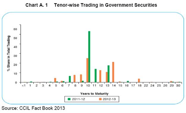
Therefore, the spread of the call rate over the effective policy rate captures stress in the call market. Higher cost of credit on account of higher spread, ceteris paribus, lowers investments and hence affects output negatively. Analogously to the call spread, two other variables “CBLO spread” (CBLO Rate minus the effective policy rate) and “Market repo spread” (market repo rate minus the effective policy rate) are defined. Banks as well as non-bank entities manage their short term liquidity needs via the CBLO and the market repo segments of the money market. The transaction volumes in these markets are more than that of the call market (See Annexure). Hence, these variables merit inclusion in the FCI. A higher spread signifies relatively stressed conditions. To capture the stress arising out of rising credit risk of the corporate sector at the short end of the interest rate spectrum, the “short spread” is defined as the difference between the 3 month commercial paper yield and the 3 month Treasury bill rate. As already argued in the sections above, rising “short spread” depicts perception of higher credit risk associated with corporates. It contains vital information about the expectations of the market player about the state of the economy in the short term. Hence, a higher spread is associated with tight/stressed financial conditions. Bond Market Variables: Changes in yield on government bonds influence conditions prevailing in financial markets. The rates prevailing on the central government dated securities are considered to be virtually credit risk-free. This yield often serves as a benchmark for interest rate prevailing in the economy. Therefore, any change in these rates leads to changes in price/rates of other financial products. An increase in the rate would make borrowing more expensive for the government as well as other market players. To capture this nature of government bonds, we define “10-year G-Sec” as the yield on the 10 year government bond yields. In the secondary market trading in 10 year government bonds accounts for a high share in total trading in government bonds (See Annexure). Higher borrowing costs affect investment negatively, ceteris paribus. To capture credit risk associated with corporates at the medium and long term we define two variables i.e. i) “5-year spread” as the spread between AAA - rated 5 year corporate bonds and government bond of comparable maturity and ii) “10-year spread” as the spread between AAA - rated corporate bonds and 10 year government securities. We use AAA – rated corporate bonds as about 89 per cent of trading in corporate bonds is accounted for by AAA – rated instruments (Nath, 2012). The government bond and the corporate bond are of the same maturity. Any difference in their yields must, therefore, be due to difference in credit risk and the extent of liquidity. The corporate bonds have a higher yield than the comparable government bond because of a higher risk associated with the private sector vis-à-vis the government. Added to this, the government bonds are more liquid than corporate bonds. If economic conditions are expected to worsen; the spreads increase. A high spread is indicative of tight financial conditions making borrowing more expensive for the private sector. Foreign Exchange Market Variables: To capture conditions in the foreign exchange market we define three variables, i) “Exchange rate” (RBI reference rate with respect to the US dollar), ii) “3 month implied volatility and iii) “Forex CMax” [Forex CMAX = Xt / Max Xj (j = 0, -1,-2,-3 up to 1 year)]. The exchange rate of a currency equilibrates the demand and supply of foreign currency. Stress in the foreign exchange market is often characterised by rapidly deteriorating domestic currency. Changes in other segments of the financial markets have an impact on the value of the rupee. For instance, it is possible that when policy rates are increased, there could be more foreign capital inflows into India to leverage the increased interest rate differential. Alternatively, fall in returns in the domestic stock market could lead to outflow of foreign capital. Generally, the causality between FII inflows and stock market returns runs from stock market returns to FII inflows (Shankar, 2011). Thus, change in the stock market returns could have implications for FII inflows in particular and hence financial conditions in general. “3 month implied volatility” is a measure of the market expected future volatility of the currency exchange rate. Higher values depict more volatility and hence more uncertainty. Stressed financial conditions are characterised by high volatility. “Forex CMax” is described as the ratio of the value of the exchange rate at time t and the maximum value of the exchange rate during the last one year. This ratio is upper bound at one, a value which is witnessed during relatively stressed times. Equity Market: The National Stock Exchange (NSE) accounts for the majority of equity trading in in India. Higher returns attract greater FII inflows which affect valuations and have a positive impact on the overall market sentiment. Initial Public Offers (IPOs) have a greater chance of meeting with success when the secondary markets are performing well. This reduces the cost of capital for corporates. Therefore, conditions in the stock market affect real variables via their effect on the ability of corporates to raise fresh capital at a relatively lower cost, among other factors. In addition, stock markets are said to affect the economy via the wealth and the confidence channel. To capture these aspects of stock market movement we define “NSE returns” as the month-wise year on year return. Further, we define “PE ratio” as the PE ratio of the NSE Nifty. PE ratio is indicative of how much investors are willing to pay per rupee of earnings. Higher values are registered when sentiments about the market are buoyant. In addition, we also define “Stock market capitalisation to GDP Ratio” as the market capitalisation of the NSE to the GDP. Market capitalisation to GDP ratio is said to reflect over valuation or undervaluation of the market. Better market conditions are characterised by relatively high market capitalisation. Data: This paper uses data which are daily averages reported month-wise. Daily data could possibly contain more information but they are also fraught with more noise and idiosyncratic shocks. Hence, to smooth the date daily average for each month between January 2004 and August 2013 is computed. In addition, rates in the money markets firm up at the end of the Indian financial year in March. This is due to, among other factors, the demand for funds by mutual funds who are generally net lenders in the money markets. Hence, March end data for money market variables are dropped as these do not necessarily depict movement pertaining to stress but are driven by market micro-structure considerations. Financial market data by their very nature are prone to extreme fluctuations. Considering that the global financial crisis period lies in between the period of analysis, one would expect considerable fluctuation in our data. Admittedly, the call spread fluctuated in the range - 550 basis points to 511 basis points. Similarly, the exchange rate moved in the range 39.4 – 63.2 during the said period. In addition, the market capitalization to GDP ratio moved in the range of 29.3 – 131.2 (Table 1). Due to the commonality of players in the different segments of financial markets, data are correlated (see Annexure) which allows us to profitably employ Principal Components to derive weights to form the FCI. Methodology The data are such that combining them in level forms could bias the index. Hence, we create z-scores [(xi- μ)/σ] for each variable. In addition, the data are suitably modified so that higher values reflect tighter financial conditions. Correlation structure and nature of the data prompt us to use principal component analysis (PCA) to derive weights to form the FCI from other competing methodologies. Hakkio and Keeton (2009) and Kliesen and Smith (2010) use principal component to construct the Kansas City Federal Reserve Financial Stress Index and the St. Louis Federal Reserve Financial Stress Index respectively. Relationship between many independent variables can be examined using the PCA. PCA is useful when a large number of variables have to be studied simultaneously. PCA is used to reduce the large number of variables into a linear combination of a smaller set of coherent variables which capture most of the information in the original set of variables. Efficiency gains are realized when the same amount of information is captured using lesser number of variables. Principal components (PCs) are linear combinations of the original variables which accounts for the maximum variation of the original dataset. The first principal component (PC1) accounts for the maximum variation in the original data followed by the PC2 and so on. The derived latent vectors of the PCs are used as weights for the variables to construct the index. For a brief technical discussion see Annexure. For a more detailed discussion see Dunteman (1989). Construction of the Index While it is possible to combine all the variables simultaneously to derive the financial conditions index we prefer constructing FCIs, in a PCA framework, for each segment of the financial markets before combining these FCIs, in a PCA framework, to construct the aggregate FCI. While deriving the weights for each variable, the latent vector of the first principal component is considered. This strategy allows us to track conditions in each segment of the financial market which enables us to isolate market segments which contribute more to aggregate stress. This strategy also enables us to decipher whether financial conditions in one segment are being neutralized by conditions in some other market or not. In sum, the aggregate FCI comprises of four sub-FCIs.
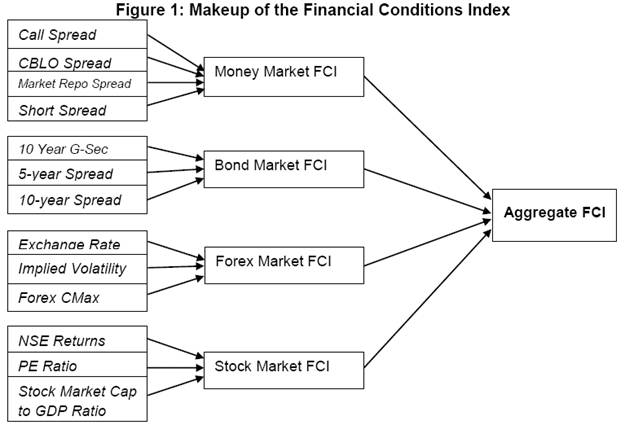
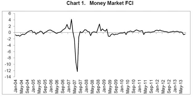
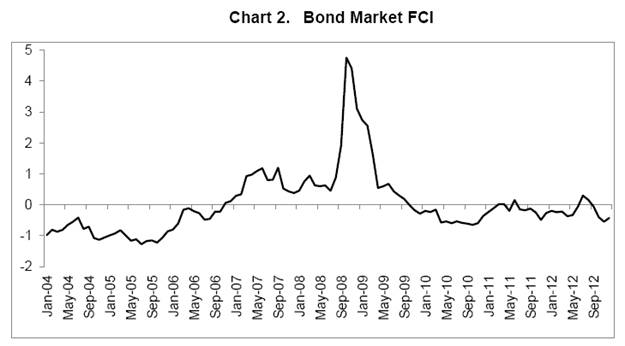
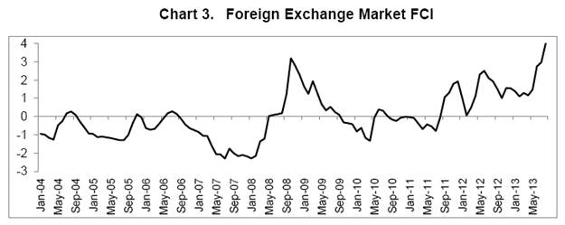
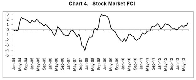
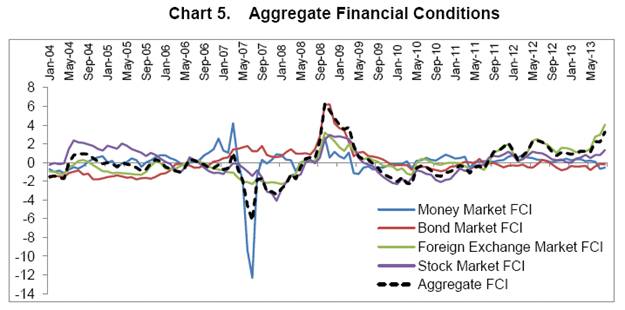
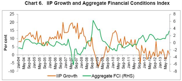
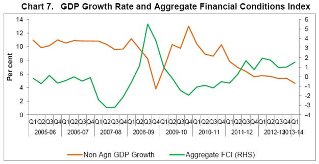
IV. The Financial Conditions Indices: How do they look? Money Market FCI The money market FCI combines information from “Call Spread”, “CBLO Spread”, “Market Repo Spread” and “Short Spread”. The Money Market FCI shows extremely tight conditions in March 2007 (Chart 1). During this period the call rates hardened due to advance tax outflows, credit demand and asymmetric distribution of government securities across banks which could have hindered some banks in accessing the LAF (RBI, 2007). Financial conditions began easing since end May 2007 due to increase in liquidity on the back of government expenditures and foreign exchange operations of the RBI (Ray and Prabu, 2013). The money market rates such as the call rate, CBLO rate and the market repo rate, during June and July 2007, fell below 1 per cent on a number of occasions. The money market FCI shows relatively stressed conditions in October 2008 due to capital outflows from India in connection with the global financial environment (RBI, 2008). During most other time periods under study, the money market FCI has been around the average value. Bond Market FCI The bond market FCI combines information from the “10 year G-Sec”, the “5-year spread” and the “10 - year spread”. Relatively accommodative conditions existed in the bond market from January 2004 till November 2006 (Chart 2). There were signs of increasing stress from July 2008 initially due to increase in government bond yields and then increase in spreads. Extremely stressed conditions existed in the bond market in October 2008 due the global financial crises playing out as well as tight liquidity due to advance tax outflows (RBI, 2008). The stress was also perpetuated by increase in the “5-year spread” and the “10- year spread”. During other periods the bond market FCI is generally around the mean value of zero. Foreign Exchange Market FCI Information from “Exchange Rate”, “3 month Implied volatility”, and “Forex CMax” is summarized in the foreign exchange market FCI. Conditions in the foreign exchange market were relatively benign till May 2008 (Chart 3). This period was characterised by huge capital inflows, relatively stable exchange rate and low volatility. Conditions became very stressed in October 2008 on the evolving aftermath of the Lehman amid high expected volatility and depreciation of the rupee. Downgrade of long term US debt in August 2011 began a general re-pricing of risk in financial markets which resulted in flight to safety and liquidity. In addition, high trade deficit and moderation in capital flows led to a sharp depreciation of the rupee (RBI, 2012). Between February and June 2012, concerns over the stability of the Euro Area led to depreciation of currencies of emerging market economies especially those with large current account deficit. Stress increased further from May 2013 due to a sharply depreciating domestic currency and high volatility as captured by the “3 month implied volatility”. Indication of tapering in the Federal Reserve’s bond purchase programme led to large scale sell off of emerging market assets. Stock Market FCI After being relatively benign during January – April 2004 (Chart 4), conditions in the stock market turned relatively stressed between May 2004 and June 2004 due to uncertainty surrounding the general election results, among other factors, as also the effect of the uncertainty on the PE ratio as well as the market capitalisation. The PE ratio and the market capitalisation fell sharply during May-June 2004. Even though the stock markets witnessed healthy returns during July 2004 and January 2006, the PE ratio and the market capitalisation improved only gradually. Highly accommodative conditions are depicted by the stock market FCI in December 2007 due to high returns, high PE ratio and high market capitalization to GDP ratio. During November 2008, highly stressed conditions existed in the stock markets in the aftermath of Lehman’s bankruptcy. Conditions became benign once again after June 2009 till July 2011. Stress in the stock market reverts to the mean at irregular interval after July 2011. Aggregate FCI Having constructed the FCI for each segment of the financial market, we now focus on combining the sub-FCIs into a composite index to arrive at the aggregate FCI which captures information content in all the markets simultaneously. Principal components are run on the sub-FCIs to arrive at the weights (latent vector of the first principal component) that each market segment commands in the aggregate FCI. The aggregate FCI is a synthesis of the sub-FCIs and takes the following form: Where FCIi is the sub-FCI and wi is the weight derived from the principal component analysis for each sub-FCI5. Movement in interest rates on government securities influences the cost of borrowing for the private sector. Therefore, increase in government bond yield makes borrowing via bonds by the private sector more expensive. Changes in the money market influence the cost of borrowing for banks and other money market players. This in turn influences the rate at which banks lend. Change in interest rate, changes investment and hence output, other factor remaining constant. Changes in the stock market variables influence the economy via the cost of raising resources for the private sector. The sentiment channel also plays an important role. In the forex market, the spot value of the exchange rateas well as the forward implied volatility influence import bill and export receipts as well as capital flows. At each point in time, several factors contribute to the overall financial conditions. In some periods, there could be many opposing pressures on financial conditions. For instance, while the money market variables could depict tight financial conditions, the stock market may depict accommodative financial conditions. Therefore, in sum, the aggregate FCI depicts the net financial conditions taking into account information from all financial markets (Chart 5). From about May 2004 till January 2006 the aggregate FCI is between the sub FCIs providing proof that financial conditions in one market could be off-set by financial conditions in some other market. During this period, relatively more stress existed in the stock market while the other markets witnessed relatively accommodative conditions. Between April 2007 and May 2008, the aggregate financial conditions are relatively benign even though stress existed in the bond market. Unprecedented policy activism in wake of the GFC was witnessed in India between October 2008 and April 2009. The repo rate was reduced by 425 basis points, the reverse repo rate was reduced by 275 basis points and the cash reserve ratio was reduced by a cumulative 400 basis points. In effect, primary liquidity of the tune of 10.5 per cent of GDP was released by these actions (Mohanty, 2009). As a result of the policy measures, the overnight money market rates softened significantly (Misra, 2009). In addition, it is interesting to note that during the July 2008 - December 2008, the yield on government securities also fell. These would perhaps indicate that financial conditions were accommodative. On the other hand, the spread of private sector instruments, viz CPs and corporate bonds increased considerably making the overall conditions relatively tight. From February 2012 onwards aggregate financial conditions have been relatively tight and have been driven to a large extent by stress in the foreign exchange market. The interplay between different markets determines the aggregate financial conditions. This implies that pressures on financial conditions come from different markets at different points in time. Therefore, any policy aimed at correcting the tightness in financial conditions must be cognizant of the source of the tightness. Interpreting the Indices The index depicts stress in an ordinal manner. Hence the difference between two data points in the same series means that stress at one point is lower or higher relative to the other point with the magnitude to difference having little inherent meaning. Since all the FCIs have a mean value of zero, stress could be defined as all values above the mean. Another way to interpret the index would be in relation to its highest or lowest value and assessing how close or far a value is from its extremes. Since the FCIs are based on standardised scores, comparing two indices has no inherent meaning although the direction of movement signifies change in stress. Financial Conditions and Real Economic Activity Accommodative or tight financial conditions must necessarily manifest themselves in changes in the real economy. There is a change in real economic activity whenever there are changes in financial conditions. Thus, any financial conditions index must be able to explain movement in real variables at least to some extent. The general direction of movement of aggregate FCI and rate of growth of IIP is similar (Chart 6). The correlation between the two is about - 0.67 at one period lag. Similarly, the correlation between quarterly nonagricultural GDP growth rate and the quarterly aggregate FCI is - 0.63 (Chart 7).6 This is obviously preliminary evidence which does not establish causality. We do, however, know that periods of high stress are followed by low growth in IIP and GDP. Exploring the causality between FCI and growth in real economic variables forms a fertile ground for further research in this area. This paper seeks to build a robust FCI which captures stress adequately and builds the groundwork for research on the effect of FCI on GDP and IIP growth. As with any index, this FCI should be updated sufficiently often enough so that it is able to capture changes in market microstructure as well as interaction between different financial markets. In addition to this, using quantitative variables such as volume and turnover in financial markets could also be explored. Considerable research has gone into using financial market variables to study stress although stress is not directly observable. However, stress often manifests itself in movement of financial market variables. Stress in one market can be off-set by benign conditions in some other market. Therefore knowing the state of financial condition in an aggregate sense is not always straight forward. Considerable information gaps like these exist in financial markets which in the extreme case leads to breakdown of the market functioning. Thus breaking this information asymmetry assumes importance. To overcome this problem financial conditions indices are constructed which shows the state of financial conditions. In this paper, an ordinal and contemporaneous financial conditions index for India has been constructed. This index is the synthesis of information content in the money, bond, foreign exchange and the stock market. The index shows that tight financial conditions in one market can offset accommodative conditions in some other market thereby making the aggregate conditions tight. Therefore, it is necessary to account for financial conditions in all markets simultaneously in the conduct of policy. Prima facie, the aggregate FCI appears to have some relation with IIP and GDP. However, this research question needs to be explored further to decipher robust relationship between the aggregate FCI, IIP and GDP. @The author is currently a Research Officer (email) in the Financial Stability Unit, Reserve Bank of India. A significant portion of this research was carried out while the author was at the Department of Economic and Policy Research. 1The author would like to thank Shri K.U.B Rao, and Shri Himanshu Joshi and an anonymous referee for their comments and suggestions. The author is also indebted to participants of an internal inter-departmental seminar held at the Department of Economic and Policy Research on May 21, 2013 for valuable suggestions and insights. The author also thanks Dr Partha Ray, Shri G. Jagan Mohan, Shri Gopal Prasad and Shri Edwin Prabu for their insights, comments, and suggestions on an earlier version of this paper. The views expressed in this paper are those of the author and do not represent views of the Reserve Bank of India. 2See Ray and Prabu (2013) for a detailed discussion. 3The Repo rate became the single independently varying policy rate from May 2011 onwards. 4The RBI put in place measures to bring stability in the foreign exchange market in July 2013. The overall allocation of the funds under the Liquidity Adjustment Facility was limited to 0.5 per cent of the net demand and time liabilities of the banking system. This made the MSF rate as the effective policy rate. Also see the Mid-Quarter Monetary Policy statement dated September 20, 2013 (/en/web/rbi/-/press-releases/mid-quarter-monetary-policy-review-september-2013-statement-by-dr.-raghuram-g.-rajan-governor-reserve-bank-of-india-29593). 5As a robustness check, another aggregate FCI was constructed using all variables simultaneously. The correlation between this aggregate FCI with the aggregate FCI reported in the paper was found to be statistically significant at 0.82. 6Quarterly Aggregate FCI is the average of the monthly FCI in the particular quarter. References Beaton, Kimberely., Rene Lalonde., and Corinne Luu (2009), " A Financial Conditions Index for the United States", Bank of Canada Discussion Paper 2009/11, August Bernanke, Ben S (1990), "On the Predictive Power of Interest Rates and Interest Rate Spreads." New England Economic Review" November/December, pp. 51-68 Bernanke. B., (1990): “On the Predictive Power of Interest Rates and Interest Rates Spread”, National Bureau of Economic Research Working Paper No -3486, Cambridge, October. Boivin, J., M. Kiley, and F. Mishkin (2009), “How Has the Monetary Transmission Mechanism Evolved Over Time?” prepared for the third Handbook of Monetary Economics; presented at the Federal Reserve Conference on Key Developments in Monetary Policy, October. Cassola, Nuno and Claudio Morana. (2002), " Monetary Policy and the Stock Market in the Euro Area", European Central Bank Working Paper - 119, January Dudley, William C (1999), "The Goldman Sachs Financial Conditions Index: Still Accommodative After All These Years”, Speech at the Milken Institute Forum on September 20, edited transcript Dunteman, G.H, (1989), "Principal Components Analysis", Sage University Papers, Sage Publications European Central Bank (2009), "Global Index of Financial Turbulence", Box - 1 in Financial Stability Review, December Freedman, Charles (1995), " The Role of Monetary Conditions and the Monetary Conditions Index in the Conduct of Policy", Excerpts from remarks to the Conference on International Developments and the Economic Outlook for Canada, organized by the Policy and Economic Analysis Program, Institute for Policy Analysis, University of Toronto, 15 June Gauthier, Céline., Christopher Graham., and Ying Liu (2004), "Financial Conditions Indixes for Canada.", Bank of Canada Working Paper 2004-22 Guichard, Stephanie, David Turner (2008), " Quantifying the Effect of Financial Conditions on US Activity", OECD Economics Department, Working Paper no 635, September Hakkio, Craig S. and William R. Keeton (2009), " Financial Stress: What Is It, How Can It Be Measured, and Why Does It Matter?", http://www.kansascityfed.org/research/indicatorsdata/kcfsi/ Hatzius. J, P.Hooper, F.Mishkin, K. Schoenholtz and M.Watson., (2010): “Financial Conditions Index: A Fresh Look after the Financial Crisis”, National Bureau of Economic Research Working Paper No -16150, Cambridge, July Hollo, D., M. Kremer., and M.L. Duca (2012), "CISS - A Composite Indicator of Systemic Stress in the Financial System", European Central Bank working paper - 1426, March Illing, Mark and Ying Liu (2003). "An Index of Financial Stress for Canada", Bank of Canada Working Paper - 2003/14, June Kannan, R, Siddhartha Sanyal and Binod Bihari Bhoi (3006), "Monetary Conditions Index for India", Reserve Bank of India Occasional Papers Vol. 27, No. 3, Winter Kliesen, Kevin L. and Douglas C. Smith (2010), "Measuring Financial Market Stress", Federal Reserve Bank of St. Louis National Economic Trends, January Louzis, Dimitrios P and Angelos T. Vouldis (2011), "A Financial Systemic Stress Index for Greece" paper presented at First Conference of the Macro-prudential Research (MaRs) network of the European System of Central Banks, Frankfurt, October Macroeconomic Advisers (2003), A Combined Monetary, Financial, and Fiscal Conditions Index, (An excerpt from the September 19, 2003 issue of Macroeconomic Advisers’ Economic Outlook, December Matheson, Troy (2011), "Financial Conditions Indexes for the United States and Euro Area", Internaitonal Monetary Fund Working Paper - 11/93, April Mishra, Rabi N., G. Jagan Mohan., and Sanjay Singh (2012), "Systemic Liquidity Index for India", Reserve Bank of India Working Paper Series (DEPR) - 10/2012 Misra, BM (2009), "Global Financial Crises and Monetary Policy Response: Experience of India", Breakout Session on Monetary Policy, Regional High-Level Workshop on Strengthening the Response to the Global Financial Crisis in Asia-Pacific: The Role of Monetary, Fiscal and External Debt Policies, Dhaka, July Mohanty, Deepak (2009), "Global Financial Crisis and Monetary Policy Response in India", speech delivered at at the 3rd ICRIER-InWEnt Annual Conference, Delhi, November Nath, G.C (2012), "Indian Corporate Bonds Market-An Analytical Perspective", The Clearing Corporation of India Ltd. Oet, Mikhail V., T. Bianco, D. Gramlich., and S. Ong (2012), " Financial Stress Index: A Lens for Supervising the Financial System", Federal Reserve Bank of Cleveland Working - Paper 12-37, December Ray, Partha and Edwin Prabu (2013), "Financial Development and Monetary Policy Transmission Across Financial Markets: What Do Daily Data tell for India?", Reserve Bank of India Working Paper Series (DEPR) 04/2013, April Reserve Bank of India (2007), "Macroeconomic and Monetary Developments in 2006-07", Mumbai: Reserve Bank of India, April Reserve Bank of India (2008), "Macroeconomic and Monetary Developments - Mid-Term Review 2008-09", Mumbai: Reserve Bank of India, October Reserve Bank of India (2011): Working Group on Monetary Policy Operating Procedures (Chairman: Deepak Mohanty), Mumbai: Reserve Bank of India. Reserve Bank of India (2012), "Macroeconomic and Monetary Developments-Third Quarter Review 2011-12", Mumbai: Reserve Bank of India, January Rosenberg, Michael R (2009), " Financial Conditions Watch: Global Financial Markets Trends and Policy", Bloomberg, September Shankar, Anand (2011), "QE-II and FII inflows into India– Is there a Connection?", Reserve Bank of India Working Paper Series (DEPR) - 19/2011, October Stock, J. and M. Watson, (1989), “New Indexes of Coincident and Leading Economic Indicators,” in Blanchard O. and S. Fischer (eds.), NBER Macroeconomics Annual (Cambridge, MA: MIT), 352-94. Swiston, Andrew (2008), "A U.S. Financial Conditions Index: Putting Credit Where Credit is Due", International Monetary Fund Working Paper - 08/161, June
Principal Components Analysis 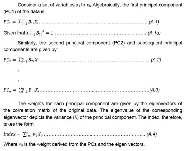
| ||||||||||||||||||||||||||||||||||||||||||||||||||||||||||||||||||||||||||||||||||||||||||||||||||||||||||||||||||||||||||||||||||||||||||||||||||||||||||||||||||||||||||||||||||||||||||||||||||||||||||||||||||||||||||||||||||||||||||||||||||||||||||||||||||||||||||||||||||||||||||||||||||||||||||||||||||||||||||||||||||||||||||||||||||||||||||||||||||||||||||||||||||||||

ଏହି ପେଜ୍ ଶେୟାର୍ କରନ୍ତୁ:


ରିଜର୍ଭ ବ୍ୟାଙ୍କ ଅଫ୍ ଇଣ୍ଡିଆ ମୋବାଇଲ୍ ଆପ୍ଲିକେସନ୍ ଇନଷ୍ଟଲ୍ କରନ୍ତୁ ଏବଂ ଲାଟେଷ୍ଟ ନିଉଜ୍ କୁ ଶୀଘ୍ର ଆକ୍ସେସ୍ ପାଆନ୍ତୁ!
ଆମର ଆପ୍ ଇନଷ୍ଟଲ୍ କରିବାକୁ QR କୋଡ୍ ସ୍କାନ୍ କରନ୍ତୁ


ପେଜ୍ ଅନ୍ତିମ ଅପଡେଟ୍ ହୋଇଛି:


