Press Release

RBI Working Paper Series No. 09
Business Cycles Approach to Dynamic Provisioning: An Indian Case Study
^@Tulasi Gopinath and Thangjam Rajeshwar Singh

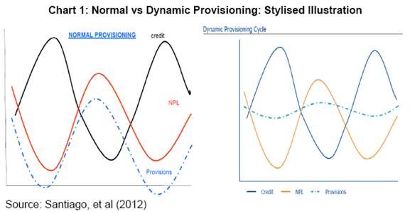
Abstract

There is a broad consensus in the literature that the financial system is procyclical in nature. The procyclicality of the financial system accentuates the phases of booms and busts of the business cycle with severe spillover implications for the real economy. In the wake of the recent global financial crisis, addressing procyclicality of the financial system occupied centre-stage of policy concern for many central banks and financial regulators. This paper attempts to develop a model for rule-based approach to the conduct of dynamic provisioning in India. In India, bank credit of scheduled commercial banks is empirically found to trail the quarterly GDP growth rate during the sample period of 1997 to 2013. Therefore, a model based on GDP growth rate cycle as against the credit cycle could render a better forward looking approach to dynamic provisioning. The rules of dynamic provisioning of the model proposed in this paper are based on real GDP growth rate cycles and the dynamic provisioning is activated when smooth-over-the-cycle GDP growth rate exceeds a certain threshold reflecting the potential output growth. Further, the model also accommodates rules for dynamic provisioning based on inflection points of the business cycle when the economy is in the phase of high economic growth.

JEL Classification: E30, E32, G28

Key Words: Dynamic Provisioning, Potential Growth, Threshold, Activation, Deactivation, State of the Economy, Inflection Point.

Introduction

There is a broad consensus in the literature that the financial system is inherently procyclical on account of variety of reasons: "financial-instability hypothesis (Kindleberger (1978) and Minsky (1982); herd behavior (Rajan 1994; Devenow and Welch 1996); principal-agency problem (Williamson 1963); lack of institutional memory (Berger and Udell (2003)); and financial regulation itself (Saurina and Trucharte (2007); Repullo et al (2009) and Borio et al (2001)). This inherent nature of procyclicality of the financial system has accentuated the phases of booms and busts of the cycle with severe adverse spillover implications for the real economy.

The experience in the context of the recent global financial crisis, in particular, has triggered a debate as to the tools, which could potentially mitigate the procyclical tendencies of the financial system. Capital and provisions are among the broad tools considered for the purpose. Both tools could help to dampen excess credit growth during an expansion. Tool of capital, raises the cost of credit reducing its demand. Tools of provisions, by requiring banks to hold higher provisions, reduces the resources available for funding loans and help restrain credit growth (Gilbert Terrier et al, 2011). In the aftermath of the recent crisis, considerable progress has been made in recommending the capital buffer, a crucial part of Basel III, as a tool to address procyclicality.

On the other hand, dynamic provisioning (DP), as a tool for mitigating procyclicality, has been in vogue even before the crisis. Spanish dynamic provisioning, introduced in 2000, is a case in point. In addition, there have been various approaches to the dynamic provisioning including Uruguayan approach introduced in 2001, Colombian approach in 2007 and Peruvian and Bolivian approaches in 2008. In fact, dynamic provisioning is one of the alternative approaches recommended by the then Financial Stability Forum (2009) for recognizing and measuring loan losses that incorporate a broader range of credit information. The Reserve Bank of India has issued a Discussion Paper on dynamic provisioning in 2012 proposing an Indian variant of the approach to the subject.

Against this backdrop, this paper attempts to showcase a model of dynamic provisioning for India, relying exclusively on business cycles, measured in terms of real GDP¹. Advantages associated with relying in GDP rather than with credit are: it is empirically found that credit trails GDP. Hence, targeting GDP could tend to be more countercyclical than targeting credit. Further, from an EMEs perspective in general and Indian perspective in particular, credit growth per se need not signal emerging financial imbalances due to structural factors.

The rest of the paper is organized into 6 sections. Section II briefly introduces the conceptual underpinnings of dynamic provisioning as an approach, contrast to that of normal provisioning. Section III discusses methodologies adopted in various jurisdictions for the conduct of dynamic provisioning including Spain, Uruguay, Columbia, Bolivia, and Peru. Section IV develops the theoretical model for the conduct of dynamic provisioning in India. Section V estimates the model and showcases the dynamic provisioning rules for India using quarterly GDP data. Section VI back tests the model vis-à-vis the timing of time-varying provisioning requirements introduced in India from time to time since 2004 based on the regulatory judgment. Section VII concludes the paper.

Section II: Concept of Dynamic Provisioning

In this section, attempt is made to understand the concept of dynamic provisioning. Under normal provisioning scenario, provisions are a function of realized losses/incurred losses. In other words, there is a sort of linear relationship between incurred losses and provisions. Provisions rise if losses increase and vice versa. Thus during the boom time characterized by accelerating GDP growth, credit tends to rise. Reflecting all pervasive optimism arising out of favourable business conditions, debtors are able to repay loans promptly. As a result, incurred losses by banks tend to fall and accordingly, provisions tend to fall. On the other hand, during stress times, the opposite happens. GDP growth slows down on the back of deteriorating business environment/confidence. Credit growth decelerates and borrowers find it difficult to repay loans due to which incurred losses by banks mount. Provisions for rising losses, accordingly, increase. Hence, normal provisions are procyclical.

On the other hand, dynamic provisioning framework intends to make provisions a function of expected losses (Mahapatra, 2012) by smoothing provisions along the cycle by advocating a through-the-cycle- approach, as against the point-in- time approach underlying normal provisions. How much smoothening is necessary is a question of choice and judgment. Generally, the objective is to have a stable ratio of provisions to credit over the cycle. The chart below would illustrate the conceptual difference between the normal provisioning and dynamic provisioning.

Section III: Select Country Approaches to Dynamic Provisioning^#

Spain was the first country to put in place a framework for dynamic provisions in 2000. Following Spain, many Latin American countries implemented their approaches to dynamic provisioning (DP). In this section, a brief summary of approaches to DP adopted in Spain, Uruguay, Colombia, Bolivia and Peru is presented.

Spanish Approach

Though Spanish framework was first introduced in 2000, it was modified in 2004. For the purpose of this paper, the modified version is reviewed. The Spanish dynamic provisions formula builds general provisions that account for expected losses in new loans extended in a given period and the difference between average of specific provisions made during the business cycle and the current level of specific provisions. The formula is as follows: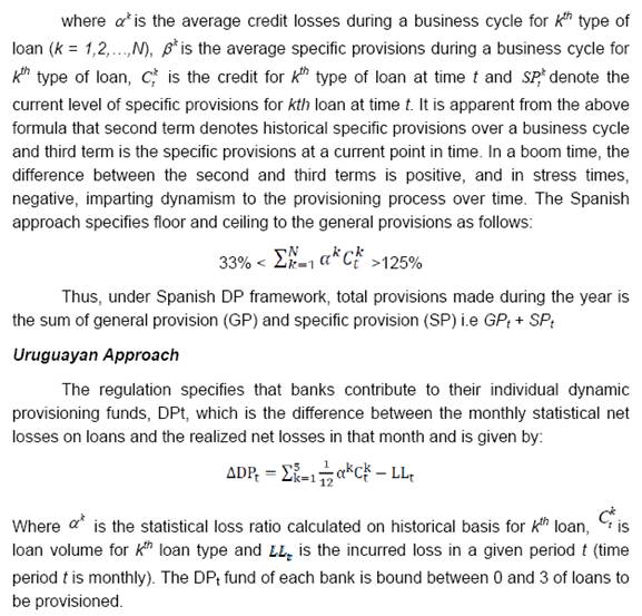

Columbian Approach

Colombia adopted dynamic provisions for commercial and consumer loans in 2007. Banks can measure credit risk of loans using either the regulatory reference model or approved proprietary models. However, at present all banks are using the reference model. The regulatory model prescribes three types of tax-deductable provisions: individual, countercyclical and general provisions. General provisions should at least be equal to 1 per cent of total loans and can be used to meet countercyclical provisions. Countercyclical provisions cover credit risk from changes in the borrower’s creditworthiness due to changes in economic cycle. Countercyclical provisions are treated as special type of specific individual provisions.

The regulator, based on historical data, computes two risk scenarios, matrix A and matrix B, where matrix B is a riskier scenario. Two default probability matrixes of credit type by borrower are generated. Based on expected losses, provisions are calculated as follows:

P = OVL * PD * LGD

Where P is provisions, OVL is outstanding value of loan, PD is probability of default, and LGD is loss given default. Each year, regulators decide which matrix to use to determine the accumulation of individual provisions. During the years of high credit growth, Matrix A is used for calculating individual provisions of each of the banks and the matrix B is used to compute riskier scenario provisions and the countercyclical provisions of each bank is equated to the difference between the individual provisions based on matrix A and the riskier provisions based on matrix B. During stress periods, individual provisions are calculated on the basis of matrix A and there is no accumulation of countercyclical provisions. Further, the accumulated provisions could be drawn down in stress times. Till 2010, there was no objective methodology and the regulator, based on subjective judgment, used to declare “change of status” with regard to the use of the provisions. However, since April 2010, an objective methodology has been put in place to determine the “change of status”. This methodology comprises the following four indicators of deterioration of the portfolio, efficiency, stability, and credit growth. These indicators are defined as follows:

1. Deterioration of the portfolio, based on the variation of individual provisions (P_t)
   ∆ Provisions = (P_t / P_t-3) - 1 ≥ 9%

2. Efficiency: PNR / IC ≥ 17%, where PNR is provisions net of recoveries and IC is interest income

3. Stability: 0 ≤ (PNR / MFBa) ≥ 42%, where PNR is provisions net of recoveries and MFBa is operational margin before depreciation and amortization plus provisions net of recoveries of the credit and leasing portfolio

4. Growth credit portfolio
   ∆CB = (CB_t– CB _t-1) – 1 < 23%, where CB is credit portfolio

The indicators are defined in such a way as to indicate the downturn of the cycle. For each of them, there are precise reference values that trigger the suspension of the accumulation mode. In the default situation, if any of the four indicators is not met, the entity will be subject to accumulation of countercyclical provisions (this will correspond to the cyclical upturn). If the four indicators are met for 3 consecutive months, the entity will enter the depletion phase, where the accumulated provisions are run down (this will correspond to the downturn of the cycle) (Santiago, et al (2012)). Further, when the depletion mode is on, for calculating individual provisions of each bank, while matrix A applied to best credit quality loans, matrix B is applied to lower credit quality loans. Meaning, even in downturn, the provisioning requirements of lower quality loans are relatively stringent.

Bolivian Approach

Banks are required to maintain a dynamic provision in the range of 1.5 per cent to 5.5 per cent of total loans, depending on the type of loan. Banks can access the provision stock to offset upto half of the additional specific provisions required in a given month provided that the loan quality has deteriorated for six consecutive months and the dynamic provision has been fully phased in.

Peruvian Approach

The Peruvian regulators have set a rule based on GDP growth. Under this approach, the countercyclical provisioning rule requires Peruvian banks to build up additional minimum provisions whenever the rule is activated by one of the conditions below:

1. the annualized average percent change of GDP during the past 30 months reaches or exceeds 5 percent from below;

2. the annualized average percent change of GDP during the past 30 months is above 5 percent and the average annualized percent change of GDP during the past 12 months exceeds by 2 percentage points its value one year before;

3. the annualized average percent change of GDP during the past 30 months is above 5 percent and 18 months have elapsed since the rule was deactivated by second deactivation condition.

Countercyclical provisions are deactivated by one of the two conditions below:

1. the annualized average percent change of GDP during the last 30 months falls to or below 5 percent;

2. the annualized average percent change of GDP during the last 12 months is lower by at least 4 percentage points than its value one year before.

As is evident from the select country practices, fundamentally, dynamic provisioning framework is premised on better understanding of the business cycles as it advocates an inter-temporal approach. While majority of the methodologies for dynamic provisioning adopted across jurisdictions rely on banking data involving credit and loss history, there is an alternative methodology using macro-economic data, especially real GDP (Peruvian approach). In the following section, an attempt is made to develop a similar model for India using real GDP data.

Section IV: The Proposed Methodology for Dynamic Provisioning

This section attempts to develop a model of business cycle based approach to dynamic provisioning in India. The conceptual ideas of the proposed model are drawn from the experience of Peruvian model, which is explained in the earlier section.

Burns and Mitchell (1946) defined the classical definition of business cycles as, "Business cycles are a type of fluctuations found in the aggregate economic activity of nations that organize their work mainly in business enterprises: a cycle consist of expansion occurring at about the same time in many economic activities, followed by similarly general recessions, contractions and revivals which merge into the expansion phase of the next cycle; this sequence of changes is recurrent but not periodic. In duration, business cycles vary from more than a year to ten or twelve years; they are not divisible into shorter cycles of similar character with amplitudes approximating their own".

Generally, the widely accepted single data series representing the notion of ‘aggregate economic activity’ of a country is GDP. In the literature, there are basically three different approaches to analyse the business cycle, viz., Classical Cycles, Growth Cycles and Growth Rate Cycles. The Classical business cycle measures the ups and downs in the absolute levels of many economic activities at about the same time in an economy. Growth cycle tracks the upswings and downswings through deviations of the actual growth rate of the economy from its long-run trend of growth. On the other hand, Growth rate cycles are the simple cyclical upswings and downswings in the growth rate of the economic activity, which has become very popular in recent years in the analysis of business cycles. The growth rates are estimated as the simple annual point-to-point growth rates viz., same-month-year-ago, same-quarter-year-ago changes.

Literature on business cycles documents that there are instances wherein classical measure of business cycle could throw out wrong signals in identifying recession of the business cycle phases (Dua and Banerji, 1999). While growth cycle is more suitable for historical analysis, growth rate cycle is more appropriate for real time monitoring and forecasting (Klein, 1998). Therefore, in this paper, growth rate cycle is analyzed. The model formulated in this paper is based on the quarterly real GDP growth rate cycle and the dynamic/cyclical provisioning is activated / deactivated when the rate of growth of real GDP exceeds /falls below a certain threshold level, basically reflecting the potential output growth.

The Model

Suppose, the growth rate cycle of real GDP as measured by same-quarter-year-ago be denoted by g_t, where t = 1, 2, 3… N is the time series. As the estimated growth rate cycles are expected to be quite volatile, smoothing is carried out to eliminate short-term fluctuation in the cycles through the application of moving average method for dating business cycles. But smoothing a series runs a certain risk of distorting the pattern, especially the timing (Zarnowitz et al (2006)). Therefore, in order to reduce the shift in the timing, centered equal weighted moving average method is used for smoothing. For odd period m = 2p+1, for p = 1, 2, 3… P, the centered m-period moving average² of real GDP growth rate cycles, denoted by Y_t is defined as:

The dynamic provisioning is activated/deactivated based on whether the smoothen series of real GDP growth rate over the cycle period T represented by A_t crosses certain threshold of economic growth rate denoted as γ at time t from below or above. Accordingly, the dynamic cyclical provisioning rules, based on the state of the economy, are formulated as follows:

Based on State of the Economy

Rule 1: Cyclical provisioning is activated at time t, when A_t crosses the threshold γ from below i.e. (A_t > γ). The threshold value of λ is empirically estimated.

Rule 2: Cyclical provisioning is deactivated at time t, when A_t crosses the threshold γ from above i.e. (A_t < γ).

Based on the Inflection Point of Business Cycle

Accordingly, the proposed model formulates the following rules for deactivation and reactivation based on the inflection points of the business cycle signifying turnaround in the economic activity as:

Reflecting the principle of conservatism, the model does not propose to suggest any automatic deactivation of dynamic provisions – unlike in the case of reactivation by Rule 5, which is based on the average duration of the phase from trough to peak signifying end of upturn. The iterative procedures involved in the conduct of the proposed model of Dynamic Provisions along with flow chart are presented in Annex-1:A. The next section estimates the theoretical parameters of the model.

Section V: The Model Estimation⁵

To estimate the model, an endeavour is made to understand the characteristics of Indian business cycles. The data on quarterly real GDP (Base Year: 2004-05) covering the period Q1:2004-05 to Q3:2013-14 and quarterly real GDP (Base Year: 1999-2000) covering the period Q1:1996-97 to Q2:2009-10 were taken from the official website of Central Statistics Office (CSO), Government of India. Finally, the quarterly GDP data (Base Year: 2004-05) covering the period Q1: 1996-97 to Q3:2013-14 was obtained by splicing backward. The growth rate cycle is estimated as same-quarter-year-ago change in quarterly real GDP. As the estimated growth rate cycles are volatile, 3-quarter equally weighted centered moving average (Y_t) series is estimated to analyse the business cycle, eliminating the short-term lived volatility in the GDP growth rate⁶. Since the smoothing of the real GDP growth rate would not allow the estimates near the end points, which is required for analysing the recent data for timely policy action, the median forecast of real GDP growth rate (at factor cost) by professional forecasters for the period Q4:2013-14 to Q4:2014-15 were obtained from the quarterly Survey of Professional Forecasters (SPF)⁷ conducted by Reserve Bank of India (RBI) for the quarter October-December 2013 (27th Round), published at RBI website. This would enable the estimates of the smooth series near the end points. The smooth growth rate cycles of real GDP since Q1:1997-98 is presented in Chart 2.

The Characteristics of Indian Business Cycle: Duration and Amplitude of Phases

Central to the understanding of business cycles is to identify its set of turning points, which separate the phases of expansion and contraction. The literature provides what is called Bry and Boschan (1971) business cycle dating algorithm, modified by Harding and Pagan (2002). The Bry and Boschan procedure of dating business cycles for quarterly data is presented in the Annex-1:B. This algorithm detects local maxima (peak) and minima (trough) for a single quarterly series. Between a peak and trough of economic activity, an economy is in a contraction phase (a recession), while between a trough and peak of activity, an economy is in an expansionary phase (a boom). Once the turning points are identified, the characteristics of the business cycle, such as the duration and amplitude of the phases, can be derived, which in turn are used for analysing the dynamic provisioning rules as explained in section IV above. Based on Bry and Boschan algorithm, the identified peak and trough points of the Indian business cycle (Chart 2) since Q1: 1997-98 is presented in Table 1.

The chronology of the Indian business cycles reveals that the average duration of:

• peak to trough (recessionary period) is around 6 quarters

• trough to peak (expansionary period) is around 6 quarters

• the average duration of one business cycle (both peak to peak and trough to trough) is around 11 quarters

The above inference on the average duration and the phases of the cycles is illustrated in the following chart.

Therefore, A_t series which represent the evolution of business cycles over time is obtained by smoothening of the real GDP growth rate over the cycle period, measured by a centered moving average of 11 quarters of real GDP growth rate (g_t) The last five end points of A_t series are estimated based on median forecast of real GDP growth rate by professional forecasters. The evolution of Indian business cycles over time is presented in Chart 4 and Annex-2.

The Threshold γ

Estimation of potential growth rate is vast area of research interest. There are several methodological approaches to the estimation of potential output. Broadly speaking, there are two approaches: the univariate statistical approach and the structural approach. The univariate statistical approach derives estimates based purely on the behaviour of the output series itself by filtering out the trend component from the cyclical component. The structural approach, in contrast, seeks to derive a measure of potential output from an estimated theoretical structure (Claudio Borio et al, 2013). For the limited purpose of this paper, the most popular univariate statistical approach namely the HP filter is adopted for estimating potential real output. Over the sample period under review, the potential growth rate ranged between 4.6 per cent and 8.9 per cent. The option of using potential growth as the threshold was explored. However, it was found less feasible for the reasons that it not only introduced great volatility in terms of frequently alternating state of the economy in the neighbourhood of the threshold but also identification of inflection points, once the economy was above the threshold, became difficult. In other words, while application of rule 1 and rule 2 created volatility in the conduct of dynamic provisions, application of rule 3 and rule 4/5 became impracticable. As an alternative, average of potential output growth rate is considered as the threshold⁸ for the determination of trigger point based on state of the economy, which is estimated to be 7 per cent, as it fairly represented the dispersion of estimated potential growth over the same period. The Chart 5 below and Annex-2 present the estimated real output, potential output and the threshold.

As explained in Section IV above, the threshold (from Annex-2 and Chart 5) and the smooth real output series (from Annex-2 and Chart 4) are the main building blocks for the proposed business cycle-based model for dynamic provisioning in India.

Rules for Conducting Dynamic Provisioning

a) Based on state of economy: Business cycle

The economy is said to have entered boom phase of the business cycle if the real output (measured by the moving average of 11 quarter real GDP growth rate) crosses the threshold from below. Consequently, the DP is activated. On the other hand, the economy is said to have entered the recession phase if the real output crosses the threshold from above. Consequently, the DP is deactivated.

The activation and deactivation of dynamic provisions based on state of the economy is illustrated in Chart 6.

b) Based on Inflection points of business cycles

As explained in the Section IV above, in addition the state of the economy as measured vis-à-vis the threshold (above or below), inflection points of the business cycles, even if the economy is operating above the threshold, signal appropriate regulatory action. If the economic activity decelerates by a given magnitude (denoted as λ₁ in the Model), even though the economy is above the threshold, there is a theoretical case of deactivation of dynamic provisions. Similarly, post-deactivation, there is a case for reactivation of dynamic provisions if the economic activity picks up by a given magnitude (denoted as λ₂) or expected to pick up over a given period of time (denoted as ‘n’), even though the economy is above the threshold. In this paper, the magnitudes of change in economic activity denoted by λ₁ and λ₂ − warranting regulatory action (deactivation or reactivation as the case may be) are empirically estimated and are meant to signify the inflection points of the business cycle. Hence, determination of the inflection points does not have any theoretical underpinnings and looks more arbitrary and less objective. It is a limitation of the model⁹. For estimating the magnitudes of change in economic activity for identifying the inflection points, year-on-year (y-on-y) variation in 3-quarter (centered) moving average of real GDP growth rate is computed and is presented in Col 7 of Annex-2. Secondly, standard deviation for positive variation in y-o-y change of 3-quarter (centered) moving average of real GDP growth rate is calculated, which is placed at 1.7 percentage point. Accordingly, the required magnitude of acceleration in the economic activity for reactivation of dynamic provisions (denoted as λ₂ in the theoretical model above) is placed at 1.7 percentage points.

Following the Peruvian approach and as a principle of conservatism, the required magnitude of deceleration in the economic activity for deactivation of dynamic provisions (denoted as λ₁ in the theoretical model above), even though the economy is operating above threshold is placed at twice the negative value of λ₂ observed during the sample period (i.e. λ₁ = (-) 3.4 percentage point).

What remains to be estimated now is the average duration of peak to trough phase, denoted as ‘n’ in the model, which enables automatic reactivation of dynamic provisions following deactivation based on Rule 3. It is evident from the chronology of Indian business cycles (Table 1) above that the average duration of peak to trough phase is around 6 quarters. Therefore, n is set at 6 quarters. Meaning, post application of deactivation by Rule 3 at time t, dynamic provisions are automatically reactivated after 6 quarters since time t.

The rules for the conduct of dynamic provisions based on the inflection points are formulated as follows:

The rules of deactivation and reactivation of provisioning (Rules 3 to 5) when the provisioning is already in active mode (Rule 1) according to the state of the economy is illustrated in Chart 7.

It needs to be noted that reflecting principle of conservatism, application of Rule 4 or Rule 5 is on ‘either’ ‘or’ basis, whichever occurs first. In other words, reactivation happen either on magnitude basis (1.7 percentage rise) by Rule 4 or on duration basis (6 quarters) by Rule 5, whichever is earlier. In Chart 7 above, Rule 4 occurred first.

Section VI: Model Back Testing

India has been among those few jurisdictions which have proactively undertaken countercyclical macro-prudential measures to prevent financial imbalances building up. Since December 2004, risk weights and provisioning on standard assets of select sensitive sectors viz., Commercial Real Estate (CRE), Non-Banking Financial Companies (NBFCs), housing and retail were changed countercyclically to cushion the impact of the business cycles on banks in India. These time-varying regulatory requirements were based on the expert judgment about the credit growth in these sectors. If excessive credit growth was observed in these sectors, risk weights and provisions on the standard assets of these sectors were increased and these increases were scaled back once the credit growth slowed down.

In this section, an attempt is made to examine whether the signals emanating from the proposed model in this paper support timing of introduction of these countercyclical measures implemented over the years based on the expert judgment¹⁰. For the purpose of this exercise, increase in risk weight(RW)/ provisioning on standard assets of at least one of the identified sensitive sectors is taken as an indication of activation of dynamic provisioning. Similarly, decrease in risk weight/ provisions on standard assets of at least one of the identified sensitive sectors is taken as an indication of deactivation of dynamic provisioning.

The details of time-varying risk weight/provisioning requirements introduced by the Reserve Bank (RBI) based on expert judgment are presented in Annex 3. It is observed that the period from December 2004 to October 2008 witnessed increase in RWs/provisioning on standard assets of the identified sensitive sectors. The period between November 2008 and October 2009 saw such RW/Provisioning decreasing. Again from November 2009 onwards these requirements were hiked.

The signals of activation and deactivation of dynamic provisions thrown out by the model are identified in Annex-2. The timing of these signals are juxtaposed with the timings of the RBI measures (Annex-3). The summary of such comparison is presented in Table 2.

The following observations are apparent from the Table 2 above:

• The proposed model signaled for a phase of activation during Q4 (Jan – Mar) of 2003-04 based on high expansionary phase in the economic activity, whereas the actual policy action based on expert judgment was taken in December 2004: meaning the signals from the model predated actual policy action of activation by about 2 quarters.

• The Model signaled subsequent deactivation during Q4 (Jan – Mar) of 2008-09 based on inflection point, whereas the actual policy action for deactivation was taken in November 2008: Meaning the actual policy predated model signals by a quarter.

• The Model signaled subsequent reactivation during Q3 (Oct – Dec) of 2009-10 based on inflection point, whereas the actual policy action of reactivation was taken in November 2009: Meaning that the actual policy action was aligned with model’s signals.

• Finally, the model calls for deactivation during Q3 (Oct – Dec) 2011-12 based on slowed down in the economic activity. The RBI released the buffer in February 2014.

The foregoing analysis underscores the fact that the proposed model by and large supports the judgment-based time-varying RW/Provisioning measures implemented by the RBI. The proposed model has several advantages.

It doesn’t depend on banking data including credit growth and loss history. Availability and reliability of such a data with adequate time series is an issue for EMEs, including India. Secondly, as there is evidence that bank credit trails output¹¹ (Chart 8) and targeting output as such has greater element of inbuilt countercyclicality in terms of moderating/smoothening credit. Thirdly, from an EMEs perspective, higher credit growth per se does not necessarily indicate financial imbalances for variety of structural reasons. However, one of the drawbacks of the proposed model is that it applies on a system-wide basis and it can’t be customized to institution-specific situation. Moreover, it penalizes a bank with prudent lending policy as it will be forced to provision above normal just because GDP is growing above a specified threshold.

Thus, while the proposed model could potentially be looked at as an independent and standalone methodology for the conduct of dynamic provisions in India based on the business cycles, from the perspective of immediate policy relevance, the proposed model could provide the framework that RBI Discussion Paper on dynamic provisioning calls for to enable determination of timing of drawing down the accumulated DP reserves. In particular, the RBI discussion paper on dynamic provisioning, while proposing an approach for the conduct of dynamic provisioning in India, sounds a note of caution regarding drawing down of the DP fund. To quote relevant extracts from the RBI discussion paper, …”In order to ensure that banks do not draw down from dynamic provisions to absorb higher losses due to their own credit appraisal and credit supervision weaknesses and deplete it before the slowdown occurs, its draw down is proposed to be allowed specifically by RBI based on evidence of a slowdown. A suitable framework for release of dynamic provisions could be formulated by RBI” (page 16). The model presented in this paper has two rules – Rule 2 and Rule 3 – for deactivation. Rule 3 applies when the economy is operating above the threshold and Rule 2 kicks in if the economy goes below the threshold. From the perspective of determining timing of release of DP reserves, Rule 2 could be of policy relevance.

Drawing from the Internal Rating Based -Advanced (IRB-A) approach of Basel II to credit risk, for the conduct of dynamic provisioning, the RBI Discussion Paper defines Expected Loss as DP*LGD*ED, recommends downturn Loss Given Default (LGD) and explains how the downturn LGD is computed. To quote the relevant extract in this regard “Downturn LGD is arrived at by multiplying the average LGD with a scaling factor of 1.58” (page 19).

This paper provides a more systematic and macroeconomic approach to identify the downturn through the analysis of business cycle. Based on the data for 77 quarters involving 7 cycles (consisting of 4 peak-to-peak and 3 trough to trough cycles), the paper identifies the period Q2:1998-99 to Q4:2001-02 as the long downturn period with Q4:2001-02 as trough point , signifying the largest negative deviation of the smoothened-over-the-cycle output from the estimated threshold. The LGDs recorded in this period could be the possible LGDs for the computation of Expected Loss.

Therefore, the findings of the paper have two-fold policy relevance for the conduct of dynamic provisioning as formulated in the RBI Discussion Paper on the subject: methodology for determining timing for the release of the DP Reserves (Rule 2) and for identifying downturn for the estimation of downturn LGDs needed for arriving at the Expected Loss.

Section VII: Concluding Remarks

Conduct of dynamic provisions presupposes knowledge of the characteristics of the business cycles including the average duration of a cycle and the phases of the cycle. In this context, understanding the turning points of the business cycles is critical. In this paper, an attempt is made to develop a framework of dynamic provisioning for India based on business cycles of quarterly real GDP data since 1996-97. Using Bry and Boschan algorithm involving identification of local maxima and local minima, the paper finds evidence that the average duration of business cycle in India is 11 quarters consisting of an average 6-quarter up phase and average 6-quarter down phase.

Based on detailed analysis of Indian business cycles, the paper proposes a model capable of identifying various phases of growth of real output, warranting activation/deactivation of dynamic provisions. For this purpose, a threshold based on average potential output growth rate is determined. Employing the simplest and the most popular method for estimation of potential output, the paper empirically estimates such potential output threshold at 7 per cent.

For the conduct of dynamic provisions in India based on the study of business cycles, the paper formulates five rules. Further, in back testing the model, the paper finds evidence that the model-based signals for the activation/deactivation of dynamic provisions by and large supported the timing of judgment-based increase or decrease in RW/provisions on the standard assets of certain identified sensitive sectors introduced by the RBI since December 2004.

The proposed model has many merits and demerits. While it could potentially be looked at as a complete and standalone model for the conduct of dynamic provisions in India, the immediate policy relevance of it lies in the fact that the model has a built-in framework for determining timing of the drawdown of the DP reserves. While formulating a banking data-centric model for the conduct of dynamic provisions, the RBI discussion paper on the subject calls for a methodology to assist in ensuring that draw down of DP reserves is basically in response to a system-wide growth slowdown and not to camouflage an idiosyncratic leading practices of individual banks. In this context, Rule 2 of the proposed model is of particular policy relevance as it identifies such phases in real economic activity. Further, the model through the analysis of business cycles enables determining the downturn, required for estimating the LGD, which is a crucial input for the application of DP framework proposed in the RBI Discussion Paper. The model, however, do not provide guidance for differentiated approach across the banks.

^@ Tulasi Gopinath (Email) is a Director, Department of Economic and Policy Research, New Delhi and Thangjam Rajeshwar Singh (Email) is an Assistant Adviser, Department of Statistics and Information Management, Reserve Bank of India. The authors thank A.K. Choudhary, General Manager, Department of Banking Operations & Development for prompting them to work on the subject. Views are personal and usual disclaimers apply.

¹ Non-Agriculture GDP is used as the reference series for business cycles analysis in India since the agricultural sector depends on monsoon performance and due to which GDP is highly volatile (RBI, 2006). However, for the purpose of developing dynamic provisioning model in this paper, the real GDP is used for measuring the business cycles as banks provided loan to agricultural sector.

^# Material on these approaches is basically drawn from Gilbert Terrier et al, (2011) and Santiago, et al (2012).

³ The average duration of peak to trough of the business cycles is empirically estimated in Section V.

⁵ In estimating the model’s parameters, the techniques adopted are the simplest ones by conscious choice with a view to striking a balance between the need for technical sophistication and the imperative of relevance from practitioner’s stand point.

⁶ The length of the moving average has been determined from the spectral density estimated using Parzen window. The frequency corresponding to the period of less than one-year having maximum spectral is taken as the length of the moving average.

⁷ The Reserve Bank has been conducting the Survey of Professional Forecasters every quarter since September 2007. The results of the survey were published in the Macroeconomic outlook of Macroeconomic and Monetary Developments (MMD) document of RBI.

⁸ Ideally, the threshold should be estimated based on nonlinear structure of the potential growth rate. However, such an exercise is beyond the remit of the paper, given its limited objective.

⁹ However, we believe that this limitation is a matter of simplification assumed in the paper, given the main objective of developing an overall model. The technical nuances of robust and technical estimation are beyond the remit of the study.

¹⁰ Model signals are based on the inter-temporal analysis of real output, premised on the fundamental principle that real output over-heating is followed by credit growth over-heating. On the on the hand, judgment-based policy actions were based on the inter-temporal analysis of credit growth in identified sensitive sectors. This difference needs to be kept in view. Further, it needs to be noted that the purpose of back-testing exercise in this paper is not to validate policy actions but to present the model in a broader perspective.

¹¹ Based on cross spectral analysis involving data for 1997 to 2013, there is evidence that aggregate bank credit trails output in the business cycle frequency band. The results are not reported in the paper, as technicalities thereof are not the remit of it.

References

Allen N. Berger & Gregory F. Udell, 2003. "The institutional memory hypothesis and the procyclicality of bank lending behaviour," BIS Working Papers 125, Bank for International Settlements.

Borio, C, C Furfine and P Lowe (2001), “Procyclicality of the financial system and financial stability: issues and policy options”. In “Marrying the macro- and micro-prudential dimensions of financial stability”, BIS Papers, no 1, March, pp 1–57.

Bry, G and Boschan, C (1971): Cyclical Analysis of Time Series: selected Procedure and Computer Programs; NBER, New York

Burns, A.F. and W.C. Mitchell (1946), "Measuring Business Cycles", National Bureau of Economic Research, New York.

Claudio Borio, Piti Disyatat and Mikael Juselius (2013): Rethinking potential output: Embedding information about the financial cycle; BIS Working Papers 404; February

Devenow, A., I., Welch, (1996). Rational herding in financial economics. European Economic Review; 40, 603-615.

Dua, P. and A, Banerji (1999), “An Index of Coincident Economic Indicators for the Indian Economy”, Journal of Quantitative Economics, Vol. 15 (2), pp. 177- 201.

Financial Stability Forum (2009): Addressing Procyclicality in the Financial System; April.

Gilbert Terrier, Rodrigo Valdés, Camilo E. Tovar, Jorge Chan Lau, Carlos Fernández Valdovinos, Mercedes García Escribano, Carlos Medeiros, Man-Keung Tang, Mercedes Vera Martin, and Chris Walker (2011): Policy Instruments To Lean Against The Wind In Latin America; IMF Working Paper 11/159

Harding, D. and Pagan, A. (2002): Dissecting the cycles: A methodological investigation; Jpurnal of Monetary Economics; 49, P: 365-381

Kindleberger, Charles P. Manias, Panics, and Crashes: A History of Financial Crisis, 1st edition. New York: Basic Books, 1978 (Kindleberger, 1978).

Klein, P.A. (1998), "Swedish business cycles - assessing the recent record", Working Paper, No. 21, Federation of Swedish Institutions.

Mahapatra, B. (2012): Underlying Concepts and Principles of Dynamic Provisioning, RBI Bulletin, October

Minsky, Hyman P. “Financial Instability Revisited: The Economics of Disaster.” Reappraisal of the Federal Reserve Discount Mechanism 3 (1972): 97-136 (Minsky, 1972).

Rajan R. (1994): “Why bank credit policies fluctuate: a theory and some evidence”, Quarterly Journal of Economics, 109, pp. 399-441.

Repullo, R J Saurina and C Trucharte (2009), “Mitigating the Procyclicality of Basel II”, in Macroeconomic Stability and Financial regulation: Key Issues for the G20, edited by M. Dewatripont, X. Freixas and R. Portes. RBWC/CEPR

Reserve Bank of India (2006): Report of the Techinal Advisory Group on Development of Leading Economic Indicators for Indian Economy.

Reserve Bank of India (2012): Discussion Paper on Introduction of Dynamic Loan Loss Provisioning Framework for Banks in India, March

Santiago Fernández de Lis and Alicia Garcia-Herrero (2012): Dynamic provisioning: a buffer rather than a countercyclical tool? BBVA Research, 12/22 Working Paper, Madrid, October 22

Saurina, J., and C. Trucharte (2007): An Assessment of Basel II Procyclicality in Mortgage Portfolios. Journal of Financial Services Research 32 (October): 81-101

Williamson, O.E., (1963): Managerial discretion and business behavior; American Economic Review; 53, 1032-1047

Zarnowitz, Victor and Ozyildirim, Ataman, (2006): Time series decomposition and measurement of business cycles, trends and growth cycles, Journal of Monetary Economics, Elsevier, vol. 53(7), pages 1717-1739, October.

Annex-1

A. Iteration of Steps in Implementing the Model

The model is implemented in practice according to the following steps:

The iteration of the steps underlying the conduct of the DP model is summarized in the following flow chart (Diagram 1)

B: Bry and Boschan procedure of dating business cycles for the quarterly data

1. A peak (trough) must be followed by a trough (peak).

2. A cycle (from peak to peak or from trough to trough) must have a duration of at least 5 quarters.

3. A phase (from peak to trough or from trough to peak) must have a duration of at least 2 quarters.

4. Turning points are not to be situated within the first or last 2 quarters of a time series.

5. The first (last) peak and trough must be higher and lower, respectively, than values closer to the beginning (end) of the data series.

Median real GDP (at factor cost) growth rate from SPF-27 Round:

Annex-3

Time-varying Risk Weight/Provisioning Requirements introduced by RBI

RbiTtsCommonUtility

प्ले हो रहा है

ଶୁଣନ୍ତୁ

LOADING...

0:06 tts timeline 2:49

• 0.25
• 0.50
• 0.75
• सामान्य
• 1.25
• 1.5
• 1.75
• 2