RBI Working Paper Series No. 10
Determinants of Primary Yield Spreads of States in India: An Econometric Analysis
^@Dhritidyuti Bose, Rajeev Jain and L. Lakshmanan

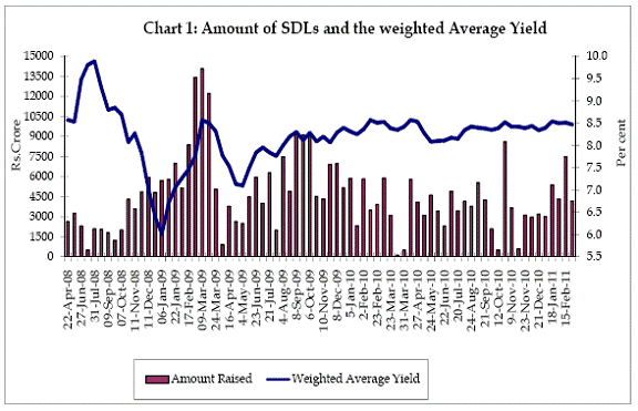
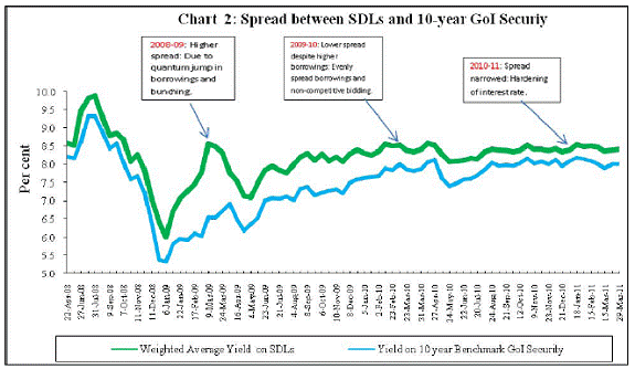
^*The year 2006-07 was marked by a switch over to the auction based issuances of the State Development Loans. Presently, India’s sub-national debt market can at best be regarded at a nascent stage of development compared to other advanced economies. With an increasing emphasis on fiscal decentralisation, it is expected that States would progressively depend more on market-based avenues of raising resources for meeting their financing requirements. Against this backdrop, it is important to examine the impact of various factors that may influence the yield spreads of State government securities, thereby affecting their overall borrowing costs. In order to examine this aspect, an attempt is made to identify the determinants of yield spreads between the State and Central government securities in a panel data framework as has been used in several cross-country studies. This study carries forward this framework to examine the potential impact of fiscal as well as market related factors on the yield spreads of 27 States/UT in India. The results indicate that the conventional deficit indicators, viz., revenue deficit, gross fiscal deficit and primary deficit, do not seem to have played a significant role in determining the yield spreads during the period 2006-07 to 2010-11. However, States with larger dependence on central transfers, mainly the special category States, appear to have benefited in terms of lower spreads. In contrast to fiscal performance variables, market related variables like tradability, size of issuances, frequency of accessing the market and interest rate environment are found to be better in explaining the yield spreads between the Central and State government securities. Therefore, investors, prima facie, do not seem to differentiate among the States based on their deficit indicators. Furthermore, States’ implicit commitment in correcting any temporary slippages in fiscal performance under the ‘Fiscal Responsibility legislations’ also adds to the confidence of market participants.

JEL classification: E43 E62 H63 H74

Keywords: Interest rates, Fiscal policy, debt management, State borrowing

Introduction

A growing trend globally is towards fiscal decentralisation which has necessitated the sub-national tiers of the government to access the market resources at competitive costs. In this context, the development of sub-national debt market assumes importance. The issuances of sub-national governments bonds dominate in the United States, Germany, Japan, Canada, China and Spain. However, the Indian sub-national debt market is still in a nascent stage of development as all State governments migrated fully from the tap-based system to auction-based issuances of market borrowings only in 2006-07.

A notable feature of the sub-national debt market in other economies is that the yield spreads relative to national debt are influenced by fiscal performance of sub-national entities as well as market conditions. Country experiences differ markedly. While the existence of deep and competitive capital markets in the US ensures that the cost of borrowing is directly related to the creditworthiness of sub-national governments, the cost structure of bond issuances in developing countries may not fully reflect the creditworthiness of sub-national governments.

Notwithstanding the fact that the State debt market is yet to be fully developed in India, there are signs of progress with increasing market participation in both primary and secondary segments. This reflects inter alia the increasing investors’ confidence backed by the implementation of rule-based fiscal consolidation at the State level from 2004-05 onwards. Therefore, one would expect market participants in State government securities to factor in the fiscal strength of the States, besides the market conditions, in their pricing and yield calculations. The empirical literature suggests that the spreads should reflect both credit risk premium (related to deficit and debt position of sub-national governments) and liquidity risk premium (linked to marketability/tradability of securities) charged by market participants for sub-national bond issuances. Schuknecht, Hagen and Wolswijk (2009), based on their analysis of data for bond yield spreads relative to an appropriate benchmark for the period 1991-2005, observe that risk premia, incurred by national governments of European Union (EU) member states, responded positively to debt and deficit levels. Lehman (1999) showed that the yield spreads on bonds issued by the sub-national governments in Australia, Canada and Germany over Central government bond yields depend positively on the ratio of state debt to GDP.

Against this background, the present study attempts to test whether fiscal and debt positions of States impact their cost of market borrowings. The objective of the study is two-fold. First, what explains the yield spreads between the securities issued by the Central and State governments? Second, does the market differentiate between the States based on their fiscal and debt positions at the time of subscribing to their securities? The study has been divided into five sections. Section I presents a review of empirical studies relating to determinants of cost of borrowings and spreads on sub-national bonds. Section II traces the market and policy related developments having bearing on the States’ debt market in India including the behaviour of yield spreads on State government securities. Section III dwells upon the methodology and data sources used in the Study. An empirical analysis undertaken to identify the factors that explain the yield spread between the Central and State government securities is covered in Section IV, while summary findings are presented along with policy implications in Section V.

I. Spread of Sub-national Bonds : Cross-country Experience

Literature available on the subject shows that spreads on the bonds of sub-national governments are influenced by a number of factors. First and the foremost factor is the fiscal performance of sub-national governments. Supporting this hypothesis, various studies [e.g., Capeci (1991, 1994); Alesina, De Broeck, Prati, and Tabellini (1992); Goldstein and Woglom (1992); Bayoumi, Goldstein and Woglom (1995) and Poterba and Rueben (1999)] showed that sub-national governments in the US paid risk premia in the bond market which was largely determined by their fiscal performance indicators. Studying the borrowing costs at a sub-national level in the US, Bayoumi, Goldstein and Woglom (1995) found yield rates to increase with the level of borrowings disincentivising the sub-national governments to go for excessive borrowings. It is observed that the yield spreads increase gradually up to a certain level of debt but show a steep and non-linear rise as the debt sustainability issue assumes significance at higher levels of debt. It implies that the States showing irresponsible fiscal behaviour would eventually witness higher borrowing costs in the market.  On the contrary, States with tighter anti-deficit rules and more restrictive provisions on the authority of State legislatures to issue debt incur lower interest burden (Poterba and Rueben, 1999). The borrowing cost is found to be higher in States with limited revenue enhancing measures while it is lower for States having expenditure limits in place. Booth, Georgopoulos, Hejazi (2007) also drew the same conclusion for Canada. De Mello Jr. (2001) pointed out that the policies aimed at disciplining sub-national finances, as part of the process of fiscal decentralisation, also tend to reduce sub-national borrowing costs. Bernoth, von Hagen and Schuknecht (2004) also argued that the State governments, with less fiscal sovereignty and lower tax collecting capacities than the national governments, are likely to pay larger default risk premia on their bonds.

The extent of explicit or implicit federal support to the sub-national governments is also identified as one of the important factors, which impacts the yield premium demanded on the sub-national borrowings. A study by Schuknecht, Hagen and Wolswijk (2009) found that during the pre-EMU period, financial markets did not pay attention to the soundness of financial health of States, as they were expected to be bailed out by the federal government in the event of a crisis. However, their findings for the post EMU period showed that the restrictions on the debt raising capacity of the federal government under the overall fiscal framework of EMU reduced the possibility of any bailout package for the State governments and fiscal health considerations have since assumed significance. Somewhat similar results were found for Canada, where equalisation transfers played a major role in finances of some of the provinces. Expecting that these provinces would, in any case, get transfers under the fiscal equalisation provision, financial markets did not charge much risk premia even if their deficit levels were higher than those of other provinces. However, the smaller provinces were found to be paying high liquidity premium on their debt. In a study on sub-national governments in Germany, Schulz and Wolff (2008) argued that despite strong revenue equalisation mechanism and several cases of bailouts by the federal government, different sub-national governments are treated differently in bond markets depending on the size of bond issuances, bond issuing strategies and liquidity of their bonds. The debt levels were, however, found to have a marginal impact on the yield spreads of sub-national bonds in Germany. Heppke-Falk and Wolff (2008) found evidence that the assured support from the national government, in one way or the other, reduces the yield spreads but does not fully explain the yield spread differentials between the sub-national governments.

As regards the determinants of yield spreads between bonds of sub-national and national governments, it is observed that apart from the factors specific to sub-national governments, other advantages enjoyed by the national governments also seem to play an important role. In most of the countries, the State governments have limited tax raising powers relative to their expenditure obligations. Therefore, they are expected to pay a risk premium in excess of the national governments. Examining the yield spreads between bonds issued by sub-national and respective national governments in Australia, Canada and Germany, Lemmen (1999) showed that the yield spreads moved positively with debt-GDP ratios of sub-national governments.

Booth, Georgopoulos and Hejazi (2007) and Schuknecht, Hagen and Wolswijk (2009) found that the relative position of outstanding debt of sub-national and national governments determined yield spreads in Canada.  In fact, the latter study provided evidence that the provinces paid a risk premium of about 0.30 basis points for every one percentage point increase in their debt ratios relative to the national government’s debt-GDP ratio. Contrary to this, a study by Galvani and Behnamian (2009) found that unlike the US bond market, the yield spreads between federal and provincial bonds of similar maturities in Canada were plain white noise and were persistently insignificant. The differential behaviour of market players in the US and Canadian debt markets is attributed to differences in perception on federal bailout of sub-national jurisdictions in both the countries. For Canada, the observed homogeneity of the federal and provincial yields could perhaps be due to market’s confidence regarding an implicit bailout for provincial debt instruments in distress.

II. Trend in Spreads on Securities of State Governments in India

In India, the dated securities of both the Centre and the State Governments are issued by the Reserve Bank. Since 2006-07, the issuance of State Governments securities has been entirely through the auction route. The Reserve Bank, in consultation with the Government of India, issues an indicative half-yearly auction calendar for Central government dated securities. The calendar provides details relating to the amount of borrowing, the tenor of security and the likely period during which auctions are to be held. However, there is no formal calendar for issuing the State government securities (State Development Loans and henceforth SDLs), though the level of (gross) market borrowings of State governments during a particular year is decided by the Central government, in consultation with the State governments. On fixation of their market borrowing limits, the State governments indicate their borrowing requirements from time to time to the Reserve Bank which arranges for auction of SDLs by bunching them together to achieve scale economies.

Till 1998, the Reserve Bank used to complete the combined open market borrowings of all the States generally in two or more tranches through issuance of SDLs with a pre-determined coupon and notified amounts for each State. In 1998-99, States were allowed to enter the market individually to raise resources using the auction method or tap method (with pre-determined coupons but without pre-determined notified amounts) with a view to providing scope of accessing funds at market rates for better managed States. The auction method could be used to the extent of 5 to 35 per cent of the allocated market borrowings (subsequently raised to 50 per cent), at the discretion of the State. To avoid the risk of under-subscription, the Umbrella Tap Tranche method was introduced during 2001-02. Under this method, after receiving the concurrence of States, the Reserve Bank used to indicate the names of States participating in the tap, the aggregate targeted amount to be raised and the coupon – the latter uniformly fixed for all the States. The targeted amounts in respect of individual States were not separately announced. Up to December 2002, the tap used to be normally kept open till the targeted amount was received for each State. In January 2003, it was decided to close the tap at the end of the second day even if the targeted amount was not mobilised (Annex I).

Until 2001, under the traditional tranche method, pre-announced coupon was normally fixed at around 25 basis points (bps) over and above the Government of India (GoI) securities of corresponding tenor. However, as interest rates fell sharply in 2000-01, and yield differences started emerging between liquid and illiquid GoI papers, it became difficult to complete the market borrowing programme (MBP) of the States at these spreads. From 2001, such spreads increased to around 50 bps. However, the system of a fixed uniform coupon did not provide any cost advantage to fiscally better managed States. Therefore, States were encouraged to move to the auction system in a gradual manner, based on the premise that competitive coupons could emerge in a market-oriented system. Notwithstanding the introduction of the auction system for SDLs in 1997, the complete switch-over to this system for raising market borrowings has taken place only from 2006-07 onwards.

With the auction-based issuances of SDLs, the yield spreads have since become variable, and exhibit differences across the States, which could be attributed to market and fiscal conditions.  During 2006-07, the spreads on SDLs (in the primary auction) ranged between 27-56 bps over and above the secondary market yield on GoI securities of corresponding tenor.

As States’ dependence on market borrowings for financing GFD increased significantly to the extent of 71.5 per cent during 2007-08, total issuances of SDLs were higher by 225.5 per cent (from Rs.20,825 crore in 2006-07 to Rs.67,779 crore in 2007-08). Reflecting the increase in average size of issuances by States, the weighted average spread for all States increased to 48 bps in 2007-08 as compared with 38 bps in 2006-07. During the last quarter of 2007-08, the spread increased further as the liquidity conditions in the system came under pressure, following aggressive borrowings by the State Governments. Therefore, States which issued SDLs during the last three auctions held during the year witnessed higher yield spreads ranging between 60-89 bps.

In 2008-09, higher borrowing levels of both Centre and the States impacted the overall yield rates in the market. The States were allowed to raise additional market borrowings to the extent of 0.5 per cent of their GSDP in 2008-09. Consequently, the gross market borrowing of the States increased by 74.3 per cent to Rs. 118,138 crore during 2008-09.  Furthermore, a noteworthy feature of the conduct of State market borrowings during the year was the scheduling of issuances primarily during the second half of the year (accounting for about 86.6 per cent of the gross annual borrowings of the States) with the bunching being particularly sharper during the fourth quarter of 2008-09 (accounting for 65 per cent of gross borrowings).  Consequently, the yield spread increased from a low of 26 basis points in the auction held on September 25, 2008 to 104 basis points on December 23, 2008. Notwithstanding some corrections in early January 2009, the spreads widened further to reach 204 basis points on March 9, 2009. For the year as a whole, the yield spreads widened to 21-236 basis points despite easing of liquidity conditions. The firming up of yields and widening of yield spreads of SDLs during 2008-09, despite easing of policy rates, reflected the pressures emanating from a quantum jump of States market borrowings and bunching of bond issuances during the latter half of the year (Chart 1).

During 2009-10, the SDLs issuances were more evenly spread throughout the year. Although the weighted average yield on SDLs was higher at 8.11 per cent in 2009-10 (7.87 per cent in 2008-09), there was a sharp decline in spreads as compared with that in 2008-09  and remained in the range of 45 -129 basis points. On the whole, the weighted average spread stood lower at 86 bps during 2009-10 as compared with a higher spread of 122 bps during 2008-09. The lower spread during 2009-10 reflected introduction of non-competitive biddings and also to some extent due to the introduction of embedded derivatives in the issuance of SDLs.¹

During 2010-11 , States have raised lower level of SDLs at Rs.1,04,039 crore as compared with Rs.1,31,122 crore raised during the previous year. Reflecting the hardening of interest rate environment, the weighted average yield increased to 8.39 per cent as compared with 8.11 per cent for the previous year. However, an interesting feature is that the weighted average spread declined to 45 bps during the year as compared with 86 bps during the previous year. Lower spread during 2010-11 may be due to varied factors including lower market borrowings on account of comfortable cash position of the States, lower average isssunace size at Rs.708 core as comopared with Rs.825 crore during the previous year, lower volatility in the yield movement of 10-year benchmark GoI securities in the secondary market (measured in terms of standard deviation), perceived bidding by the investors with a view to keep it in the HTM category, using the State government securities as collateral for availing credit under LAF, etc. However, the tight liquidity conditions prevailing in the financial market  during the year has not detered the buoyancy in the primay auctions of SDLs, which reflected in the form of lower spread coupled with higher bid-cover ratio.

Overall, the yields on SDLs reflect the general interest rate regime and the spread varies depending on a host of factors including the monetary policy initiatives from time to time. During the initial phase, which was characerised by higher interest rates, the spread was moderate (Chart 2). However, despite the general interest rate regime easing thereafter, the spread settled at a higher level. During the recent period, the call rates have firmed up significantly but the bond yields have not firmed up noticeably except on a few occasions. The pattern of past auctions shows that accessing the market at a right time with right size of issuance yields a right price to the SDLs, with a narrowing down of the spread.

III. Data Sources and Empirical Approach

In order to examine the relative importance of fiscal indicators and market related variables in determining the yield spreads between the Central government securities and the SDLs across States, an empirical exercise is undertaken in the panel data framework. It captures cross-sectional as well as time dimension of the State level data. Under the panel data analysis, 27 States including the Union Territory of Puducherry are covered; Orissa and Chhattisgarh have been dropped, as they have not raised borrowings in most of the years during the period of analysis.  The time period covered is from 2006-07, the year when the State governments began to raise SDLs entirely through the auction route, to 2010-11. Since the same number of time-series observations is available for each State (or equivalently but viewed the other way around, the same number of States at each point in time), a balanced panel of 135 observations (27 States x 5 years) is constructed.

Data on fiscal indicators of States have been taken from the ‘Handbook of Statistics on State Government Finances (2010)’ and also from the budget documents of the State governments for 2010-11. Data on market-related variables have been sourced from the Internal Debt Management Department (IDMD) which provided data on variables², viz., (i) relative size of market borrowings of States, (ii) State-wise yield, (iii) spread over Central Government yield and average yield of all States, (iv) size of auction and (v) number of tranches. Data on average call money rate, which is used as a proxy for market conditions and overall interest rate environment, have been compiled from the ‘Handbook of Statistics on the Indian Economy’. In addition, data on State-wise turnover of government securities in secondary market have been sourced from the Clearing Corporation of India Ltd.

For the empirical analysis, State-wise yield spread on SDLs has been calculated as a difference between the yield on State government security (Y_it) and yield on GoI dated securities (Y_ct) of 10 years maturity.

Instead of using auction-wise data on yields, the study has been based on State-wise annual weighted average yields and spreads thereof. Since the data on State fiscal indicators are available only on an annual basis, it seems appropriate to use annual data, instead of auction-wise data.

Before examining the relative importance of fiscal performance and market related factors in influencing the yield spreads of State government securities over that of the Central government, it is important to list out the factors that can have a bearing on the yields of State government securities. Among the state-specific factors, four key indicators, viz., revenue deficit, primary deficit, fiscal deficit and debt-GSDP ratio (DGSDP), are used in alternate equations. Since these four variables are expected to be highly correlated with each other, their simultaneous inclusion in a single equation can lead to the problem of multicollinearity. Theoretically, it is expected a priori that the States with high deficits/DGSDP ratios may have to raise borrowing at higher yields and vice versa. In addition to the key fiscal deficit indicators, States’ dependence on Central transfers is taken as another important determinant of yield spreads, as has been found in similar studies on Canada and Germany. To capture this determinant, the ratio of Centre’s current transfers to each State (including tax devolution and grants) to their respective revenue receipts is included as a variable.

In addition to the State-specific fiscal variables, market conditions also impact the yield spread on State Government Securities. Five market related variables, viz., average size of issuance, number of tranches, call money rate, number of trades in secondary market and share of a State in total issuances of securities of States have been chosen. In addition, a dummy variable for special category States has been included (Table 1).

On a priori basis, it is expected that more frequently a State (or States as a group) comes into the market for raising borrowings in a year, higher should be the yield spread. This aspect has been captured by using the number of tranches (NT) as a variable. Average call money rate is used to capture the interest rate environment and market conditions when the States approach the market for borrowings. Average call money rate (ACMR) is calculated as an average of call rate prevailing during the five days (day of tranche, two days before and after the tranche). Average size of SDL issuances is also expected to positively influence the yield spread. Most of the States with small size issuances are special category States. Given the fact that these States largely depend on the Centre for their revenue receipts (70 per cent of revenue receipts), it is quite possible that the market participants may not demand high risk premium on their securities.  The log of average size of issuance (LAVSZI) is used, as this variable is found to be positively skewed. Another variable that is expected to influence the yield spread is tradability of State government securities. The number of trades (NOT), i.e., number of times the securities of each State was traded in the secondary market is included in the model. It is expected that higher the tradability of a security, lower will be the illiquidity premium and therefore lower spread. The relative share of each State in total annual issuances (RS) by the State governments is another state-specific variable in the model. One would expect that higher the share of a State, higher would be the yield spread on its securities. Dummy variable is used to test whether the yield spreads on securities of special category States vary vis-à-vis non-special category States. Therefore, dummy variable 1 is used for special category States and 0 for non-special category States.

In a panel data analysis, three approaches can be followed. These are pooled least square (without assumption of fixed effect or random effect), fixed effect model and random effect model. The simplest way to deal with the panel data is to estimate a pooled regression using OLS, which involves estimating a single equation on all the data together, so that the dataset for variables (both dependent and explanatory variables) is stacked containing all the cross-sectional and time-series observations. Even though this approach is simple and does economise in terms of degrees of freedom, its major limitation is the implicit assumption that the average values of the variables and the relationships between them are constant over time and across all the cross-sectional units. Therefore, this approach does not make full use of this rich structure of panel data (Equation 1). In addition to pooled regression analysis, there are broadly two classes of panel estimator approaches that are commonly used. These are fixed effects models and random effects models.

To test for the presence of statistically significant group and/or time effects, fixed effects model is found to be more suitable. The simplest type of fixed effects model allows the intercept in the regression model to differ cross-sectionally, while all the slope estimates are fixed both cross-sectionally and over time. Under fixed effects model, the error term uit, can be decomposed into an individual specific effect, μ_i, and the ‘remainder disturbance’, v_it, that varies over time and across sections (capturing everything that is left unexplained about y_it). Here μ_i encapsulates all of the variables that affect y_it cross-sectionally but do not vary over time (Equation 2). An alternative to the fixed effects model is the random effects model which provides for different intercept terms for each unit of cross-section but these intercepts remain constant over time, with the relationships between the explanatory and dependent variables assumed to be the same both cross-sectionally and temporally. Under the random effects model, the intercepts for each cross-sectional unit are assumed to arise from a common intercept α (which is the same for all cross-sectional units and over time), plus a random variable ei that varies cross-sectionally but is constant over time. ei measures the random deviation of each entity’s intercept term from the ‘global’ intercept term α (Equation 3) [Brooks, 2008].

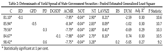
In the above equations, i represents i^th crosssection and t represents time. In the present study, pooled least square and fixed effects models are used. Since the cross section units (i.e., States) in the sample effectively constitute the entire population and are not randomly selected from the population, a fixed effect model appears to be appropriate in the context of our analysis.

IV. Determinants of Yield Spreads: Empirical Evidence

As stated in the foregoing section, pooled least squares method and fixed effects model are attempted in this section to identify the determinants of spread between the yields on securities of the Central and State governments. Empirical findings based on a pooled generalised least squares regression method are presented in Table 2.

Under the pooled estimated generalised least square regression (EGLS), it is found that the key variables representing the fiscal performance of States do not seem to explain the yield spread on State government securities. In none of the four equations including the four fiscal variables (viz., RD, GFD, PD and DGSDP), regression coefficient of fiscal variables is statistically significant. It shows that States’ fiscal performance perhaps is not influencing yield spreads on State government securities. In contrast, most of the market related variables turn out to be statistically significant at 1 per cent and have the expected sign in most of the equations. In all the four specifications, the average size of bond issuance of States has shown a statistically significant influence over yield spreads. As was hypothesized, the relationship between spread and the average size of issuance appears positive. It shows that the yield spreads tend to increase with increases in the average size of bond issuance. However, due to the log transformation, the LAVSZI variable has to be interpreted carefully. It is found that with a 10 per cent increase in AVSZI, the yield spread increases by 78 basis points.³ The coefficient of another market related variable, i.e., NOT, representing the extent of tradability of State government securities, also turns out to be negative and statistically significant. It indicates that States whose securities are traded more frequently in the secondary market are able to raise resources at a relatively lower cost, reflected in lower spread level.  As was expected, the special category States seem to be borrowing at a lower cost as yield spreads are found to be lower than those of non-special category States. However, the yield spread differential observed between special and non-special category States is not statistically significant. The impact of interest rate environment on yield spread appears to be statistically significant. It has been found that the yield spread between central and State government securities declines when the average call money rate (ACMR) reflecting the tightening of liquidity conditions narrows yield spreads.

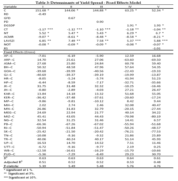
The fixed effect model broadly confirms the relative importance of variables as estimated under simple pooled EGLS method. Since the fixed model includes individual intercept terms, dummy variable used under pooled EGLS were dropped from the specification of equation. Instead, CT is included to examine whether States with heavy dependence on the Centre through transfers are able to attract better pricing leading to lower yield spreads on their SDLs. It is found that the coefficient of RD is not only inconsistent with a priori expectation but also statistically insignificant. On the other hand, the respective coefficients of GFD and PD, albeit showing consistent signs, are found to be statistically insignificant. However, under fixed effect model, the coefficient of DGSDP shows statistical significance at 1 per cent reflecting the importance of debt sustainability. It is also found that the States which largely depend on Central transfers perhaps pay lower spread. CT variable is found to be negative and statistically significant at 5 per cent or 10 per cent level. To some extent, it supports the earlier finding (under EGLS) that spreads are lower on securities of special category States which largely depend on the resource transfers from the Centre and, therefore, market participants seem to perceive their fiscal performance relatively stable as compared with other States.

All market related variables, viz., NT, ACMRI, LAVSZI and NOT show signs which are consistent with those found under simple pooled EGLS and are mostly statistically significant at accepted levels. The coefficient of relative share of a State in total issuances (RS) by the State governments does not show any statistical significance. Furthermore, the explanatory power of the model improves significantly under the fixed effects model. F statistic also confirms joint statistical significance of coefficients of variables included in the different specifications. State specific fixed effects show that the intercept term varies across States (Table 3). Significant differences are observed in State specific intercepts, which shows that there are certain State-specific factors, other than those included in the model, which are playing a role in explaining the yield spreads across the States. In order to test the joint significance of the fixed effects estimates, redundant fixed effect test is used. The test shows that the State-specific fixed effects are statistically significant and not redundant (Table 4). 

In short, the key deficit indicators which are generally monitored to gauge the fiscal performance do not seem to explain the yield spreads across States. The analysis lends some support to the argument that the States with higher debts pay higher yields as compared with other States. Similarly, there is also evidence that Central transfers to the States help them to raise borrowings at lower spreads. Notwithstanding the low explanatory power of fiscal variables in variation in yield spreads, the importance of rule-based fiscal policy during the period of our analysis cannot be undermined. In fact, the fiscal consolidation being pursued by the States might have provided confidence to the market whereby temporary deviations in deficit levels observed during crisis years were expected to be corrected over the medium-term. Furthermore, it needs to be noted that fiscal discipline at the State level is progressively becoming incentivised by the Finance Commissions, which may have acted a source of comfort for the market. It is corroborated by the fact that after witnessing fiscal stress during the period of global financial crisis, most States seem to have reverted to path of fiscal consolidation as evident from lower deficit ratios during 2010-11 and 2011-12.

V.  Conclusion and Policy implications

The empirical analysis in this study has found that the market participants in State government securities market have, by and large, not factored in the conventional fiscal performance of the States in determining the yield spread during the period 2006-07 to 2010-11. As this coincides with a rule-based fiscal consolidation, this feature could perhaps indicate investors’ confidence that the States are committed to bringing about fiscal consolidation and would reduce their deficit levels and bring them in line with the medium term targets. Therefore, coefficients of most of the fiscal performance variables are found to be statistically insignificant in determining the yield spreads. On the other hand, another fiscal performance variable, viz., debt-GSDP ratio is found to be statistically significant in one out of 10 equations. In overall terms, therefore, investors, prima facie do not seem to attach any credit risk premium to State debt issuances based on deficit indicators. However, the special category States seem to benefit vis-à-vis non-special category States perhaps because of their heavy dependence on the Centre in terms of transfers (mainly grants) which lends stability to their fiscal performance. This, to some extent, is supported by the findings under the FE model that the States with greater share of Central transfers in revenue receipts (mainly the special category States) benefit in terms of lower spreads. In contrast, market related variables have a significant influence on the yield spreads on State government securities. States with higher average size of issuance have to pay higher yields; States which approach market more frequently also pay higher yields on their borrowings as variable NT capturing the number of tranches for each State is positive and statistically significant. States whose securities are traded more frequently pay lower spreads as compared with other States. It is also found that in the phase of high interest rate environment, the yield spread between the Centre and State government securities narrows down.

In the light of empirical findings in this study, a few policy implications that emerge are as follows.  As the yield spread varies positively with the size of the issues, there is a scope for the States to work out the optimum size of the issuance, keeping in view their financing requirements. Similarly, the finding that States approaching the markets more frequently have to pay higher yields as compared to other States points towards devising a better forecasting mechanism of revenue and expenditure flows so that borrowings are only need-based. These may help the States in economising their borrowing cost. Introducing a calendar for States borrowing programmes on the lines of Central borrowing programme may also facilitate States accessing market at lower cost.

To sum up, the study demonstrates that markets do not differentiate between the borrowings of various States, notwithstanding their very different financial conditions. Nonetheless, the criticality of rule-based fiscal consolidation of the States cannot be undermined. The prevalence of a rule-based fiscal policy across States during the period of analysis of this study appears to have provided confidence to investors regarding their commitment to fiscal discipline.  Nevertheless, fiscally better managed States may explore feasibility of disseminating their best fiscal practices through various channels to attract lower yield. Furthermore, States need to carry forward their approach towards fiscal consolidation by amending FRBM Acts so that market investors remain assured of sound State finances.

^@ Dhritidyuti Bose (dbose@rbi.org.in), Rajeev Jain (rajeevjain@rbi.org.in) and L. Lakshmanan (llakshmanan@rbi.org.in) are Director, Assistant Adviser (Department of Economic and Policy Research), and Assistant Adviser (Internal Debt Management Department), respectively, in the Reserve Bank of India.

^*They are grateful for the encouragement and comments received from Smt. Balbir Kaur, Adviser, DEPR. The paper was presented in the 24th Conference of State Finance Secretaries at the Reserve Bank of India on May 24, 2011. Views expressed in the paper are entirely personal of the authors and not of the institution they belong to. Errors and omissions, if any, are the sole responsibility of the authors.

¹With an intention to raise resources at a lower rate of interest, one State Government raised SDLs with put option during 2009-10, which could be exercisable by the investors after the completion of 4-5 years from the date of issue. Accordingly, the spread for that State was just 63-65 bps in that auction as against the spread of 97-111 bps settled for other States. Though, the put option is a way of price discovery and aimed at reducing the interest burden of the Government, there would be rollover risk and bunching of repayment obligations in the short term if investors choose to exercise the put option.

² Auction-wise details are available in the public domain through press releases. Further, aggregate details are also available in the Bank’s publications such as Annual Report, State Finances: A Study of Budgets and Handbook of Statistics on the Indian Economy.

³ Coefficient for LAVSZI is in range of 8.0 to 8.5. Even though by log transformation LAVSZI shows linear impact on spreads but the estimated effects of average size of issuance is not linear. If impact of 10 per cent rise in average size of issuance is to be calculated, the relevant coefficient should be interpreted as 8.21 (Log 1.10) =0.78.

References

Alesina, A., M. De Broeck, A. Prati, and G. Tabellini (1992): “Default Risk on Government Debt in OECD Countries,” Economic Policy, Vol. 7, No. 15, 427–451.

Bayoumi, T, M. Goldstein, and G. Woglom (1995), “Do Credit Markets Discipline Sovereign Borrowers? Evidence from U.S. States,’ Journal of Money, Credit and Banking, Vol. 27, pp.1046–59.

Bernoth, Kerstin; Jürgen von Hagen; Ludger Schuknecht (2004) “Sovereign Risk Premiums in the European Government Bond Market”, ECB Working Paper No. 369.

Booth, Laurence; George Georgopoulos and Walid Hejazi (2007), “What drives provincial-Canada yield spreads?, Canadian Journal of Economics, Vol. 40, No. 3.

Brooks, Chris (2008), Introductory Econometrics for Finance, Cambridge University Press.

Capeci, J. (1991): “Credit Risk, Credit Ratings, and Municipal Bond Yields: A Panel Study,” National Tax Journal, Vol. 44, No. 1, pp. 41–56.

Capeci, J. (1994): “Local Fiscal Policies, Default Risk, and Municipal Borrowing Costs,” Journal of Public Economics, Vol. 53, No.1, pp. 73–89.

De Mello Jr , Luiz R. (2001), “Fiscal Decentralization and Borrowing Costs: The Case of Local Governments”, Public Finance Review, Vol. 29, No. 2, pp.108-138.

Fasten, Erik R. (2008), “On the Sustainability of Sub-national Government Finance - A Panel Data Approach”, Department of Economics and Management, Humboldt University, Berlin.

Galvani, Valentina and Aslan Behnamian (2009), “A Comparative Analysis of the Returns on Provincial and Federal Canadian Bonds” University of Alberta, Department of Economics Working Papers No. 2009-7.

Heppke-Falk, K. and Guntram B. Wolff (2007), “Moral Hazard and Bail-Out in Fiscal Federations: Evidence for the German Länder”, Deutsche Bundesbank Discussion Paper No. 7.

Lemmen, J. (1999), “Managing Government Default Risk in Federal States”, Financial Markets Group, Nijmegen, Netherlands. Special Paper 11.

Poterba, J. and K. Rueben. (1999), “State fiscal institutions and the U.S. Municipal Bond Market,” NBER Working Paper No. 6237.

Schuknecht, Ludger; Jürgen von Hagen and Guido Wolswijk (2009), “Government Risk Premiums in the Bond Market EMU and Canada”, European Journal of Political Economy, Vol. 25, pp.371-384.

Schulz, Alexander and Guntram B. Wolff (2008), “The German sub-national Government Bond Market: Structure, Determinants of Yield Spreads and Berlin’s Forgone Bail-out”, Jahrbücher für Nationalökonomie und Statistik, Vol. 229, No.1.

Annex I : Chronology of Developments in the Issuance of SDLs