 IST,
IST,


Report Of The Technical Advisory Group On Development Of Leading Economic Indicators For Indian Economy
|
REPORT OF
THE
RESERVE BANK
OF INDIA Contents
Report of
the Technical Advisory Group on Section – I I.1 Genesis of the Group 1.1 In view of the need for monitoring the movements of the Indian economy on a regular basis it has been felt necessary to develop coincident, leading and lagging economic indicators based on appropriate methodology and the international best practices. Accordingly, the Reserve Bank of India has set up a Technical Advisory Group on 'Development of Leading Economic Indicators for Indian Economy', vide, Memorandum issued by Deputy Governor, Dr. Rakesh Mohan on March 1, 2006 (Annex I).
1.2 The constitution of the Technical Advisory Group is as follows:
1.3 The Terms of Reference of the Technical Advisory Group are as given below: (i) To suggest a feasible methodological framework for construction of co-incident, leading and lagging indicators and composite index for the Indian economy, with a view to assist monetary policy formulation, and to guide and oversee its implementation. (ii) To recommend modalities of outsourcing the work for construction of indicators by appropriate external agency or institution, including scope of work and deliverables. (iii) To evaluate the work of the external agency and recommend its acceptance by the Bank. (iv) Any other issue as deemed necessary for development of indicators on business cycle. 1.4 The memorandum authorized the Technical Advisory Group to co-opt any other person/s for specific deliberations. I.2 Scheme of the Report 1.5 The Group deliberated on several issues regarding the development of the leading economic indicators during the two meetings held in Mumbai. In the First Meeting, graced by Deputy Governor Dr. Rakesh Mohan, the issues regarding the selection of reference series and methodology for construction of the composite leading economic indicators were discussed. In the Second Meeting chaired by Executive Director Dr. R. B. Barman, the empirical results, based on the suggestions received in the First Meeting were discussed. Based on these deliberations and the background empirical work undertaken, the Group finalised the Report. The Report is organized as follows. The Report is divided into six sections. Section II provides a brief description of Business Cycles. Section III covers a brief discussion about the methodologies. Section IV discusses the application of leading economic indicators, both, international and Indian and experiences gained. The details of empirical work done for estimation of cyclical components and construction of the Composite Index of Leading Indicators using growth cycle and growth rate cycle methodologies are discussed in Section V. In Section VI, Composite Index of Coincident Indicators is prescribed. Section VII concludes with Recommendations of the Group. I.3 Acknowledgements 1.6 The Group would like to thank Dr. Rakesh Mohan, Deputy Governor, Reserve Bank of India for his invaluable insights made during the First Meeting. The Group is thankful to Dr. A.K. Tripathi, Assistant Adviser and Shri S. Bordoloi, Research Officer of the Forecasting Division for their untiring contribution towards completion of this Report. Perhaps, without their support, the Report would not have been completed within stipulated time. The Group is thankful to the Principal Adviser, Department of Statistical Analysis and Computer Services for providing all the facilities for perusing the work and the arrangements for the Meetings. Section –
II II.1. Definition 2.1 The economic activity generally oscillates between the phases of expansion and contractions. Understanding the periodicity of expansionary and contractionary phases of economic activity has become the focus of macro-economic research, under the purview of business cycle. The study of business cycle enables the policy makers to trigger timely appropriate policy action in order to bring back the economic system to the desired path. 2.2 The classical definition of business cycles, as proposed by Burns and Mitchell (1946), is 'Business cycles are a type of fluctuations found in the aggregate economic activity of nations that organize their work mainly in business enterprises: a cycle consist of expansions occurring at about the same time in many economic activities, followed by similarly general recessions, contractions and revivals which merge into the expansion phase of the next cycle; this sequence of changes is recurrent but not periodic. In duration, business cycles vary from more than one year to ten or twelve years; they are not divisible into shorter cycles of similar character with amplitudes approximating their own'. 2.3 These observations form the basis of the classic definition of business cycles in market economies established by Mitchell in 1927. The key features are:
2.4 There are three main approaches to business cycle analysis, viz., Classical Cycles, Growth Cycles and Growth Rate Cycles.
2.5. Practically, extraction of 'growth cycles' is a difficult task due to certain problems in estimating trend. Though there are several techniques, such as, Hodrick-Prescott (HP) 3 filter, Band- Pass (BP)4 filter, Phase Average Trend (PAT) etc., which are widely used for the purpose, the general consensus is that measuring 'growth cycles' accurately on real-time basis is practically difficult. 2.6. For a measurement of the business cycle, one has to observe a benchmark series, known as the reference series. The reference series encompasses the overall economic activity and could be adopted for policy purposes. Such a series may be a single series (indicator) or it may be a combination of certain economic series. A single indicator may at times produces false signals, and hence the latter may be preferred. To provide a more comprehensive measure of economic activity, the Composite Index of Coincidental Indicators (CICI) has been developed in many countries. The CICI are based on a basket of economic indicators, which represents the current economic activity. 2.7. Broadly, there are three types of indicators, viz., leading, coincidental and lagging indicators. The leading index, which combines the series that tend to lead at business cycle turns, provides a measure of expectation in the near future. The coincident index, comprising of indicators that measure the current economic performance is used to represent the level of current economic activity. On the other hand, the lagging index is a combination of indicators that reach their turning points after the peaks and troughs of the coincident indicators, helps to clarify and confirm the underlying pattern of the economic activity. declined in the fourth quarter. This violates the 'two-down-quarter rule'. (Extracted from Dua and Banerji (2001)).2Klein, P.A. (1998) 3See Annex-II.A. 4See Annex-II.B. II.2.
Identifying Potential Economic Indicators 2.9.Generally indicators are identified based on some economic rationales. As suggested by De Leeuw (1991), selection of a leading indicator may be justified by one or more of the following five rationales.
2.10. Silver (1991) suggested the following six criteria to judge the quality of an indicator. The quality of an indicator is judged through some pre-defined criteria, set as per need and purpose of the analysis. In determining the usefulness of an indicator, the traditional National Bureau of Economic Research (NBER) approach applied the following six criteria to a series:
Under this strategy, a score is awarded for each criterion and an overall score for each indicator under consideration is worked out. The indicators to be used for forecasting the overall economic activity are then chosen from these indicators on the basis of their overall scores. 2.11. The selection of individual indicator to construct composite indicators follows certain steps5
2.12. The appropriateness of an indicator may also be assessed, through its turning points, vis-à-vis., the reference series. For assessing the appropriateness of a Leading Indicator (LI), the point-to-point lead periods may be estimated. The standard deviation of these point-to-point leads will give the extent to which the estimated lead period of the LI is reliable. The lead period of a LI may be estimated by measuring median or mean lead. For evaluation of the length of the lead, the median lead is preferred to the mean, as the mean lead is strongly affected by extreme values. 5Simone (2001). II.5. Constructing Composite Indicator Index 2.13. The construction of leading, coincident and lagging indicators is important from the viewpoint of forecasting business cycles, particularly its turning points. Knowledge about the turning points is particularly important as most of forecasts go wrong at these points because the projections are generally based on linear models and the linear relationship characterized by a particular linear model breaks down around the turning points. From the viewpoint of the monetary policy, which involves transmission lags, correct forecasting of turning points is immensely important so as to facilitate appropriate policy actions to counter overheating or excessive downturns in the aggregate economic activity.Section III 3.1. The first step involved in the estimation of the growth cycle is the adjustment for seasonality, as the seasonal movement may obscure the cyclical movements and hence needs to be eliminated first. There exist various methods for seasonal adjustments in the literature, viz., Moving Average method, X-12-ARIMA, Tramo- Seats, etc. 3.2. In the second step, one requires to estimate the trend component and eliminate it from the seasonally adjusted data. Among the various methods for estimation of the trend, the most popular method includes the Hodrick- Prescott (HP) filter, the Band- Pass (BP) filter, the Exponential Smoothing method and the Phase Average Trend (PAT). 3.3. The total area below the spectral density corresponds to the variance of the series, and the height at any given frequency provides a measure of the variance for that particular frequency. The method that explains the larger proportion of spectral mass in the range of business cycle frequencies may be selected for estimation of the growth cycles. 3.4. As the estimated cycles may have presence of volatility, some smoothing is required to sort out the short-term irregular component. Generally moving average method is applied to reduce the short-lived volatility. The moving average may be a simple equal weighted centered moving average or weighted moving average. The length of the moving average is generally determined from the standardized spectral density, at frequencies corresponding to periods of less than a year. 3.5. The smoothend series, resulting from the above three steps, are used for obtaining the growth cycles. III.2. Estimation of the Growth Rate Cycles 3.6. Growth rate cycles are the simple cyclical upswings and downswings in the growth rate of the economic activity. The growth rates are estimated as the simple annual point-to-point growth rates. 3.7. As the growth rate cycles estimated as above is expected to be quite volatile, smoothing may be required to eliminate these short-term volatile component, if required. Smoothing can be done through the application of moving average method described above. III.3. Identifying the Turning Points 3.8. Turning points for the reference series and the indicator series are determined based on the smoothed series described above. For identification of the turning points, one may adopt the Bry and Boschan rule (1971) or the Artis et al. rule (1995). 3.9. The Bry- Boschan procedure suggests the following rules for identification of the turning points:
3.10. Artis op cit. procedure is based on the following four rules, to identify the turning points:
III.4. Assessing the quality of Indicators 3.11. The mean and standard deviation of leads give partial information about the leading quality of a LI. The efficiency of a LI also depends upon its success in indicating the turning points of the target series in advance. A good indicator should predict each of the turning points in advance devoid of any false signals. A measure of the efficiency is defined as6
where η = the measure of efficiency, σ = the standard deviation of all leads of the LI with respect to the reference series, T = number of points in which the indicator leads the nearest turning point in the reference series, N = number of turning points identified in the reference series, H = number of turning points identified in the indicator. 3.12. For evaluation of the candidate Indicators for their cyclical performance, Organisation for Economic Co-operation and Development (OECD, 2006a) has set a number of statistical methods; both classical descriptive and univariate methods based on the National Bureau of Economic Research (NBER) approach and multivariate methods such as dynamic factor models. 6Cabrero and Delriue (1996).
3.13. To reduce the number of indicators a selection is performed on the results by a screening procedure based on certain criteria related to the cyclical performance of the indicators. Indicators may be included in the final set of indicators if they are accepted on more than four/ five of the following eight criteria:
3.14. The Quadratic Probability Score7 (QPS) of each indicator may also be used to evaluate the quality of the indicator. The QPS is defined as
where P denotes the predicted outcomes from a indicator and R is the observed realization in the reference series, both equal to one for a turning point and zero otherwise. N is the total number of sample observations. By construction, the value of QPS ranges between zero and two, with zero indicating perfect prediction and two indicating no single correct signal from an indicator. [H1, H2] is the prediction window, which is used to determine whether a predicted outcome represents a correct signal or a false one when it takes the value of one, and whether or not it has missed a turning point when taking the value of zero. III.5. Selection of the Leading Indicators 3.15. After identification of the turning points, the next step is the selection of the appropriate leading indicators from the set of all indicators. Selections of the indicators can be done through cross correlation analysis, spectral analysis8 or Self-Organising Maps. 3.16. The simple product correlation co-efficient between the reference series and the leading indicators gives an idea about the information contained in the indicator about the reference series. A higher magnitude of the correlation co-efficient indicates the existence of better information contained in the indicator. 7 Diebold and Rudebusch (1999).8 Bikker and Kennedy (1999). 3.17. Self-Organising Map (SOM) is generally applied for the purpose of clustering. Through the application of a SOM the indicators can be classified into different clusters, based on certain features contained in the indicators. Selection may be restricted among those indicators, which fall in the same cluster along with the reference series. III.6. Construction of the Composite Index of Leading Indicators 3.18. Composite Index of Leading Indicators (CILI) may be constructed following several competing methodologies – some in linear framework and others in non-linear framework. A few of these methodologies are discussed below: 3.19. Linear Framework:
3.19.1. An indicator that is individually co-integrated with real GDP is used as a starting point. Other indicators are added to the regression one at a time. Once an indicator is added, the expanded vector is also tested for co-integration. 3.19.2. The unrestricted models are tested to see if the contemporaneous indicators could be eliminated. If they could be, then it means that only past information for a indicator can be used to forecast real GDP. The unrestricted model that has this property is considered to be a candidate to construct a leading indicator. 3.19.3. The several models selected using this process are ranked according to the fit as well as out-of-sample forecast performance. 3.20. Non-Linear Framework
9 Stock and Watson (1991). Section
IV IV.1. International Experience 4.1. The Leading Indicator approach originates from the works of Burns and Mitchell at the NBER in the US in the mid-1930's. This was used to study macroeconomic data and forecast the waves of economic expansion and contraction. Over the years the approach was developed at the NBER under the leadership of G.H. Moore. He later founded the Economic Cycle Research Institute (ECRI). 4.2. ECRI's founder, Dr. Geoffrey Moore, established the first list of leading economic indicators of recession and recovery in 1950. The first leading indicators were: Sensitive
commodity prices The ECRI compiles leading, coincidental and lagging indicators for twenty countries all over the world, viz., the United States, Canada, France, Germany, Mexico, United Kingdom, Italy, Spain, Switzerland, Sweden, Austria, Japan, China, India, Korea, Australia, Taiwan, New Zealand, South Africa and Jordan. The growth rate cycles and business cycle, both methodologies are followed by the ECRI. The reference series is the real GDP. 4.3. The U.S. Conference Board publishes leading, coincident and lagging indices to signal peaks and troughs in the business cycle for nine countries, viz., the United States, Australia, France, Germany, Japan, Korea, Mexico, Spain and the United Kingdom, around the world. The CLI for the countries are based on the 'growth rate cycles'. 4.4. During the early 1980s, the Organization of Economic Cooperation and Development (OECD) developed its system of composite leading indicators and business cycle analysis to provide early signals of turning points in economic activity. Currently the OECD compiles CLI for 29 of its 30 member countries and for six non-members countries. The six non-members countries include India also. The OECD CLI is based on the 'growth cycle' approach. Their indicator system uses univariate analysis to estimate trend and cycles individually for each component series and then a CLI is obtained by aggregation of the resulting de-trended component. 4.5. The National Statistical Coordination Board (NSCB), Philippines, compiles the CLI for the Philippine economy. The non-agriculture component of GDP is taken as the reference series. The CLI is based on the 'growth cycle' approach. IV.2. Present status of work in the Indian context 4.6. There have been a large number of studies on indicators for the Indian economy, generally on individual basis. Select studies in the context of the Indian economy are briefly discussed here. The list of indicators for some selected studies are provided in Annexure- VI. 4.7. Chitre (1991) presented evidence of synchronous movements in respect of a large number of key economic processes including non-agricultural Net National Product, industrial production, capital formation, money stock, bank credit, etc. The study analysed 94 monthly time series for the period 1951 to 1982 in order to prepare a list of indicators for business recessions and revivals in Indian economy and studied the leads and lags of the turning points of the growth cycle in individual series in relation to the turning points of the cycle in the overall economy. The cyclical component was estimated as the ratio of the de-seasonalised and the de-trended series. Finally, eleven indicators viz., IIP-General index, IIP-Capital goods, IIP-Intermediate goods, IIP-Consumer non-durables, Production of cement, Production of electricity, Exports, Imports, Railway wagons loaded, Change in bank credit and Cheque clearance (amount) were selected after considerable experimentation to determine the reference dates giving the cyclical turning points in India's overall economic activity. The overall reference cycle was estimated based on these indicators using three different methods, viz., the diffusion index, the composite index and the first principal component index. The three indices yielded more or less similar reference dates (peaks and troughs). In the study, lead, lag and coincident indicators at peak and at trough were also identified based on the relationship between the movements of individual cycles and the reference cycle. 4.8. Dua and Banerji15 followed the classical NBER approach to estimate the reference chronologies of Indian business cycles and the growth rate cycles. The study focused on the approach for construction of composite co-incident index. The study identified leading and coincident indicators, constructed composite index for both and examined their performance for dating the recessions and to anticipate business cycle and growth rate cycle upturns and downturns. Six business cycle recessions in the Indian economy were reported. It was also observed that Indian business cycles have averaged over six years in length, with recessions averaging just less than a year and expansions just over five years. The Indian growth rate cycles were also reported. However, the details of the component series used for construction of the indicators were not published in the above study. 4.9. Hatekar16 used annual data for the period 1950-85 and described individual historical path of major macroeconomic variables and their comovements with other variables. The study tested the real business cycle proposition that nominal magnitudes and real money balances cannot be exogeneous during mechanisms of the business cycle. 15 Dua and Banerji (2001). 4.10. Gangopadhyay and Wadhwa (1997) used monthly data on IIP for the period 1975:Q2 to 1995:Q1 for obtaining the chronology of Indian business cycles using deterministic trend (annual growth rate of six per cent). They also attempted to forecast the level of annual GDP using monthly data on IIP which they argued could also be used to update the forecast of GDP especially once the data for the first half of the fiscal year is available. 4.11. Mall (1999) characterized Indian business cycles based on the non-agricultural GDP as the reference series as its cyclical components were found to have strong relation with the cyclical components of overall GDP, private consumption, investment, manufacturing output, domestic trade, IIP, private corporate sales and vale added. The turning points of IIP- Manufacturing were found to be roughly coincident with major output variables in the non-agricultural sector of the economy. A composite index of leading indicators with 14 components for IIP-manufacturing was developed with a forecast horizon of two quarters. 4.12. OECD (2006b) has recently developed a CLI for India. The CLI is developed based on the growth cycle methodology, with the monthly series of index of industrial production (IIP), excluding construction, has been taken as the reference series. Eight leading indicators, viz., Business Confidence index (NCAER), Imports, Money Supply (M1), Exchange rate INR/USD, Deposit interest rate, Share stock prices (BSE), IIP- Basic Goods and IIP- Intermediate Goods were identified as the potential indicators for computing the CLI. The CLI for India showed a median lead of only one month at all turning points over the two cycles in IIP registered since 1995.
Section V V.1. Data Aspects 5.1. The existing information base for leading indicators for the Indian economy includes national income aggregates, index of industrial production, capital markets, monetary and banking statistics, price statistics, fiscal statistics, trade data, etc. V.1.1. Selection of the Reference Series 5.2. Among the single series, ideally, the Gross Domestic Product (GDP) may be adopted as the reference series, as it represents almost all aspects of the economic activities. 5.3. In the context of the Indian economy, the agricultural sector depends on monsoon performance and due to which GDP is highly volatile.17 Keeping this in view, the Group, in the First Meeting, decided to consider the Non-Agriculture GDP as the reference series. The Working Group on Economic Indicators (2002), set up by the Reserve Bank of India also suggested that the Non-Agriculture GDP might be used as the reference series for business cycle in India. The quarterly GDP in India are presently available from the first quarter of 1990-91 onwards. Thus the Group decided that Non-Agricultural GDP at quarterly level should be used as a reference series for developing leading indicators. The Group also felt that a track of the movement of the economic activities at a higher frequency would be of immense help, especially from the monetary policy point of view. In view of this, it was decided also to consider a monthly series for the analysis, for which the industrial production was considered as a reference series. 17 For volatility in the agriculture sector see Annex- V. V.1.2. Data Sources 5.4. The indicators used for the empirical analysis are collected from the Centre for Monitoring Indian Economy (CMIE), Central Statistical Organisation (CSO), Reserve Bank of India database, OECD and the US Bureau of Economic Analysis. From these databases, 44 indicators were selected initially for the analysis in all. The list of indicators along with the data sources is provided in Annex VI. V.1.3. Selection of the Leading Indicators 5.5. For selection of the indicators, initially the Report followed two alternative methods, viz., through the cross- correlation and through the Self- Organising Map (SOM). The empirical findings through SOM were not found to be very encouraging, and this clustering could not provide direction for further analysis. The clustering of the indicators based on the SOM is presented in Annex – VIII A & B. For further analysis, the Report adopted the cross correlation analysis. V.2. Leading Indicators for the monthly reference series –Index of Industrial Production V.2.1. Estimation of the Growth Cycle 5.6. For the purpose of this Report, the seasonally adjusted series are obtained by applying the X-12-ARIMA method. 5.7. Among the various methods to estimate the trend, the Report initially adopted two methods, viz., the HP- and BP filters. 5.8. The growth cycles for the reference series the Index of industrial Production (IIP), are determined based on the de-seasonalised and de-trended series. The length of the business cycle has been assumed to be within the band of 15-months to 96-months. For this purpose, three different methods have been followed, viz., Two HP filters, HP14400 and HP129600, with parameters λ = 14400 and λ = 12960018 respectively, and one BP filter (BP1596) for the frequency bands corresponding to (15, 96) months. 18 Suggested by Serletis and Kranse (1996). 5.9. The percentages of the spectral mass lying within the range of the business cycle frequencies for the three methods are reported in Table 1. The data series covers the period April 1980 to March 2006. It has been observed that HP129600, which explains 91.6 per cent, is the most proficient at isolating growth cycles in the monthly industrial production at business cycle frequencies. The BP filter is also relatively proficient, which explains 78.0 per cent of the total variation. This suggests the selection of HP filter with parameter λ = 129600, as the technique to estimate the growth cycles. Table 1: Percentage of spectral mass within business cycle frequencies
5.10. The movement of the growth cycles in the monthly industrial production in India is presented in Chart 1. For convenience, the data presented in the Chart, covers the period April 1993 to March 2006. Chart 1: Movement of Monthly IIP Growth Cycles (HP λ =129600)
5.11. The dates of business cycles on the monthly IIP series are determined using the Bry- Boschan rules and are presented in Table 2. During the period March 1992 to March 2006, 3 growth cycles have been identified. The average duration of both the recessions phase is found to be 16 months, while the expansion phase are found to be at 20 months. The average duration of a complete cycle (trough-to-trough) is 36 months. Table 2: Growth Cycle Chronology for Industrial Production (Period in months)
5.12. Based on the cross-correlations analysis19, initially the following potential indicators are selected with the appropriate lead period, for the reference series. Table 3: Potential Leading Indicators for IIP – Growth Cycle
5.13. From Table 3, it can be observed that, the correlation co-efficient between the IIP- Basic Goods and IIP is found to be maximum (0.49) at a lead of period 2-month only, which is not suitable from the policy point of view, as a policy maker needs to assess the future movement of the economy at least 3-months in advance. Keeping this in mind, the lead period of IIP- Basic Goods is chosen at 4-months, where the correlation coefficient is found to be 0.43. Based on the same logic, the lead period for CARGO has been chosen at a lead of 4-months, where the correlation coefficient is found to be 0.38. 19 See Annex- VII.A. 5.14. From the list of potential leading indicators provided in Table 3, attempts were made to select the optimum combination of the indicators, which can track the movement of the growth cycle of the IIP series at least 4-months in advance. The optimum CILI, found to have been able to track the movement in the IIP series consist of the four indicators – CWP, WPI-MP, IIP- electricity and Cargo handled in the major ports. 5.15. The CILI, constructed based on the above-mentioned methodology, reveals that it has been able to capture the turning points of the Industrial production. Chart 2, presents the movement of the CILI and the IIP from April 1993 to March 2006. Chart 2: Movement of the CILI and IIP Growth Cycles
5.16. The performance of the CILI has been presented in Table 4. On an average, the CILI leads the industrial production cycle peaks by 6 months and troughs by 7 months. It is being observed that the CILI has been able to track all the trough of the growth cycles at least 4-months in advance. However, some variations in the lead period at the peaks of the growth cycles have been observed. The peak during September 1997 has been tracked with a lead of 3 months only. Table 4: Lead Record of the Composite Leading Index for the Indian Economy
5.17. Next we estimated a probit model to assess the ability of the CILI, constructed based on the four leading indicators, to forecast the different phases of the economy. For this purpose, three different threshold probability levels have been taken into considerations, viz., 40%, 50% and 60%. 5.18. Table 5 presents the forecasting power of the probit model in classifying the different phases correctly for different threshold probability level. Corresponding to a threshold level of 0.5, in the expansion phases, 75 out of 88 observations and, in the recession phase, 31 out of 51 observations are correctly classified by the model, i.e., the estimated model correctly forecasts 85.2% of the observations in the expansion phase and 60.8% observations in the recession phase. Overall, the model correctly forecasts 76.3% of the total number of observations. When the threshold level is considered as 0.4, the model correctly forecasts 78.4% and 85.2% of the observations correctly in the expansion and recession phase respectively. Table 5: Prediction evaluation of the IIP- Growth Cycle
V.2.2. Estimation of the Growth Rate Cycle of IIP 5.19. The annualised point-to-point annual growth rate of the IIP series is smoothened by a weighted moving average of the period 5, with the current month has been assigned with a weight of 5. The weight assigned for the previous month has been fixed at 4 and so on. The length of the moving average has been determined from the spectral density estimates using Bartlett's window, corresponding to the period of less than one-year and having maximum spectral based on the growth rates of the IIP series. 5.20. The movement of the growth rate cycles in the monthly industrial production in India is presented in Chart 3. For convenience, the data presented in the Chart, covers the period August 1983 to March 2006. Chart 3: Movement of Monthly IIP Growth Rate Cycles
5.21. The chronology of business cycles on the monthly IIP series are determined applying the Bry and Boschan rules as described earlier and are presented in Table 6. During the period August 1993 to March 2006, 3 growth rate cycles have been identified. The average duration of the recessions phase is found to be 14 months, while the expansions phases are of found to be lower at 9 months on average basis. The average duration of a complete cycle (Peak-to-Peak) is 21 months. Table 6: Growth Rate Cycle Chronology for IIP (Period in months)
5.22. Table 7 presents the set of nine potential leading economic indicators selected initially based on the cross-correlations analysis20. From the table, it can be observed that WPI-FA is found to be the most potential indicator, having a correlation coefficient of 0.60 with IIP with a lead period of 10-months. The BCCS is found to have a correlation of 0.36 with a lead of 3- as well as 4- months. Also Bank Credit- SCB is found to have the highest correlation with a lead of 3-months. But from the policy point of view, we require a lead of at least 4- months. Based on this, the lead period for Bank Credit- SCB is selected at 4- months, whose correlation coefficient is marginally lower at 0.37 from 0.38 observed with the lead of 3- months. Table 7: Potential Leading Indicators for IIP – Growth Rate Cycle
5.23. From the initially selected potential leading economic indicators, attempts were made to select the optimum combination of the indicators, which can track the movement of the IIP series at least 4- months ahead. The optimum CILI found to have been able to track the movement in the IIP series consists of four indicators, viz., Non-food Credit, WPI- Food Articles, Cement Production and US GDP. The CILI is constructed as the simple average of these four indicators. 20 See Annex-VII.C. 5.24. The CILI, constructed based on the above-mentioned methodology, reveals that it has been able to capture the turning points of the growth rate cycle of IIP. Chart 6, presents the movement of the CILI and the IIP from August 1993 to March 2006. Chart 6: Movement of the CILI and IIP Growth Rate Cycles
5.25. The performance of the CILI has been presented in Table 8. On an average, the CILI leads the industrial production cycle peaks by 8 months and troughs by 7 months. It is being observed that the CILI has been able to track all the peak of the growth rate cycles at least 6-months in advance. However, some variations in the lead period at the trough of the growth rate cycles have been observed. The trough during June 2001 has been missed by the CILI by 1-month. Table 8: Lead Record of the Composite Leading Index for the Indian Economy
5.26. The probit model was estimated to assess the ability of the CILI, constructed based on the four leading indicators, in forecasting the different phases of the economy. For this purpose, three different threshold probability levels have been taken into considerations, viz., 40%, 50% and 60%. 5.27. Table 9 presents the forecasting power of the probit model in classifying the different phases correctly for different threshold probability level. Corresponding to a threshold level of 0.5, in the expansion phases, 76 out of 87 observations and, in the recession phase, 37 out of 50 observations are correctly classified by the model, i.e., the estimated model correctly forecasts 87.4% of the observations in the expansion phase and 74.0% observations in the recession phase. Overall, the model correctly forecasts 82.5% of the total number of observations. When the threshold level is considered as 0.4, the model correctly forecasts 79.3% and 86.0% of the observations correctly in the expansion and recession phase respectively. Table 9: Prediction evaluation of the IIP- Growth Rate Cycle
5.28. Alternatively, an attempt has been made empirically to track the movement of IIP through the application of the Principal Component Analysis. For this purposes, the five variables are selected, viz., Non-food Credit, WPI- Food Articles, Cement Production, Inter-Bank Forward Premia of US Dollar (6-months) and USGDP. The first four principal components, based on these five indicators, explained 91 per cent of the total variation. The CILI is based on the principal components (CILI_PC) is constructed as the simple average of these four principal components. 5.29. The CILI, constructed based on the above-mentioned methodology, reveals that it has been able to capture the turning points of the IIP. Chart 7, presents the movement of the CILI and the IIP from August 1993 to March 2006. Chart 7: Movement of the CILI_PC and IIP Growth Rate Cycles
5.30. The performance of the CILI_PC has been presented in Table 10. On an average, the CILI_PC leads the industrial production cycle peaks by 6 months and troughs by 8 months. It is being observed that the CILI_PC has been able to track all the peaks and trough of the growth rate cycles at least 3-months in advance. Table 10: Lead Record of the Composite Leading Index for the Indian Economy
5.31. Table 11 presents the forecasting power of the probit model, based on the CILI_PC, in classifying the different phases of the economy correctly for different threshold probability level. Corresponding to a threshold level of 0.5, 81 out of 91 observations and 36 out of 50 observations, in the expansion and recession phases respectively, are correctly classified by the model, i.e., the estimated model correctly forecasts 89.0% of the observations in the expansion phase and 72.0% observations in the recession phase. Overall, the model correctly forecasts 83.0% of the total number of observations. When the threshold level is set at as 0.4, the model correctly forecasts 83.5% and 80.0% of the observations correctly in the expansion and recession phase respectively. Table 11: Prediction evaluation of the IIP- Growth Rate Cycle
V.3. Leading Indicators for the Quarterly Reference Series - Non-Agricultural GDP V.3.1. Estimation of the Growth Cycle 5.32. The movement of the growth cycles in the quarterly non-agricultural GDP in India is presented in Chart 8. For convenient, the data presented in the Chart, covers the period 1992-93:Q3 to 2005-06:Q4. The growth cycles for the quarterly reference series are estimated based on the deseasonalized, detrended and smoothened series. The growth cycles have been estimated using the HP- filter with parameter λ = 1600. Chart 8: Movement of Quarterly Non-Agriculture GDP Growth Cycles
The dates of business cycles on the quarterly non-agricultural GDP series are determined using the Bry- Boschan rules and are presented in Table 12. During the reference period, 3 growth cycles have been identified. The average duration of the recessions phase is found to be 5 quarters, while the expansions phases are of found to be slightly lower at 4 quarters on average basis. The average duration of a complete cycle (trough-to-trough) is 10 quarters. Table 12: Growth Cycle Chronology for Non-Agriculture GDP (Period in quarters)
5.34. Table 13 presents the set of initially selected twelve potential leading economic indicators based on the cross-correlations analysis21. From the table, Currency with the Public is found to be the most potential leading indicator, having a correlation coefficient of 0.66 with NAGDP with a lead period of 2-quarters. Similarly the correlation coefficient between Cargo handled in the major ports with a lead period of 1-quarter with NAGDP is found to be 0.66. But from policy point of view, it is necessary to have some idea about the future movement of the economy at least 2- quarters ahead. It can be observed from the cross- correlation table that, even at a lead period of 2-quarters, the correlation coefficient of Cargo handled in the major ports, IIP- electricity and Non-oil Imports with NAGDP are found to be 0.65, 0.52 and 0.56, respectively. Table 13: Potential Leading Indicators for NAGDP – Growth Rate Cycle
5.35. From the initially selected potential leading economic indicators, attempts were made to select the optimum combination of the indicators, which can track the movement of the NAGDP at least 2- quarters ahead. The optimum CILI found to have been able to track the movement in the NAGDP consists of five indicators, viz., Currency with the Public, WPI- Manufactured Products, Production of Commercial Motor Vehicles, IIP- Electricity and Non-oil Imports. The CILI is constructed as the simple average of these five indicators. 21 See Annex-VII.D. 5.36. The CILI reveals that it has been able to capture the turning points of the non-agricultural GDP. Chart 9, presents the movement of the CILI and the reference series from 1992-93:Q3 to 2005-06:Q4. Chart 9: Movement of the CILI and Non-Agriculture GDP Growth Cycles
5.37. The performance of the CILI has been presented in Table 14. On an average, the CILI leads the non-agricultural GDP cycle peaks by 2 quarters and troughs by 5 quarters. It is being observed that the CILI has been able to track all the trough of the growth cycles at least 2-quarters in advance. However, the CILI could not capture the peak during 2000-01:Q1 in advance. Table 14: Lead Record of the Composite Leading Index for the Indian Economy
5.38. Table 15 presents the forecasting power of the probit model in classifying the different phases correctly for different threshold probability level. Corresponding to a threshold level of 0.5, in the expansion phases, 19 out of 24 observations and, in the recession phase, 14 out of 21 observations are correctly classified by the model, i.e., the estimated model correctly forecasts 79.2% of the observations in the expansion phase and 66.7% observations in the recession phase. Overall, the model correctly forecasts 73.3% of the total number of observations. When the threshold level is considered as 0.4, the model correctly forecasts 70.8% and 76.2% of the observations correctly in the expansion and recession phase respectively. Table 15: Prediction evaluation of the NAGDP- Growth Cycle
5.39. As an alternative, an attempt has been made to track the movement of the different phases of the economy by the application of the Principal Component Analysis. For this purposes, five economic indicators were selected, viz., CWP, WPI- Manufactured Product, CMV, IIP- Electricity and Non-oil Imports. The first three principal components could explain 99.6 per cent of the total variation present in the data. The CILI based on Principal Components (CILI_PC) is constructed as the simple average of these three principal components. 5.40. The CILI_PC, constructed based on the above-mentioned methodology, reveals that it has been able to capture the turning points of the Non-Agricultural GDP. However, the CILI_PC generated two extra turning points, viz., one as trough at 1999-00:Q4 and another as peak during 2001-02:Q2. The movements of the CILI_PC and the NAGDP are presented in Chart 10. Chart 10: Movement of the CILI_PC and Non-Agriculture GDP Growth Cycles
5.41. The performance of the CILI_PC has been presented in Table 16. On an average, the CILI_PC leads the non-agricultural GDP cycle peaks by 3 quarters and troughs by 2 quarters. It is being observed that the CILI_PC has been able to track all the troughs of the growth cycles at least 1-quarters in advance. However, the CILI_PC could not capture the peak observed during 1998-99:Q1 in advance. The other two peaks observed during the sample period was well captured by the CILI_PC at least 3- quarters ahead. Table 16: Lead Record of the Composite Leading Index for the Indian Economy
5.42. Table 17 presents the forecasting power of the probit model, based on CILI_PC, in classifying the different phases correctly for different threshold probability level. Corresponding to a threshold level of 0.5, in the expansion phases, 18 out of 24 observations and in the recession phase, only 7 out of 21 observations are correctly classified by the model, Thus the estimated model correctly forecasts 75.0% of the observations in the expansion phase and only 33.3% observations in the recession phase. Overall, the model correctly forecasts 55.6% of the total number of observations. When the threshold level is considered as 0.4, the model correctly forecasts 37.5% and 85.7% of the observations correctly in the expansion and recession phase respectively. Overall, the performance of the model is not found to be satisfactory. Table 17: Prediction evaluation of the NAGDP- Growth Cycle
V.3.2. Growth Rate Cycles 5.43. The movement of the growth rate cycles in the quarterly non-agricultural GDP in India is presented in Chart 11. The data presented in the Chart covers the period from 1993-94:Q3 to 2005-06:Q4. The growth rate cycles for the reference series are obtained by smoothing the annual point-to-point growth rates by a weighted moving average of period 3. The current quarter has been assigned with a weight of 3. The weight assigned for the previous quarter has been fixed at 2 and so on. The length of the moving average has been determined from the spectral density estimates of the growth rate of the reference series. Chart 11: Movement of Quarterly Non-Agriculture GDP Growth Rate Cycles
5.44. The chronology of business cycles on the quarterly non-agricultural GDP series is presented in Table 18. During the period 1993-94:Q3 to 2005-06:Q4, 2 growth rate cycles have been identified. The average duration, for both the recessions and expansion phase are found to be 5 quarters on average basis. The average duration of a complete cycle (Peak-to-Peak) is approximately of 9 quarters. Table 18: Growth Rate Cycle Chronology for Non-Agriculture GDP (Period in quarters)
5.45. Table 19 presents the set of nine potential leading economic indicators selected initially based on the cross-correlations analysis22. From the table, Non-food credit is found to be the most potential leading indicator, having a correlation coefficient of 0.62 with NAGDP with a lead period of 1-quarter only. Similarly the correlation coefficient between IIP- Intermediate Goods with a lead period of 1-quarter with NAGDP is found to be 0.54. But from policy point of view, it is necessary to have some idea about the future movement of the economy at least 2- quarters ahead. It can be observed from the cross- correlation table that, even at a lead period of 2-quarters, the correlation coefficient between NFC and IIP- Intermediate Goods with NAGDP are found to be 0.56 and 0.48 respectively. Table 19: Potential Leading Indicators for NAGDP – Growth Rate Cycle
5.46. From the initially selected potential leading economic indicators, attempts were made to select the optimum combination of the indicators, which can track the movement of the NAGDP at least 2- quarters ahead. The optimum CILI, constructed as the simple average of the indicators, found to have been able to track the movement in the NAGDP consists of four indicators, viz., Non-food Credit, WPI- Food Articles, IIP- Capital Goods and US GDP. 22. See Annex-VII.D. 5.47. The CILI, constructed based on the above-mentioned methodology, reveals that it has been able to capture the turning points of the NAGDP. Chart 12, presents the movement of the CILI and the reference series from 1993-94:Q3 to 2005-06:Q4. Chart 12: Movement of Quarterly Non-Agriculture GDP and CILI – Growth rate cycles
5.48. The performance of the CILI has been presented in Table 20. On an average, the CILI leads the non-agricultural GDP cycle peaks and troughs by 5 quarters each. Table 20: Lead Record of the Composite Leading Index for the Indian Economy
5.49. Table 21 presents the forecasting power of the CILI, estimated through the probit model in classifying the different phases correctly for different threshold probability level. Corresponding to a threshold level of 0.5, in the expansion phases, 26 out of 29 observations and, in the recession phase, 10 out of 14 observations are correctly classified by the model, i.e., the estimated model correctly forecasts 86.2% of the observations in the expansion phase and 71.4% observations in the recession phase. Overall, the model correctly forecasts 83.7% of the total number of observations. When the threshold level is set as 0.4, the model correctly forecasts 86.2% and 78.6% of the observations correctly in the expansion and recession phase respectively. Table 21: Prediction evaluation of the IIP- Growth Rate Cycle
5.50. As an alternative, an attempt has been made to track the movement of the different phases of the economy by the application of the Principal Component Analysis. For this purposes, five economic indicators were selected, viz., NFC, WPI- Food Articles, IIP- Capital Goods, Inter-Bank Forward Premia of US Dollar (6-months) and USGDP. The first three principal components could explain 86.1 per cent of the total variation present in the data. The CILI based on Principal Components (CILI_PC) is constructed as the simple average of these three principal components. 5.51. The CILI_PC, constructed based on the above-mentioned methodology, reveals that it has been able to capture the turning points of the Non-Agricultural GDP. The movements of the CILI_PC and the NAGDP from 1993-94:Q3 to 2005-06:Q4 are presented in Chart 13. Chart 13: Movement of Quarterly Non-Agriculture GDP and CILI_PC (based on Principal Component)– Growth rate cycles
5.52. The performance of the CILI_PC has been presented in Table 22. It can be observed that the movement in the CILI_PC is almost same as that of the movement of the CILI, constructed based on the four indicators. Table 22: Lead Record of the CILI (PC- based) for the Indian Economy
5.53. The forecasting power of the CILI_PC, estimated through a probit model in classifying the different phases correctly for different threshold probability level, is presented in Table 23. Corresponding to a threshold level of 0.5, in the expansion phases, 25 out of 26 observations and, in the recession phase 4 out of 8 observations are correctly classified by the model, i.e., the estimated model correctly forecasts 96.2% of the observations in the expansion phase and 50.0% observations in the recession phase. Overall, the model correctly forecasts 85.3% of the total number of observations. When the threshold level is set as 0.4, the model correctly forecasts 92.3% and 62.5% of the Table 23: Prediction evaluation of the IIP through CILI_PC- Growth Rate Cycle
V.4. Construction of the Composite Index of Coincidental Indicators 5.54. A Composite Index of Coincidental Indicators (CICI) is used to track the movement of the current economic activity in an economy. To track the movement of the current economic condition of the Indian economy, two CICI has been constructed for the two reference series, viz., the monthly IIP and quarterly NAGDP growth rate cycles. V.4.1. Monthly Index of Industrial Production – Growth Rate Cycle 5.55. For the construction of the monthly Composite Index of Coincidental Indicators (CICI), the indicators are selected based on the maximum contemporaneous correlation of the indicators with the monthly IIP series. The CICI is constructed the same way as that of the CILI, i.e., simple average of the standardized indicators. Among all the coincidental indicators, the CICI is constructed based on those indicators only, whose combination has able to track the movement of the IIP series. The indicators selected in this case are, IIP – Intermediate Goods, IIP – Consumer Durables and Sensex. 5.56. Chart 14, presents the movement of the CICI and IIP growth rate cycles. From Table 24, it can be observed that the CICI has been able to track all the trough points correctly, while the CICI missed the peak observed during September 1995. However, the movement of CICI with that of the IIP are not seems to be very regular after mid 2001. Chart 14: Movement of the CICI and IIP Growth Rate Cycles
Table 24: Record of the Composite Coincidental Index
V.4.2. Quarterly Non-Agricultural GDP – Growth Rate Cycle 5.57. Based on the methodology explained in Section- III, the coincidental indicators selected for the non-agricultural GDP are found to be, IIP – General Index, Exports and Bank Credit -SCB. 5.58. Chart 15, presents the movement of the CICI and Non-Agricultural GDP growth rate cycles. From the Chart, it has been observed that the movement of the CICI moves in tandem with that of the Non-Agricultural GDP. From Table 25, it can be observed that the CICI has been able to track the turning points correctly on an average. Chart 15: Movement of the CICI and NAGDP Growth Rate Cycles
Table 25: Record of the Composite Coincidental Index for the Indian Economy
Summary of the Empirical Results 6.1. The empirical exercise was carried out using the techniques adopted by the international organisations and also based on the methodologies suggested in some of the research papers. Broadly the methodologies could be summarised as Growth cycle methodology and Growth rate cycle methodology. Selection of the indicators was based on simple correlation. 6.2. The Composite Index of Leading Indicators (CILI) for the Index of Industrial Production (IIP) growth cycle, has been constructed based on four economic indicators, viz., Currency with the Public, WPI- Manufactured Product, IIP- electricity and Cargo handled in the major ports. The CILI is found to have a forecast horizon of 4- months. In terms of back performance, the CILI has been able to track all the turning points in advance. 6.3. The CILI for the IIP growth rate cycle, has been constructed based on four economic indicators, viz., Non-food credit, WPI- Food Articles, Cement Production and US GDP. The CILI is found to have a forecast horizon of 4- months. In terms of back performance, the CILI has been able to track all the turning points in advance, except the trough observed during June 2001. This turning point was missed by the CILI by one month. 6.4. Alternatively, a CILI was constructed based on the first four principal components of five indicators, viz., Non-food credit, WPI- Food Articles, Cement Production, Inter-Bank Forward Premia of US Dollar (6-months) and US GDP, for the IIP growth rate cycle. The forecast horizon for the CILI is found to be of 4-months. In terms of back performance, the CILI has been able to track all the turning points in advance. 6.5. The Composite Index of Leading Indicators (CILI) for the Non-agriculture GDP (NAGDP) growth cycle, has been constructed based on five leading economic indicators, viz., Currency with the Public, WPI- Manufactured Product, Production of Commercial Motor Vehicles, IIP- electricity and Non-oil Imports. 6.6. Alternatively, a CILI was constructed based on the first three principal components of five indicators, viz., Currency with the Public, WPI- Manufactured Product, Production of Commercial Motor Vehicles, IIP- electricity and Non-oil Imports, for the NAGDP growth cycle. The CILI has a forecast horizon of 2- quarters. In terms of back performance, the CILI has been able to track all the turning points in advance, except the peak observed during 1998-99:Q1. This turning point was captured by the CILI synchronically. 6.7. The CILI for the NAGDP growth rate cycle, has been constructed based on four economic indicators, viz., Non-food Credit, WPI-Food Articles, IIP- Capital Goods and US GDP. The CILI has a forecast horizon of 2- quarters. In terms of back performance, the CILI has been able to track all the turning points in advance, except the trough observed during 2001-02:Q2. This turning point was captured by the CILI synchronically. 6.8. Alternatively, a CILI was constructed based on the first three principal components of five indicators, viz., Non-food Credit, WPI- Food Articles, IIP- Capital Goods, Inter-Bank Forward Premia of US Dollar (6-months) and US GDP for the NAGDP growth rate cycle. The CILI has a forecast horizon of 2- quarters. In terms of back performance, the CILI has been able to track all the turning points in advance, except the trough observed during 2001-02:Q2. This turning point was captured by the CILI synchronically. 6.9. The Composite Index of Coincidental Indicators (CICI) for the monthly IIP growth rate cycle has been constructed based on three economic indicators, viz., IIP- Intermediate Goods, IIP- Consumer Durables and Bombay Stock Price Index- 30 script. In terms of back performance, the CICI has been able to track all the turning points synchronically with the reference series, except the peak observed during March 1996. 6.10. The CICI for the quarterly NAGDP growth rate cycle has been constructed based on three economic indicators, viz., IIP- General Index, Total exports and Total Bank Credit. However, in terms of back performance, the CICI has missed the last three turning points synchronically as that of the NAGDP series. 6.11. For the empirical exercise, the sample covered the period from April 1990 to March 2006. In the month of March 2006, the CILI based on these data, indicated upward movement in the industrial production to continue at least till July 2006. Presently the quick estimate of IIP is available till July 2006, which shows upward movement in the industrial production. This confirms the performance of the CILI. Section VII 7.1. The Group examined the recommendations of the earlier Group (Report of the Working Group on Economic Indicators, RBI 2002) and found them very useful. Steps have been taken by the Bank to address some of these recommendations, viz., improving the industrial outlook survey and estimation of capacity utilisation. However, further work is required to strengthen the database on inventories. 7.2. The Group examined the existing literature, both domestic and international, on construction of Leading Economic Indicators. The empirical exercise was carried out using the techniques adopted by the international organisations and also based on the methodologies suggested in some of the research papers. Empirically, both the Growth Cycle and Growth Rate Cycle methodologies have been attempted. For the selection of the leading indicators, both the linear method (through correlation coefficient) and non-linear methods (Self Organising Maps) have been attempted. As Institutional effort, still substantial further work needs to be done to arrive at the final conclusion about the methodology to be adopted. More work needs to be undertaken to examine the applications of Neural Network for unravelling the non-linear relationship among the indicators. VII.1 Selection of the Reference Series 7.3. The monetary policy review is undertaken at quarterly intervals. In order to provide the inputs on the movements of the economic growth for the quarterly reviews, the reference series should be of the same or higher frequency. Out of the possible economic growth series, the quarterly GDP and monthly IIP series qualify for selection of the reference series. 7.4. The business cycle analysis even for developed countries often excludes agricultural output, in view of the dependence of the agricultural sector on natural factors like weather and the low role of interplay of market forces in determining their level. The agricultural growth in India is still largely subject to vagaries of Monsoon. In view of this, the Group recommended the non-agricultural GDP as the main reference series. 7.5. The selection of these two series was guided by the fact that: a) the non-agricultural GDP is a comprehensive measure of economic growth, and b) more data points were available for the index of industrial production. The information regarding the turning points based on the leading indicators for these two reference series would be more robust as compared to dependence on a single series. VII.2 Requirements of Additional Major Indicators 7.6. The Group noted that a majority of conventional leading indicators used in developed economies are not available at monthly or quarterly intervals in the Indian context. Some of the variables, such as housing starts, housing price index, capacity utilisation, etc., are not presently compiled at reasonable level of aggregation. Information on some important indicators such as employment, wages, sales, order books, inventory, savings and investment, etc., need to be compiled at least at quarterly intervals to make use of these for capturing the turning points in the economy. The Group felt that addressing the issues relating to data gaps requires institutional development towards an organised compilation of leading indicators.VII.3 Ideal Forecast Horizon 7.7. Understanding the phases of expansions and contractions of economic activity, in order to trigger timely appropriate counter cyclical measures, is of paramount importance to the Reserve Bank of India. In view of this, the information on the turning points need to be made available well in advance as the monetary policy measures impact after a certain lag. 7.8. The Group, therefore, recommended that the lead period should be at least 2 Quarters ahead in the case of quarterly data (i.e. non-agricultural GDP) and 4 months ahead in the case of monthly data (i.e. Index of Industrial Production). VII.4 Selection of Appropriate Methodology 7.8.The Group carried out the empirical exercise for construction of leading indicator applying the appropriate methodology used by the leading international organisations. 7.8.1 The empirical exercise was carried out using growth cycle and growth rate cycle methodologies. The results could not provide sufficient evidence in favour of any one methodology. The Group, therefore, feels that the leading indicators should be constructed using both these methods until sufficient confidence on any particular method is established. 7.8.2. For estimating the relationship between the reference series and the leading indicators, both, linear regression model and non-linear model (probit model) were applied. In this case also the Group held the view that the empirical work should be based on both types of models. 7.8.3. The Group deliberated upon the issue of minimum number of indicators to be considered for constructing the composite leading index. It was observed that most of the earlier work, in this area, had considered at least four indicators for constructing the composite indicators. The other most preferred option, observed from the literature surveyed, had been to construct the composite leading indicators using principal components. The Group recommended that these approaches should be followed for the construction of leading economic indicators. VII.5 Institutional Framework for Compilation of Index of Leading Indicators 7.9. The Group underlined the importance of developing institutional capabilities for undertaking leading indicators work. The Group noted that, during the initial stages, the RBI should take a pivotal role in the area of business cycle analysis. Its involvement is necessary to ensure that robust indicators are developed and policy response is based on reliable information base in the field. 7.10. In order to take up this work at RBI, a separate unit should be set up without further delay. The results should be discussed in a forum where the correctness of the results and the methodological issues could be deliberated. In this way the methodology for compilation of index of indicator could become technically strong. RBI may avail of the help of technical experts on a continuous basis till the methodology stabilises. In the course of a year or so, RBI should disseminate review of the business cycle and leading indicators to the public on quarterly basis. 7.11. Since the methodological issues need further strengthening, the Group recommended that a Standing Committee, including experts from the Universities or other institutions and RBI should be set up. 7.12. From the methodological points of view, explorations may also be attempted to estimate the reference series through the application of the dynamic factor model, in the future. 7.13. The Group also felt that for the members of the Reserve Bank associated with the work on Leading Indicators, some international exposure in terms of training, etc., at OECD, ECRI or other such institutions should be provided. 7.14. The Report could be put up in RBI web site for feedback and comments. 7.15. Over the period, RBI should prepare leading indicators for inflation, exchange rate and trade also. Annex I Memorandum
In view of the need for development of a basket of coincident, leading and lagging economic indicators to monitor the movements of the Indian economy on a regular basis based on appropriate methodology and the international best practices, it has been decided to set up a Technical Advisory Group on 'Development of Leading Economic Indicators for Indian Economy'. 2. The Terms of Reference of the Technical Advisory Group are as given below: i. To suggest a feasible methodological framework for construction of co-incident, leading and lagging indicators and composite index for the Indian economy, with a view to assist monetary policy formulation, and to guide and oversee its implementation.ii. To recommend modalities of outsourcing the work for construction of indicators by appropriate external agency or institution, including scope of work and deliverables. iii. To evaluate the work of the external agency and recommend its acceptance by the Bank. iv. Any other issue as deemed necessary for development of indicators on business cycle. 3. The constitution of the Technical Advisory Group would be as follows:
Annex II.A. The HP filter does not rely on any priori information about business cycle peaks and troughs; it is applied mechanically. The filter amplifies the business cycle frequencies and dampens short- and long- run variations. Consider an observed time series Yt, which is assumed to be the sum of the cyclical component Ct and trend component Tt, i.e., Yt = Ct + Tt. The parameter λ reflects the relative variance of the trend component to the cyclical component. Thus λ controls the smoothness of the trend. For a given λ, the HP filter tries to choose the trend component Tt to minimize Ct, so that the following loss function is being minimized,
For λ = 0, there is no penalty on trend adjustment, and the actual observed series becomes the trend component. For large values of λ, the trend component approaches a linear trend. Lower value of λ produces a trend that follows close to the original series. For annual series, generally one takes λ = 100 and for quarterly series λ = 1600. For monthly series, generally one chooses λ = 14400. However, Serletis and Krause (1996) suggested λ to be equal to 129600 for monthly series. Annex II.B. The BP- filter is used to isolate the cyclical component of a time series by specifying a range for its duration. It is a linear filter that takes a two-sided weighted moving average of the data where cycles in a 'band', defined by a specified lower and upper bound, are 'passed' through, and the remaining cycles are 'filtered' out. Generally, it is expected that the business cycle lasts somewhere from 1.5 to 8 years so that the cycles in this range can be extracted. For quarterly data, generally the range corresponds to a low duration of 6, and an upper duration of 32 quarters. Annex II.C. The probit approach is an alternative method to assess the usefulness of the set of leading indicators in forecasting the turning points (Estrella and Mishkin, 1996; Lamy, 1997; Mensah and Tkacz, 1998; Gaudreault and Lamy, 2002; Krystalogianni et al. 2004). The dependent variable (T) is defined as- Tt = 1 for a period of recession in period t = 0 otherwise Given the
set of n leading indicators X = (x1 , x2 ,- - -, xn ), a standard regression model in this case would
be, Where X it ki is the i(th) - ileading indicator at time t with a leading period of ki months. Equation (---) can be re-written as,
where
where F is the normal distribution, given as,
Annex II.D. Estimation of Spectral Density The time domain analysis assigns all frequencies equal weights, whereas the frequency domain analysis is conducted on a frequency-by-frequency basis, using the entire frequency range 0 to . For a univariate series, the method identifies how much of the total variance is determined by each frequency components. The spectral density is obtained by smoothing the periodogram using lag windows (weights assignments) such as Bartlett's, Tukey's and Parzen's.Bartlett's window assigns linearly decreasing weights to the auto-covariances in the neighborhood of the frequency considered and zero-weights thereafter. The population Spectrum can be estimated non-parametrically using, where m is defined as the bandwidth parameter and is generally taken as
Annex III List of Indicators for Some Selected Countries by International Organization Annex III.A. US Conference Board Indicators The US Conference Board compiles leading, coincidental and lagging indicators for nine countries all over the world, viz.,, the United States, Australia, France, Germany, Japan, Korea, Mexico, Spain and the United Kingdom. The methodology followed is the month-to-month growth rate cycles. The reference series is the GDP. II.A.1. List of Indicators for the US economy
II.A.2. List of Indicators for Germany
II.A.3. List of Indicators for Japan
Currently the OECD compiles CILI for 29 of its 30 member countries and for six non-members countries. The OECD CLI system is based on the 'growth cycle' approach where cycles and turning points are measured and identified in the deviation-from-trend or ratio-to-trend series. The main reference series used in the OECD CILI system for the majority of countries is industrial production (IIP) covering all industry sectors excluding construction. This series is used because of its cyclical sensitivity and monthly availability while the broad based Gross Domestic Product (GDP) is used to supplement the IIP series for identification of the final reference turning points in the growth cycle. II.B.1. List of Indicators for the US 1. Dwellings Started II.B.2. List of Indicators for Germany 1. IFO Business Climate
Indicator II.B.3. List of Indicators for Japan 1. Inventories to Shipments
ratio (Mining And Manufacturing) II.B.4. List of Indicators for China 1. Production of Chemical
Fertilizer II.B.5. List of Indicators for Brazil 1. Orders inflow (Manufacturing):
Future Tendency Annex IV Annex IV.A. Dua and Banerji (1999), constructed a monthly coincidental index comprising of the following five indicators,
1. GDP at factor cost
at constant prices The study proposed the above coincidental index as the reference series to represent the business cycles and growth rate cycles for the Indian economy. The period covers monthly data from 1957 onwards. Chitre (2001) constructed a monthly reference series for the Indian economy comprising of eleven indicators measured as a deviation from their respective long-term trend. The study covers the period from 1951 to 1982. The list of the indicators is as follows: 1. Cement production2. Quantum of exports 3. IIP- capital goods 4. IIP- intermediate goods 5. Electric energy generated 6. Railway traffic – total number of wagons loaded 7. Changes in bank credit 8. Cheque clearance 9. Quantum of imports 10. IIP- consumer goods non-durable 11. IIP- general index. The set of leading, coincidental and lagging indicators for peaks and troughs are classified as follows:
Mall (1999) developed a composite leading indicator for the quarterly industrial production based on the growth cycle methodology. The study covers the period 1981:Q1 to 2000:Q1. The IIP-Manufacturing has been taken as the reference series, as the cyclical movement in the IIP-Manufacturing and Non-Agriculture GDP was found to be same. The list of leading indicators used in the study comprise of: 1. IIP- Mining2. IIP- Basic Metals & Alloys 3. Import of Metals and Articles of Base Metals 4. Applicants on Live Registers in employment exchanges (no. in thousands) 5. Stock of Foodgrains with Government (million tonnes) 6. WPI – Food Articles 7. WPI – Industrial Raw Materials 8. WPI – Manufactured Product 9. Currency with the public (Rs. Crore) 10. Aggregate Deposits – Scheduled Commercial Banks (Rs. Crore) 11. Bank Credit - Scheduled Commercial Banks (Rs. Crore) 12. Exports (US$ million) 13. Non-oil Imports (US$ million) 14. US GDP at constant prices (US$ billion) Recently OECD (2006) has developed a composite leading index for the Indian economy. The monthly index of industrial production, excluding construction has been taken as the reference series. The period covered starts from 1995 onwards. The following list presents the leading indicators selected for the Indian economy. 1. Business Confidence (conducted by the National Council of Applied Economic Research)2. Imports 3. Exchange Rate (Rupee – US$) 4. Money supply (M1) 5. Deposit interest rate 6. Share Price (BSE) 7. IIP- Basic Goods 8. IIP- Intermediate Goods Annex V Volatility in the Agricultural Sector In the context of the Indian economy, the agriculture and allied sector contributes almost 20 per cent to the total GDP. However, till now the agriculture sector depends heavily on the rainfall. The agricultural output declined significantly during the years with deficit rainfall, causing a fall in the overall GDP also. The following chart represents the quarterly growth rates of the GDP, along with the two sectors, agricultural GDP and non-agricultural GDP, over the period 1991-92:Q1 to 2005-06:Q4. It can be observed that the growth rate of the non-agriculture GDP remains stable during the period. On the other hand, presence of volatility can be easily observed in the agriculture sector growth rates. During the same period, the standard deviation for the agriculture sector is found to be 5.2, which is significantly higher than 2.4 observed in the non-agriculture sector. The standard deviation in the overall GDP is found to be at 2.3. This prefers the selection of the non-agriculture GDP sector as the reference series compared to the overall GDP. Chart 11:Growth Rates of the GDP
Annex VI
Note: BEA: Bureau of Economic Analysis, USA; BSE: Bombay Stock Exchange; CMIE: Centre for Monitoring Indian Economy; CSO: Central Statistical Organisation; DGCI&S: Directorate General of Commercial Intelligence & Statistics; IMF: International Monetary Fund; OEA: Office of the Economic Adviser, Ministry of Commerce and Industry, Government of India; OECD: Organisation for Economic Co-operation and Development; RBI: Reserve Bank of India; SEBI: Securities and Exchange Board of India.
Dynamic Cross Corelation of Monthly IIP with Indicators - Growth Cycles - HP filter (129600)
Dynamic Cross Correlation of the Indicators with Non-Agriculture GDP (Quarterly data)
Dynamic Cross Correlation of Monthly IIP with Indicators - Growth Rate Cycles
Dynamic Cross Correlation of the Indicators with Non-Agriculture GDP (Quarterly data) - Growth Rate Cycles
Clustering of the Quarterly Indicators based on SOM
Note: Figures presents the deviations from the overall mean. Clustering of the Monthly Indicators based on SOM
Note: Figures presents the deviations from the overall mean. Comments/
Suggestions received from the members – 1. Indian business cycles through the nineties are non-uniform. The variables isolated in the indicators differ from earlier studies. There is more representation of financial variables. Since change is rapid, particularly in the last few years, it may be worthwhile to redo the identification exercise of leading indicators for the IIP growth rate cycle, focusing on the period 2000 onwards. 2. The de-trending exercise should also be done separately for the latter period. Even polynomial trends are sensitive to the period used. A graph should show what the business cycle looks like if the trend is estimated over the later period. Response to the points 1 and 2: The Indian economy experienced only two turning points after 2000, based on the two methodologies followed in the study. Identification of leading economic indicators based on only two turning points may not be ideal. In case the analysis is carried out based on the period 2000 onwards, we will have only 72 monthly and 24 quarterly observations, which would be too few to carry out a meaningful business cycle analysis. Accordingly, this exercise will be carried out over time as the number of observations becomes sufficiently large. 3. An effort should be made to prepare time series on term structure of interest rate. Similarly a time series on housing credit can be prepared to substitute for housing starts. Response: As suggested efforts would be made to prepare time series data on the above mentioned indicators. References: Artis, M.; Bladen- Hovell, R.C.; Osborn, D.R.; Smith, G. and Zhang, W. (1995), 'Predicting turning points in the U.K. Inflation Cycle', The Economic Journal, Vol. 105, 1145- 1164. Bikker, J.A. and Kennedy, N.O. (1999), 'Composite Leading Indicators of Underlying Inflation of Seven EU Countries', Journal of Forecasting, Vol.18, 225- 258. Birchenhall, C.R., Jessan, Osborn, D.R. and Simpson, C. (1999), 'Predicting U.S. Business Cycle Regimes', Journal of Business and Economic Statistics, Vol. 17(3), 313- 323. Bry, G. and Boschan, C. (1971), 'Cyclical Analysis of Time Series: Selected Procedures and Computer Programs', National Bureau of Economic Research, Technical Paper No. 20. Burns, A.F. and Mitchell, W.C. (1946), Measuring Business Cycles, National Bureau of Economic Research, New York. Cabrero, A. and J.C. Delriue (1996), 'Construction of a Composite Indicator for Predicting Inflation in Spain', Document de Trabajo No. 9619, Banque de Espana – Servicio de Estudios. Chitre, V. (2001), 'Indicators of Business Recessions and Revivals in India: 1951 –1982', Indian Economic Review, Vol. XXXVI (1), 79- 105. Dua, P. and Banerji, A. (2001), 'An Indicator Approach to Business and Growth Rate Cycles: The Case of India', Indian Economic Review, Vol. XXXVI(1), 55- 78. De Leeuw, F.(1991), 'Towards a Theory of Leading Indicators', in Leading Economic Indicators- New Approaches and Forecasting Records, Eds. K. Lahiri and G. Moore, Cambridge University Press, 15-56. Diebold, F.X. and G.D. Rudebusch (1999), Business Cycle – Durations, Dynamics and Forecasting, Princeton University Press. Estrella, A. and Mishkin, F. (1996) 'Predicting U.S. Recessions: Financial Variables as Leading Indicators', Federal Reserve Bank of New York Research Paper, No. 9609. Gangopadhyay, S. & W. Wadhwa (1997), Leading Indicators for Indian Economy, Report by Ministry of Finance & SERFA, New Delhi Gaudreault, C. and Lamy, R. (2002), 'Forecasting a One Quarter Decline in Canadian Real GDP with Probit Models', Department of Finance, Economic and Fiscal Policy Branch Working Paper, No. 6. Hamilton, J.D. (1989), 'A New Approach to the Economic Analysis of Non-stationary Time Series and the Business Cycle', Econometrica, Vol. 57(2), 357- 384. Hatekar, N. (1993),'Studies in Theory of Business Cycles (with special emphasis on Real Business Cycles and their Applications to the Indian Economy, Ph.D.dissertation, University of Bombay. Klein, P.A. (1998), 'Swedish Business Cycles – Assessing the Recent Records', Working Paper 21, Federation of Swedish Industries, Stockholm. Lamy, R. (1998), 'Forecasting Canadian Recession with Macroeconomic Indicators', Finance Canada Working Paper, No. 1. Mall, O.P. (1999), 'Composite Index of Leading Indicators for Business Cycles in India', RBI Occasional Papers, Vol. 20, No.3, 373- 414. Mensah, J.A. and Tkacz, G. (1998), 'Predicting Canadian Recessions Using Financial Variables: A Probit Approach', Bank of Canada Working Paper, No. 5. OECD (2006a), 'Composite Leading Indicators for Major OECD non-members Economies', OECD Statistics Working Paper, STD/DOC(2006)1. _____ (2006b), 'Composite Leading Indicators for Major OECD non-members Economies', Short-term Economic Statistics Division, OECD, March 2006. Qi, M. (2001), 'Predicting US Recessions with the Leading Indicators via Neural Network Models', International Journal of Forecasting, Vol. 17. No.3, 383-401. Reserve Bank of India (2002), 'Report of the Working Group on Economic Indicators', Reserve Bank of India, Mumbai. Serletis, A. and Krause, D. (1996), 'Nominal stylised facts of US Business Cycles', Federal Reserve Bank of St. Louis Review, 78(4), 49- 54. Simone, A. (2001), 'In search of Coincident and leading Indicators of Economic Activity in Argentina', IMF Working Paper No. 30. Silver, S.J. (1991), 'Forecasting Peaks and Troughs in the Business Cycle: On the Choice and Use of Appropriate Leading Indicator Series', in Leading Economic Indicators- New Approaches and Forecasting Records, Eds. K. Lahiri and G. Moore, Cambridge University Press, 183- 195. Stock, J.H. and M.W. Watson (1991), 'A probability model of the coincident economic indicators', in Leading Economic Indicators: New approaches and Forecasting Records, Eds. K. Lahiri and G.H. Moore, 63- 89. |
|||||||||||||||||||||||||||||||||||||||||||||||||||||||||||||||||||||||||||||||||||||||||||||||||||||||||||||||||||||||||||||||||||||||||||||||||||||||||||||||||||||||||||||||||||||||||||||||||||||||||||||||||||||||||||||||||||||||||||||||||||||||||||||||||||||||||||||||||||||||||||||||||||||||||||||||||||||||||||||||||||||||||||||||||||||||||||||||||||||||||||||||||||||||||||||||||||||||||||||||||||||||||||||||||||||||||||||||||||||||||||||||||||||||||||||||||||||||||||||||||||||||||||||||||||||||||||||||||||||||||||||||||||||||||||||||||||||||||||||||||||||||||||||||||||||||||||||||||||||||||||||||||||||||||||||||||||||||||||||||||||||||||||||||||||||||||||||||||||||||||||||||||||||||||||||||||||||||||||||||||||||||||||||||||||||||||||||||||||||||||||||||||||||||||||||||||||||||||||||||||||||||||||||||||||||||||||||||||||||||||||||||||||||||||||||||||||||||||||||||||||||||||||||||||||||||||||||||||||||||||||||||||||||||||||||||||||||||||||||||||||||||||||||||||||||||||||||||||||||||


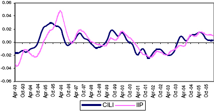
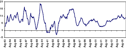
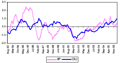
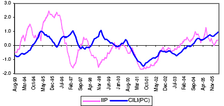


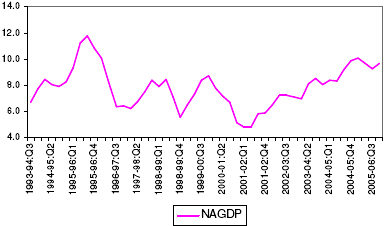

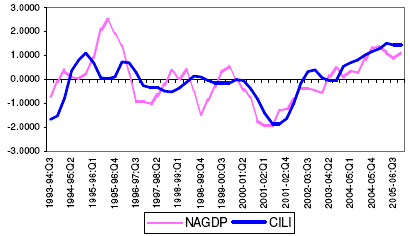

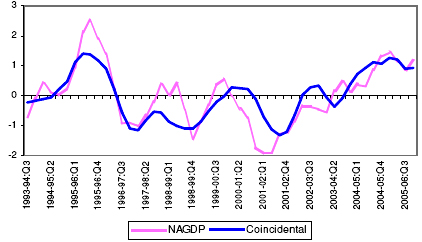
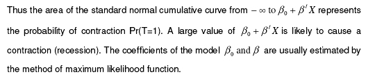

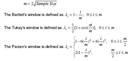
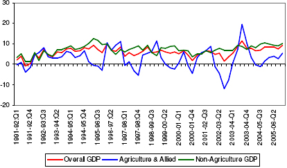

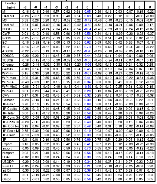

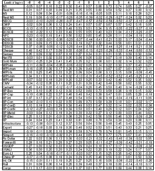

ରିଜର୍ଭ ବ୍ୟାଙ୍କ ଅଫ୍ ଇଣ୍ଡିଆ ମୋବାଇଲ୍ ଆପ୍ଲିକେସନ୍ ଇନଷ୍ଟଲ୍ କରନ୍ତୁ ଏବଂ ଲାଟେଷ୍ଟ ନିଉଜ୍ କୁ ଶୀଘ୍ର ଆକ୍ସେସ୍ ପାଆନ୍ତୁ!
ଆମର ଆପ୍ ଇନଷ୍ଟଲ୍ କରିବାକୁ QR କୋଡ୍ ସ୍କାନ୍ କରନ୍ତୁ


ପେଜ୍ ଅନ୍ତିମ ଅପଡେଟ୍ ହୋଇଛି:


