|
MONETARY POLICY, FOREX MARKETS, AND FEEDBACK UNDER UNCERTAINTY IN AN OPENING ECONOMY
ACKNOWLEDGEMENTS
We thank DRG, RBI for the invitation to work on this project, and valuable inputs to progressing it at various stages. Participants at RBI seminars and an anonymous referee of the DRG series gave useful comments, as did participants of the Money and Finance Conference at IGIDR, where a condensed version was presented. Interactions with RBI officers, during the course of the project, were a source of rich insights and contextual knowledge. We also thank Romar Correa and Sitikantha Pattanaik for comments, Sanchit Arora for excellent research assistance and Reshma Aguiar for secretarial assistance.
Ashima Goyal
EXECUTIVE SUMMARY
We examine options for monetary policy arising from interactions between it and Indian foreign exchange (FX) markets. A brief survey covers recent rapid changes providing a snapshot of current microstructure, and of monetary policy institutions. The survey brings out the growing links between money and FX markets, the sophistication and variety of participants and institutions in markets that are now deep and liquid, and policy trilemmas in dealing with large cross border flows in a rapidly growing emerging market, where fundamentals are uncertain.
Hourly, daily, and monthly data sets for FX markets and policy variables are used to empirically test (i) whether FX market intervention is able to influence levels, returns and volatility, (ii) the influence of microstructure variables, (iii) whether markets anticipate policy, and (iv) the slope of the speculative market demand curve.
There is evidence intervention affects both the level of the exchange rate and its volatility. It has tended to depreciate the exchange rate, in the period of estimation, and reduce its volatility. A broader measure of intervention, derived from the RBI balance sheet, affects levels, while the RBI’s reported measure affects volatility. The results are robust because the estimations use multiple data sets and variable definitions; carefully correct for simultaneity, for properties of the data, and include both policy and market variables. The results support intervention as an additional policy tool.
With respect to microstructure, merchant net demand or order flow affects the level; dealer order flow and turnover variables affect the volatility of exchange rates. Intervention, merchant turnover and order flow increase dealer turnover. So microstructure variables are important. Net demand tends to be more important for levels and turnover for volatility. Merchant turnover is a driving force, perhaps because of the large inflows in the period as noted also in the survey of markets. Volatility and expected volatility increase dealer turnover. So policy should limit volatility.
Signaling becomes a valuable additional instrument as markets deepen and the relative size of intervention falls. Therefore optimal information sharing or signaling is derived in a model of strategic interaction between differentially informed speculators and the Central Bank (CB), adapted to Indian conditions. Shocks affect the information extraction. It turns out that, in the model, to the extent there is greater uncertainty about fundamentals, speculative demand is always well behaved and the CB can optimally reveal more information.
In the empirical tests, anticipated intervention decreases turnover, suggesting it is optimal to reveal information about future intervention. The coefficient of intervention on levels implies the estimated speculative demand curve is downward sloping in the spot rate. So expectations of future exchange rates and intervention are stabilizing and not perverse. A diffuse exchange rate target would contribute to market stability.
Macroeconomic fundamentals represented by interest rate differentials have weak effects on exchange rate levels and volatility but strong effects on FX market turnover. So policy should reduce arbitrage gaps in interest rates. Estimated strategic market behaviour and model derivations both indicate intervention and signaling may be a more effective influence on exchange rates in the Indian context than interest rate changes. The latter should be targeted to the domestic cycle.
Markets form expectations of intervention activity and respond strategically to it. The increase in dealer turnover with intervention may imply strategic intraday arbitrage, whereby dealers profit at the expense of merchants and the CB. More transparency may reduce the scope for such arbitrage.
To the extent behaviour is forward-looking, taking markets into confidence, or strategic revelation of information, can sometimes help achieve policy objectives. But it is also necessary at times to surprise markets (i) since markets can get caught in a trap of self-fulfilling expectations around unsustainable positions, (ii) to reduce build-up of speculative positions. The two ways in which communication makes monetary policy more effective is by creating news or reducing uncertainty. Surprise can be compatible with more transparency if it is linked to random shocks to which the system is subject–then communication enhances news. The markets will then help to bring about the required change, reducing the need for CB action.
Random shock linked two-way movement of the nominal exchange rates will encourage hedging. Guidance to restrain nominal volatility within a diffuse ten percent band around a competitive exchange rate, without committing to specific band edges, makes it possible to maintain export competitiveness, thus helping the real sector.
MONETARY POLICY, FOREX MARKETS, AND FEEDBACK UNDER UNCERTAINTY IN AN OPENING ECONOMY
Ashima Goyal, R. Ayyappan Nair and Amaresh Samantaraya*
1. Introduction
We focus on options for monetary policy arising from the interaction between monetary policy and the Indian foreign exchange (FX) market. Since both markets and the institutions of monetary policy have changed rapidly we survey these changes and provide a snapshot of current microstructure, and institutions. The survey brings out the growing links between money and FX markets, the sophistication and variety of participants and institutions, and policy trilemmas in dealing with large cross border flows in a rapidly growing emerging market, where fundamentals are uncertain.
The literature suggests, on the whole, that moderation of monetary interest rate response is called for under greater uncertainty1. The latter is high in an emerging market slowly moving towards deeper markets and more capital account convertibility. Therefore additional policy instruments maybe required for adequate response to the domestic cycle. The additional instrument we examine is intervention in FX markets, whether such intervention should be announced or secret, and if there is a role for signaling an exchange rate target?
Even if several instruments are used they can be aligned so the markets get a clear signal on the policy stance. For example, when inflation exceeds the target, if a more moderate rise in interest rates is required for the real cycle, intervention to appreciate the exchange rate will work to reduce demand, import costs and inflation and can allow the more moderate interest rate rise2.
Limited volatility in nominal exchange rates around a competitive real exchange rate can contribute to policy objectives of moderating the business cycle while maintaining growth. It reduces the inflationary impact of external price shocks if the nominal exchange rate moves in the opposite direction, for example, an appreciation accompanying a rise in world commodity prices. In addition, limiting volatility reduces entry of noise traders, but some volatility reduces currency risk by encouraging hedging and increasing risk for speculators, thus preventing episodes of high volatility3. Currency risk, and reducing it, is especially important for an opening economy. If the policy is credible and markets respond to signals, intervention requirements are minimized and policy is freed to attend to the domestic cycle. Exchange rate fluctuations have hindered Indian monetary policy response to domestic needs in the recent past.
But it needs to be researched whether such a transparent policy would be supported by the market or serve as an invitation to speculators. In this context we briefly survey the relevant market microstructure literature, and test hypotheses about the role of different participants in Indian FX markets4, impact of central bank (CB) intervention, and strategic interaction with markets.
To the extent behaviour is forward-looking, taking markets into confidence, or strategic revelation of information, can sometimes help achieve policy objectives. But it is also necessary at times to surprise markets (i) since markets can get caught in a trap of self-fulfilling expectations around unsustainable positions (Woodford, 2003), (ii) to prevent the build-up of speculative positions. Blinder et. al (2008) show that the two ways in which communication makes monetary policy more effective is by creating news or reducing uncertainty. But surprise can be compatible with more transparency if it is linked to random shocks to which the system is subject. Then communication enhances news.
Optimal information sharing or signaling is derived in a modified version of the Bhattacharya and Weller (1997) model of strategic interaction between differentially informed speculators and the CB, adapted to Indian conditions. Shocks affect the information extraction. It turns out that, in the model, greater uncertainty about fundamentals makes it more worthwhile for the CB to reveal some information about a target. The result is discussed in the context of the literature on signaling and credibility (Krugman, 1991, Vitale, 2003).
Using hourly, daily, and monthly data sets on FX market rates and turnover, on policy rates and on liquidity provision, we empirically test (i) the extent to which FX market intervention is able to influence levels, returns and volatility, (ii) the influence of microstructure variables, (iii) the extent to which markets anticipate policy, and (iv) the slope of the speculative market demand curve.
We find that intervention affects both the level of the exchange rate and its volatility5. Macroeconomic fundamentals represented by interest rate differentials have weak effects on exchange rate levels and volatility but strong effects on FX market turnover. Microstructure variables are important. Merchant turnover is a driving force, perhaps because of the large inflows in the period as noted also in the survey of markets. Current intervention, volatility and expected volatility increase dealer turnover, but anticipated intervention decreases it, suggesting it is optimal to reveal information about future intervention. The speculative demand curve is downward sloping; expectations are stabilizing and not perverse.
Given this evidence of the impact of policy on markets, intervention and signaling may be a more effective way of influencing exchange rates in the Indian context than interest rate changes. The latter should be targeted to the domestic cycle. Linking exchange rate signals to random supply shocks makes surprise consistent with improved communication. More transparency can reduce speculative positions. Two-way movement within an implicit ten percent band around a competitive exchange rate can encourage hedging while maintaining export competitiveness. A diffuse target is advantageous when speculators are active.
The structure of the study is as follows: Section 2 outlines the development of Indian FX and money markets and consequences for the conduct of monetary policy, empirical tests are reported in Section 3, Section 4 adapts a model of strategic information revelation in FX to Indian conditions, and Section 5 concludes and draws out policy implications.
2. Indian FX and money markets
Intra day trade was first permitted for banks in 1978, but the Indian FX market really grew after liberalization6. The Sodhani Committee (June 1995) gave a comprehensive blueprint for deepening and widening Indian markets. Consequently, wide-ranging reforms were undertaken. An Internal Technical Group on the Foreign Exchange Market (2005) was constituted, to identify areas for further liberalization and to undertake a comprehensive review of measures taken by the Reserve Bank of India (RBI) Some of the recommendations such as freedom to cancel and rebook forward contracts of any tenor, delegation of powers to authorized dealers (ADs) for grant of permission to corporates to hedge their exposure to commodity price risk in the international commodity exchanges/markets and extension of the trading hours of the inter-bank FX market have since been implemented. Tarapore Committee on Fuller Capital Account Convertibility (2006) also made several recommendations for the development of FX markets, interaction of monetary and exchange rate policy and sequencing of capital account liberalization.
These developments in the Indian FX markets are reflected in the increasing trading volume and narrower spreads along with the advent of new instruments for risk management.
2.1 Features of FX Market
Participants
While the core of the FX market is provided by the customers -individuals and corporates who have transactional exposure to the rest of the world, the superstructure comprises ADs, mostly banks who are authorized to deal in FX, brokers who perform the useful role of intermediating mostly between the banks and sometimes between banks and customers and the RBI which is mandated to preserve order in the market. Over the years this aspect of the market has evolved significantly.
- In the past, the customers were mostly passive price takers with emphasis on financing and other banking services relating to foreign trade. In comparison many customer corporates today maintain large treasuries as sophisticated as those of the banks. Most of the customers are well informed not only of exchange rate movements but also of the various hedging tools available.
- While the dominant customers in the past were large exporters and importers, with the advent of capital flows as the prime mover of exchange rate, this role has been usurped by different set of players, viz., Foreign Institutional Investments (FIIs), corporates availing External Commercial Borrowing (ECB), corporates involved in mergers & acquisitions, etc.
- As a natural corollary of this development, the banks, which offer custodial service to the FII have assumed dominance in the interbank forex market.
- With the advent of electronic trading and communication platforms, the role of voice/telephone brokers as intermediaries may be diminishing.
- Since the 1997-98 volatility episodes, the Reserve Bank's preferred
mode of intervention in the market has been through a few public
sector banks largely because of a judgmental view that such an
arrangement would be more effective.
Supply and Demand
The sources of supply and demand for FX have undergone significant changes over the last five years. The current account transactions, which dominated the FX market, have since paved way for capital account transactions as the dominant force behind the exchange rate dynamics. Capital flows in the form of foreign direct investment (FDI), ECB, and FII have all increased manifold over the last few years. The forces behind this transformation are:
- The burgeoning investment demand of a rapidly growing economy has induced the firms to seek overseas markets for resource mobilization.
- The growing clout of India - Moody's upgrade of India to investment grade in March 2007, led to decrease in spread for corporates accessing the overseas capital markets.
- Buoyant corporate profits made investment in Indian equities an attractive proposition and spurred a quantum jump in portfolio inflows. The bright future outlook has also motivated significant increase in foreign direct investment as well as investment by private equity funds. The pullout of about $13 billion by portfolio flows in 2008 as a consequence of the financial crisis, remains small compared to past inflows.
- Indian entrepreneurship proudly announced its arrival in the global corporate arena with a spate of large acquisitions.
- The large and increasing deficit on the merchandise account has been substantially offset by concomitant increase in service exports and remittance by the Indian diaspora leaving the field to autonomous capital flows as a major factor influencing the exchange rate.
FX Turnover
The Indian FX market has grown manifold over the last several years. The average daily turnover, which was in the vicinity of US $ 3.0 billion in 1998-99 grew to US $ 18 billion during 2005-06. The turnover rose considerably to US $ 48 billion during 2007-08 with the monthly turnover crossing US $ 65 billion in February 2007. The inter-bank to merchant turnover ratio halved from 5.2 during 1997-98 to 2.3 during 2007-08 reflecting the growing participation in the merchant segment of the foreign exchange market. The spot market remains the most important FX market segment accounting for 51 per cent of the total turnover. Its share has declined marginally in recent years due to a pick up in the turnover in derivative segment. Even so, Indian derivative trading remains a small fraction of that in other developing countries such as Mexico or South Korea. Short-term instruments with maturities of less than one year dominate, and activity is concentrated among a few banks (IMF 2008).
Products
FX market is a dynamic environment that is constantly innovating and evolving. Along with the spot and forwards market, the derivative segment also plays a significant role. Derivatives help in price discovery and enable market participants to manage risk by hedging their underlying exposure. Banks in India have been increasingly using derivatives for managing risks and have also been offering these products to corporates. In India, various informal forms of derivatives contracts have existed for a long time. Cross-currency derivatives with the rupee as one leg were introduced with some restrictions in April 1997. Rupee-foreign exchange options were allowed in July 2003. The foreign exchange derivative products are now available in Indian financial markets can be grouped into four broad segments, viz., forwards, options (foreign currency rupee options and cross currency options), currency swaps (foreign currency rupee swaps and cross currency swaps), and exchange traded currency futures.
Available data indicate that the most widely used derivative instruments are the forwards and foreign exchange swaps (rupee-dollar).Options have also been in use in the market for the last four years. However, their volumes are not significant and bid-offer spreads are quite wide, indicating that the market is relatively illiquid. Going forward, one of the key challenges will be to revive this market as the implied volatility inherent in option prices can act as a key input in risk management strategies and also in policy decisions. The development of currency futures as a hedging instrument has received growing attention, although at present in India, as elsewhere, FX transactions are mostly over-the-counter structured by banks. But there is a user demand for liquid and transparent exchange traded hedging products. They are also easier to regulate. An offshore Indian Rupee futures exchange started with the Dubai Gold and Commodities Exchange starting operations in June 2007. Indian stock exchanges also set up futures exchanges in 2008. The nondeliverable forward (NDF) market has been growing but still accounts for only about a quarter of onshore trading. Such markets create problems for policy. It is international experience that they wither away as domestic markets deepen and offer all facilities.
Regarding the forward market in India, it is fairly liquid up to one year. The price movement in the near-term bucket is a reflection of rupee liquidity in the interbank market and overnight interest rates whereas the six-month and one-year rates are determined not only by where liquidity is today but where it is expected to be in the future. Importers and exporters also influence the forward markets and it is observed that forward rates in a particular segment may not be in alignment with other segments due to the excess supply/demand from importers/exporters in that segment. Further, with the gradual opening up of the capital account, the forward premia is getting aligned with interest rate differential.
In respect of forward contracts and swaps, which are relatively more popular instruments in the Indian derivatives market, cancellation and rebooking of forward contracts and swaps in India have been regulated. The objective has been to ensure that excessive cancellation and rebooking do not add to the volatility of the rupee. Gradually, however, the Reserve Bank has been taking measures towards eliminating such regulations.
FX Risk Management
There has been a significant improvement in market infrastructure in terms of availability of trading platforms and settlement mechanisms. Several emerging markets in recent years have implemented domestic real time gross settlement (RTGS) systems for the settlement of high value and time critical payments in the domestic leg of foreign exchange transactions. Apart from risk reduction, these initiatives enable participants to actively manage the time at which they irrevocably pay away when selling the domestic currency, and reconcile final receipt when purchasing the domestic currency. Recognizing the systemic impact of foreign exchange settlement risk, an important element in the infrastructure for the efficient functioning of the Indian foreign exchange market has been the clearing and settlement of inter-bank USD-INR transactions.
Following the recommendations of the Sodhani Committee, the Reserve Bank had set up the Clearing Corporation of India Ltd. (CCIL) in 2001 to mitigate risks in the Indian financial markets. The CCIL commenced settlement of foreign exchange operations for inter-bank USD-INR spot and forward trades from November 8, 2002 and for interbank USD-INR cash and tom (tomorrow) trades from February 5, 2004. The CCIL now settles 90-95 percent of interbank rupee-dollar transactions. It undertakes settlement of foreign exchange trades on a multilateral net basis through a process of novation. All spot, cash and tom transactions are guaranteed for settlement from the trade date. Further, the guaranteed settlement of transactions by the CCIL has been extended to all forward trades as well. Apart from managing foreign exchange settlement risk, participants also need to manage market risk, liquidity risk, credit risk and operational risk. The Reserve Bank has framed guidelines for banks to manage their inter-bank foreign exchange dealings and exposures to derivative markets which include the limit on net overnight open exchange position and aggregate gap limits.
A conviction of possible two-way movement of the exchange rate, large enough to deliver a substantial loss to one-way bets is, however, a pre-requisite for hedging or the laying off of currency exposure. Despite deepening FX markets, the moderate two-way movement within an implicit 5 percent band seen over 2004-06 was not sufficient to overcome strong expectations of medium term appreciation given India's high growth rate. In 2007, market expectations of the Rupee-USD rate had even reached 32. Many corporates borrowed abroad based on such expectations, increasing currency risk. Some had entered into so called hedging deals, which were actually bets on the value of the Swiss Franc. With the volatility in currency markets and steep rupee depreciation in 2008 many firms lost money. Many such deals, where Indian banks were often a front for foreign banks, sidestepped existing rules that prevented leverage or underlying risk that exceeded export income. Although firms were not allowed to write options deals were structured so that in effect firms were writing options. The deals were so complex that firms sometimes did not understand what the risks they were taking. Thus availability of more instruments alone only makes leveraged speculation or bets on future currency value possible. Establishing inducement to hedge through sufficient flexibility of the exchange rate is more important. So are transparency, clarity and information
2.2 Money market developments
Substantial developments in the Indian money market include newer instruments, broader participation, building of market infrastructure, and strengthening of prudential practices. The liquidity adjustment facility (LAF), made operational in June 2000, provides standing facilities to curb short-term volatility in liquidity conditions. Daily open market operations (OMOs) smooth and guide short interest rates. Liquidity is injected by accepting repo7 bids, with an overnight maturity, from banks and primary dealers, while it is absorbed through the acceptance of reverse repo bids. Liquidity operations are conducted regularly by means of daily tenders under a uniform price auction. The repo and the reverse repo rates are two policy rates specified for lending and borrowing of funds. Liquidity conditions are influenced either by rejecting bids or by changing the LAF rates, at discrete intervals. The overall quantity to be absorbed/injected is determined from the RBI's assessment of the banking system's liquidity requirements. Additional liquidity is made available to banks through the standing facility of export credit refinance. The RBI also conducts longer-term repo auctions at a fixed rate or at variable rates depending on market conditions. It has moved to more active liquidity management, with frequent OMOs, but more medium-term instruments such as government securities with 1-2 week maturities are required for fine-tuning (IMF, 2008). In the period of large capital flows, the LAF was largely used to absorb liquidity.
Developments in institutional and technological infrastructure such as the introduction of screen-based dealing system and growth of the collateralized segment have also provided avenues for better liquidity and risk management. With the Collateralized Borrowing and Lending Obligations (CBLO) repo instrument developed by CCIL for its members, the volume in the collateralized segment of the overnight inter-bank deposit market has overtaken that of the uncollateralized one.
2.3 Linkages among Markets and Policy Responses
The introduction of such reform measures has strengthened the inter-linkage between forex markets and other segments of the market viz., money market, Government securities market and capital market. The linkages between forex markets and domestic markets has been so close that any policy measure taken with respect to one market is immediately reflected in the form of price action in the other market. Further, these linkages to a large extent depend on the foreign currency liabilities and assets banks can maintain and the extent and degree to which they can be converted to rupees and vice versa. Banks use the FX swaps route to manage their rupee liquidity depending upon surplus/shortage of the same. The popularity of FX swaps reflect that banks and others in the FX market often find it easy to shift from foreign currency to rupee or vice versa without incurring exchange rate risk of holding an open position or exposure in the currency that is temporarily held. Swaps and options are essentially inter-bank transactions, and account for about 50 percent of CCIL trade settlement (IMF, 2008).
The integration of FX markets with other domestic markets requires co-ordination of monetary and exchange rate policy. For instance, the growing importance of capital inflows in determining exchange rate movements as against trade flows has forced the Reserve Bank to attempt to manage these flows effectively so they have little impact on the domestic monetary policy. Changes in the policy rates through its immediate impact on domestic interest rates can affect the exchange rate and in turn the real economy. It also impacts volatile arbitraging capital flows, in response to interest differentials, as markets are now highly integrated.
2.4 Monetary Policy
One of the key challenges facing India and other emerging market economies (EMEs) is the dilemma in grappling with the inherently volatile increasing capital flows relative to domestic absorptive capacity. Consequently, the reconciliation of fixed or managed exchange rates, open capital accounts and discretion in monetary policy has to be managed in a 'fuzzy' manner rather than satisfactorily resolved - a problem that gets exacerbated due to huge uncertainties in global financial markets and possible consequences in the real sector.
This absorption by CBs reflects two key policy concerns. First, drawing from EMEs experiences with financial crises, reserve accretion reflects attempts to build-up reserves to be able to meet unpredictable and temporary imbalances in international payments and thereby, provide confidence to financial markets. Second, it reflects concerns with the large appreciation in the exchange rate that would have occurred, had these inflows not been absorbed by the monetary authorities.
However, when excess inflows tend to be persistent, market purchases by the central bank to support the exchange rate, expand base money and, over time, fuel inflationary pressures. Higher inflation could offset the gains obtained from avoiding nominal appreciation. The monetary authorities, therefore, attempt to avoid exchange rate appreciation and, at the same time, control domestic money supply through sterilization, i.e., sales of government or central bank securities against purchases of foreign securities. Apart from sterilization in the form of open market operations, another key instrument of sterilization, at least in the emerging context, is the control over cash reserve ratios. Other instruments of sterilization include: shifting of public sector and government deposits from the commercial banks to the central bank; foreign exchange swaps; fiscal tightening; liberalization of trade policies and capital outflows; and finally, a greater degree of flexibility in the exchange rate. Thus a mix of quantitative and market-based instruments is used to carry out sterilization objectives.
Like other EMEs, India too has faced unprecedented surges in capital flows in recent years. In the period since October 1995, capital flows gathered pace, notwithstanding brief episodes of reversals. They created problems for monetary management. During 2007-08 net inflows leapt to US $ 109.6 billion as compared to US $ 46.4 in the previous year. As a response to this, the Reserve Bank of India has been broadly following the same strategy of absorbing excess inflows in to its foreign exchange reserves while also permitting movements in the exchange rate of the rupee consistent with underlying fundamentals. The period since 1996 has also seen efforts by the Reserve Bank to increase the stock of marketable debt with it through conversion of the special securities. A number of other steps were taken such as further liberalization of the capital account, pre-payment of external debt, tightening of interest rate ceilings for non-resident deposits and greater exchange rate flexibility.
These efforts were, however, unable to absorb the market surplus and sterilization operations remained the key policy instrument of monetary management. But by 2003-04, the stock of government debt securities was nearing depletion. Thus, in contrast to the constraints from absence of marketable securities (albeit non-marketable securities were relatively large) in the initial stages of capital flows during 1993-94, 2003-04 onwards saw a threat to viability of sterilization emerging from the fast depleting stock of government securities. In addition, quasi-fiscal costs would have undermined the Reserve Bank's profitability and strength of its balance sheet.
Against this backdrop, the Market Stabilization Scheme (MSS) (consisting of 91-day to 1-year government bonds) was introduced in March 2004 to enable sterilization operations by the Reserve Bank and to absorb the interest costs in a transparent manner. While these issuances do not provide budgetary support, interest costs are borne by the government. As far as government securities market is concerned, MSS securities are also traded in the secondary market, at par with the other government stock. By explicitly showing the sterilization costs in the Budget, this process ensures a healthy debate on the costs and the benefits of sterilization. Moreover, in the post-reform period, the medium term policy was to gradually reduce CRR to its statutory minimum. But, in response to unprecedented surge in foreign capital inflows, CRR was reactivated since December 2006 as a monetary policy instrument in the sterilization process also. Sterilization measures such as increase in CRR and MSS had to be reversed under outflows as reserves fell by more than 50 billion dollars and RBI dollar sales sucked out liquidity, during the 2008 global financial crisis.
2.5 Looking Ahead
Exchange Rate Flexibility and Hedging
The Reserve Bank continues with careful monitoring and management of exchange rates with flexibility, without a fixed or pre-announced target or band while intervening to reduce excess volatility, smoothen the exchange rate movement, and prevent emergence of destabilizing speculative activities. Two-way exchange rate movement creates an incentive for hedging, although movement in excess of ten percent is required to sufficiently raise the risk to bets on an expected future value.
Banks are expected to educate customers and encourage them to use appropriate hedging instruments and strategies to cushion against possible adverse exchange rate movements, but it may be necessary to consult experts, in addition to interested parties selling derivatives. The Reserve Bank has been gradually expanding the range of instruments available for hedging. Exchange traded derivatives such as futures have the advantage of transparency, standardization, and reduced counterparty risk.
Net Overnight Open Position Limit (NOPL) and Aggregate Gap Limit (AGL)
Fixing of NOPL and AGL limits by the Reserve Bank is a legacy of the past where the FERA regime mandated RBI to conserve foreign exchange. In today's liberalized atmosphere where the banks have been given sufficient operational freedom, it may not be desirable for RBI to micromanage the operation of banks. Therefore, time may be appropriate to allow banks to fix their own NOPL and AGL limits based on their risk appetite and ability to manage the exposure. But prudential regulation and supervision must, of course, be adequate to cover systemic risk and prevent excessive leverage.
Capital Account Convertibility
The gradual opening up of capital account has been marked by increase in volatility in exchange rate and interest rate. In such a scenario, new hedging tools can allow economic agents to lay off specific types of risk. The Reserve Bank is working on various fronts in this regard, including a well-developed rupee futures market, and removing the operational impediments to liberalization.
Economic Exposure
Historically, the availability of hedging tools against foreign exchange risk has been limited to entities with direct underlying foreign exchange exposures. The insistence on this requirement of underlying exposure is motivated by the apprehension that a sparsely populated and shallow market can be manipulated by a few large players with a view and resources to back it. Besides, only those entities with an exposure to international markets faced foreign exchange risk. In the present atmosphere of increasing integration with the global economy, foreign exchange risk confronts a larger set of economic agents and it is perhaps necessary to anchor policy decisions on the concept of "economic exposure", which refers to the effect of exchange rates on a firm's value. Any firm not in export/import business but with an economic exposure to fluctuations in exchange rates (because either its raw materials or its products may be substitutes or complements of exported/ imported items) is affected by the movements in the exchange rates and therefore has to be enabled to hedge its exposures.
The Reserve Bank has taken gradual steps to enable corporates greater flexibility to manage their exposures. The Annual Policy Statement for 2007-08 announced a host of measures to expand the range of hedging tools available to market participants as also facilitate dynamic hedging by residents. To hedge economic exposures, it has been proposed that ADs (Category- I) may permit (a) domestic producers/users to hedge their price risk on aluminum, copper, lead, nickel and zinc in international commodity exchanges, based on their underlying economic exposures; and (b) actual users of aviation turbine fuel (ATF) to hedge their economic exposures in the international commodity exchanges based on their domestic purchases. In order to facilitate dynamic hedging of foreign exchange exposures of exporters and importers of goods and services, it has been proposed that forward contracts booked in excess of 75 per cent of the eligible limits have to be on a deliverable basis and cannot be cancelled as against the existing limit of 50 per cent. In order to give greater flexibility to corporates with overseas direct investments, cancelling and rebooking of forward contracts for hedging overseas direct investments is allowed. To enable small and medium enterprises to hedge their foreign exchange exposures, it has been proposed to permit them to book forward contracts without underlying exposures or past records of exports and imports. Further, to enable resident individuals to manage/hedge their foreign exchange exposures, it has been proposed to permit them to book forward contracts without production of underlying documents up to an annual limit of US $ 100,000, which can be freely cancelled and rebooked.
Structure and International Developments
FX markets have special features8. They are the most liquid markets with daily market turnover at $ 3.2 trillion (BIS 2007). But since they are decentralized they are fragmented and less transparent. There is no incentive to share information on order flows. The majority of transactions is bilateral and occurs in opaque markets without a physical market place. Although new technologies are causing change, these special features continue to dominate. Electronic systems such as Electronic Broking System (EBS) or Reuters D3000, established in 1993, account for 85 percent of interbank trading. They provide ex ante anonymous limit order bid ask pricing to dealers. Although voice trading dominates in customer trades, electronic portals are being introduced here also. Electronic systems allow netting, lower settlement and counterparty risk, have operational benefits such as reducing human error and have driven a large increase in liquidity. But they do not increase the transparency of the foreign exchange market since system governing boards treat electronic order flow as strictly confidential. Therefore information on order flow remains sectoral. Trades are initiated based on macro data and differential order flow information, with the aim of rebalancing portfolios.
Participants are heterogeneous with diverse information sets and reaction speeds, so that market efficiency does not hold and profit opportunities persist for informed traders. Central banks have a dominant position. Although the interdealer market continues to account for the majority of transactions (59%) this share has decreased through the nineties because of the growth of large financial customer groups such as hedge funds. Corporate treasuries have also become sophisticated. Sudden shifts in positioning by large hedge funds that have the fastest reaction speeds and operate with high leverage can magnify shocks to FX markets. They implement currency programs to secure a notional capital value that may be a benchmark risk free rate. Despite such activity currency markets remained largely stable during the financial crisis of 2008, partly because risk management procedures had been improved after the LTCM crisis. Banks impose position limits for individual traders, and risk capital made available is a function of past performance. Incentives to take risk are reduced because losses reduce the trader's risk capital while profits are shared with the bank (Geithner, 2004).
3. Empirical Tests
3.1 Variables and Data
Variable definitions are given in Table 1. Apart from exchange rate return and volatility variables, there are policy and market variables. Policy variables include intervention in FX markets, policy rates and dummies. Since intervention data is not available at the daily frequency, lafps is used as a proxy. Daily liquidity absorption generally rises when intervention is releasing rupees into the market9. Apart from intervention to reduce volatility the RBI has also been accumulating foreign exchange reserves in the face of large inflows of foreign capital. Weekly data on foreign exchange assets is available so that monthly change in foreign exchange assets held by the RBI is derived as fxach, an alternative measure of intervention10. The basic variables listed are further transformed in regressions as necessary, to take care of properties of the data generating process at different frequencies. Rules are followed in naming these transformations. For example, ch at the beginning of a variable denotes the first difference; sq at the beginning of a variable denotes the squared value.
Table 1: Variables |
Variables |
Definition |
chloge |
log of exchange rate (e) at 5:30 pm (INR/USD) day t+1 minus log e at t |
cmr |
call money rate, (i) average daily (ii) monthly as average of daily cmr |
err |
Cash reserve ration |
| dealerratio |
dturn/totturn |
dps |
interbank purchase minus sale of USD (millions) in spot and forward markets (excluding swap and forward cancellation) |
dturn |
interbank purchase and sale of USD (m) in spot, forward, and swap markets |
dvcmr |
takes value 1 from March 20, 2007 to August 17, 2007 |
dvgr |
takes value 1 from December 26, 2006 to May 2008 |
dvexpec |
takes value 1 for two days prior to intervention days |
dvintv |
takes value 1 for days when RBI was intervening in FX markets |
echav |
log difference of (i) daily RBI reference exchange rates, (ii) monthly average e |
egarch11 |
egarch (1,1) volatility for monthly exchange rate including two AR terms |
eegarch1 |
egarch (1,6) volatility measure for daily exchange rate |
esd |
standard deviation of exchange rates derived from average of (i) daily rates for the monthly data set (ii) hourly quotes from the reuters 3 month data set for daily data set |
fxach |
change in foreign exchange assets held by RBI (monthly) |
idiff |
call money rate minus US federal fund rate (ffr) |
intvnet |
net purchase (+) minus sales (-) of USD (m) |
lafps |
purchase minus sale in repo/ reverse repo auctions in LAF, that is, net injection (+) minus net absorption (-) of liquidity by RBI |
mps |
purchase minus sale of USD (m), by merchants in spot and forward markets (excluding swap and forward cancellation) |
mturn |
purchase and sale of USD (m), by merchants in spot, forward and swap markets |
r |
repo rate or rate at which RBI lends in the LAF |
rr |
reverse repo rate or rate at which RBI absorbs liquidity in the LAF |
totps |
total purchase minus sale of USD (m) spot and forward, excluding swap and forward cancellation (purchase + , sale -) |
totturn |
total spot, forward, swap, purchase and sale of USD (m), interbank and merchant |
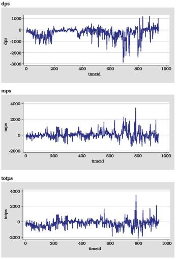
In FX market variables, total dollar net demand, totps, is also broken up into dealer or interbank net demand, and that originating with customers or "merchants" as it is called in the data set. These dealer and customer demands are the order flow variables used in FX market microstructure studies. Since we are interested in analyzing total market transactions, we also calculate total turnover, totturn, which is similarly broken up into transactions due to dealers and transactions due to customers.
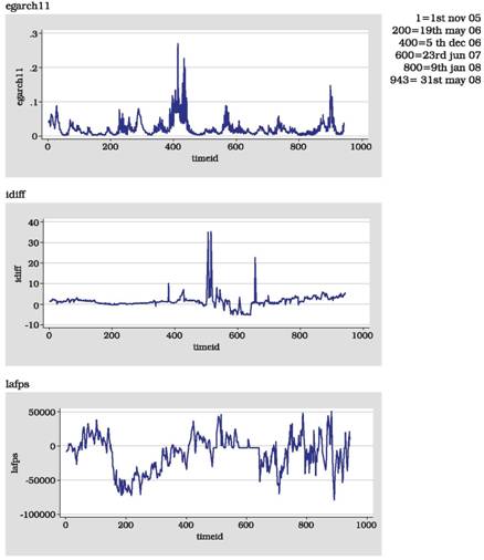
After a series of reforms starting in the late nineties, foreign exchange markets had acquired a degree of depth by 2002; money markets also changed with the starting of the liquidity adjustment facility or LAF around this time, as we saw in the preceding section. Therefore our monthly data set starts in 2002 and continues to May 2008. Since all the required series were not available in the early years, the daily data set runs from November 2005 to May 2008. The source for these two data sets is the RBI database. A third data set from Reuters gives hourly changes in the exchange rate over the period September-November 2007.
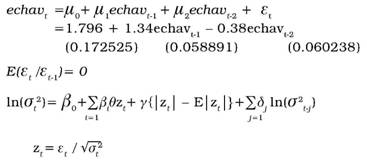
Separate Garch models at the daily and hourly frequency provide a measure of exchange rate volatility. A number of Garch models were estimated by maximizing the log-likelihood through an iterative process. The best were selected based on diagnostics such as AIC, F-tests, and the Q test. The latter checks the null hypothesis that there is no remaining residual autocorrelation, for a number of lags, against the alternative that at least one of the autocorrelations is nonzero. The null is rejected for large values of Q. The best fitting equations are given below. Standard error is in ( ), p-value in [].
Monthly [egarch(1,1)]
 |
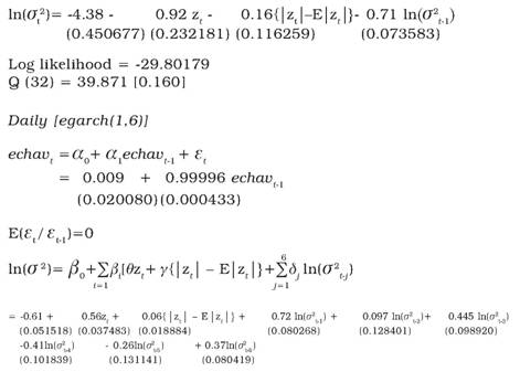 |
Log likelihood = 1677.307 Q (36) = 29.760 [0.759]
The simple standard deviation (esd) of daily exchange rates was also used as a volatility measure at the monthly frequency. Since hourly exchange rates were only available for a limited three-month data set, esd for daily exchange rates could only be calculated for this limited period.
3.2 Analysis of data
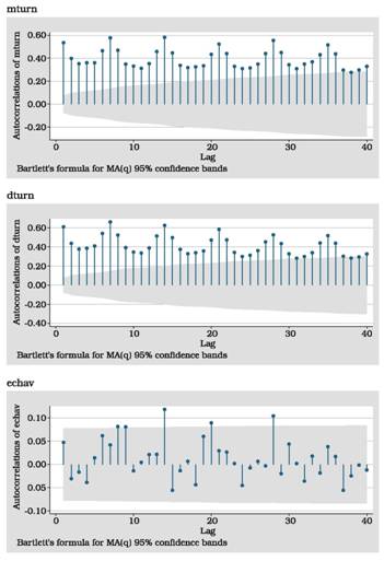
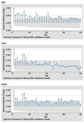
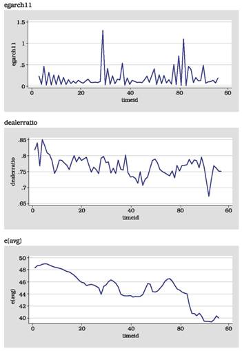
Sample statistics for key variables from monthly and daily data are presented in Tables 2 and 3 respectively, and graphs against time and the autocorrelation functions after that. Three period autocorrelation coefficients were derived using the model Y(t)=a+bY(t-1)+cY(t-2)+dY(t-3)+e(t).
The sample statistics (Tables 2, 4) show since skew is not zero, kurtosis is far from 3 and first order autocorrelation especially is high and significant, the distributions are far from normal. Cross correlations between market
Table 2: Daily Sample Statistics |
|
Mean |
Kurtosis |
Skewness |
SD |
p1 |
p2 |
p3 |
eegarch1 |
0.02 |
25.49 |
3.86 |
0.27 |
0.20 |
-0.007 |
0.58 |
|
|
|
|
|
(0.000) |
(0.881) |
(0.000) |
idiff |
1.42 |
51.69 |
5.09 |
3.21 |
0.99 |
-0.33 |
0.10 |
|
|
|
|
|
(0.000) |
(0.000) |
(0.270) |
lafps |
-11961.97 |
2.65 |
-0.41 |
25481.78 |
0.71 |
0.22 |
-0.058 |
|
|
|
|
|
(0.000) |
(0.030) |
(0.519) |
mturn |
4806.05 |
3.33 |
0.70 |
2530.62 |
0.40 |
0.29 |
0.16 |
|
|
|
|
|
(0.000) |
(0.000) |
(0.017) |
dturn |
14974.33 |
2.82 |
0.13 |
7697.9 |
0.52 |
0.18 |
0.15 |
|
|
|
|
|
(0.000) |
(0.016) |
(0.020) |
dps |
-261.16 |
7.80 |
-1.64 |
483.18 |
0.47 |
0.06 |
0.24 |
|
|
|
|
|
(0.000 |
(0.394) |
(0.001) |
mps |
54.49 |
7.74 |
1.18 |
520.05 |
0.48 |
-0.01 |
0.15 |
|
|
|
|
|
(0.000) |
(0.855) |
(0.026) |
totps |
-206.23 |
7.93 |
0.72 |
526.04 |
0.41 |
0.23 |
0.03 |
|
|
|
|
|
(0.000) |
(0.008) |
(0.697) |
Note: p-values, which give the level of significance, are in brackets |
daily/monthly
Table 3: Correlations with echav |
|
echav |
idiff |
dps |
mps |
totturn |
intvnet |
echav |
|
0.17 |
0.18 |
-0.57 |
-0.10 |
-0.26 |
idiff |
-0.03 |
|
0.56 |
-0.22 |
-0.70 |
-0.47 |
dps |
0.15 |
0.14 |
|
-0.39 |
-0.55 |
-0.66 |
mps |
-0.15 |
-0.08 |
-0.45 |
|
0.11 |
0.57 |
totturn |
0.03 |
0.19 |
-0.19 |
-0.13 |
|
0.57 |
lafps |
-0.10 |
0.30 |
-0.04 |
-0.03 |
0.22 |
|
Note: The lower panel reports correlations between the order flows at the daily frequency and the upper panel reports the monthly frequency. In the monthly frequency lafps is replaced by intvnet. |
Table 4: Monthly Sample Statistics |
|
Mean |
Kurtosis |
Skewness |
SD |
p1 |
p2 |
p3 |
dturn |
197523.6 |
3.39 |
1.22 |
131885.6 |
0.65 |
-0.05 |
0.42 |
|
|
|
|
|
(0.000) |
(0.717) |
(0.001) |
idiff |
2.42 |
5.27 |
-0.65 |
2.04 |
0.52 |
0.24 |
0.01 |
|
|
|
|
|
(0.000) |
(0.070) |
(0.919) |
intvnet |
2927.61 |
5.41 |
1.23 |
3521.93 |
0.11 |
0.18 |
0.38 |
|
|
|
|
|
(0.455) |
(0.194) |
(0.026) |
mturn |
61707.08 |
3.86 |
1.30 |
44141.98 |
0.57 |
0.36 |
0.08 |
|
|
|
|
|
(0.000) |
(0.011) |
(0.512) |
esd |
0.20 |
5.94 |
1.72 |
0.18 |
0.26 |
0.06 |
0.00090 |
|
|
|
|
|
(0.060) |
(0.657) |
(0.994) |
egarch11 |
0.19 |
2.94 |
13.29 |
0.22 |
-0.20 |
3472763 |
0.0099 |
|
|
|
|
|
(0.1211) |
(0.1162 ) |
(0.1211) |
echav |
-0.0011 |
5.42 |
-0.61 |
0.0050 |
0.37 |
-0.05 |
-0.07 |
|
|
|
|
|
(0.004) |
(0.714) |
(0.714) |
dps |
-2697.37 |
6.18 |
-1.89 |
4669.93 |
0.55 |
0.17 |
-0.06 |
|
|
|
|
|
(0.000) |
(0.216) |
(0.630) |
mps |
1366.86 |
3.70 |
0.39 |
3530.25 |
0.25 |
-0.03 |
0.36 |
|
|
|
|
|
(0.027) |
(0.791) |
(0.002) |
totps |
-1330.52 |
4.08 |
-1.36 |
4559.46 |
0.51 |
0.34 |
-0.12 |
|
|
|
|
|
(0.000) |
(0.009) |
(0.298) |
Note: p-values in brackets. |
and policy variables (Tables 3, 5) are higher at the monthly (upper triangle) compared to the daily frequency. This follows: the level of simultaneity should be higher as more information is shared with passing time.
Volatility variables (Table 5) show a high correlation between dturn and mturn. Monthly intvnet is strongly correlated with market variables, and all these variables are strongly correlated with idiff. Table 3 with echav shows idiff to be strongly correlated with lafps, dps, totturn, intvnet; dps is strongly correlated with mps and totturn, mps with echav, while monthly intvnet is strongly correlated with idiff and market variables.
The strong cross-correlations suggest that some instrument variable technique would be required to extract information on the effectiveness of intervention and market interactions. The non-normality of the distributions implies that GMM estimation is required.
Table 5: Correlations with the Volatility Variable |
|
egarch11 |
idiff |
intvnet |
mturn |
dturn |
mps |
dps |
eegarch1 |
|
-0.08 |
0.14 |
0.04 |
0.08 |
0.11 |
-0.04 |
idiff |
0.045 |
|
-0.47 |
-0.67 |
-0.70 |
-0.20 |
0.56 |
lafps |
0.12 |
0.30 |
|
0.55 |
0.57 |
0.57 |
-0.66 |
mturn |
-0.15 |
0.22 |
0.19 |
|
0.97 |
0.06 |
-0.50 |
dturn |
-0.15 |
0.18 |
0.22 |
0.84 |
|
0.11 |
-0.56 |
mps |
-0.03 |
-0.08 |
-0.03 |
0.08 |
0.14 |
|
-0.38 |
dps |
0.13 |
0.14 |
-0.04 |
-0.05 |
-0.23 |
-0.45 |
|
Note: The lower panel reports correlations between the order flows at the daily frequency and the upper panel reports the monthly frequency. In the monthly frequency eegarch1 is replaced by egarch11 and lafps is replaced by intvnet. |
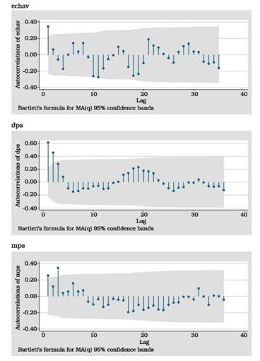
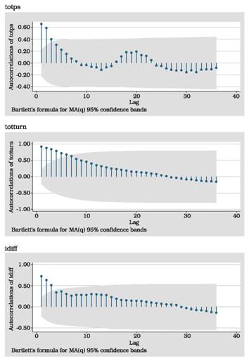
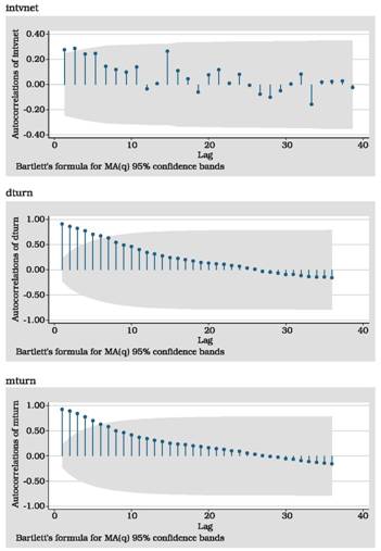
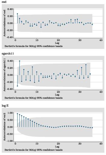
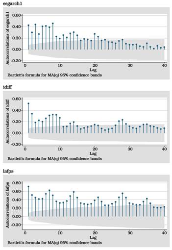
The graphs of the auto-correlation function (Appendix Charts 1 and 2) show autocorrelation, but this does not lie outside the confidence bands except for daily mturn and dturn implying that these variables should be first differenced.
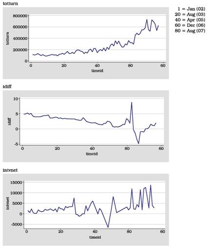
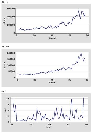
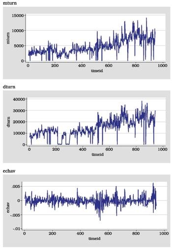
The graphs of the variables (Appendix Charts 3 and 4) show larger fluctuations and/or trend growth in the later period suggesting the use of the dummy variable dvgr, which takes the value of unity from December 1, 2006, to capture market deepening. There is also an outlier in the sharp fluctuations in call money rates coinciding with the period March 5, 2007 to August 6, 2007, when limits were placed on LAF reverse repo (absorption of liquidity) at Rs. 3,000 crores. The variable dvcmr is to take care of this. The last two graphs of Chart set 4 show that a rise in the dealer share in the turnover is not associated with large changes in the exchange rate. During the period of the greatest changes the dealerratio was flat. The graphs do not show any seasonality.
The graphs suggest a possible unit root in monthly mturn dturn toturn, which was confirmed by formal tests. Unit root tests were conducted using the Phillips Perron test (result available on request). All variables were stationary except monthly mturn dturn and toturn. Therefore first differences of these variables were used.
Granger causality analysis done with two sets of stationary variables at the daily and monthly frequency (Tables 6 and 7) show evidence of simultaneous causation between market and policy variables. Policy variables idiff and intvnet affect market variables, which affect the exchange rate and its volatility. Policy variables also directly affect volatility. Market variables have more feedback on policy at the monthly frequency implying that policy reacts with a lag. The order flow variables, mps and dps are not exogenous as in the market microstructure literature, implying that simultaneity handling techniques such as GMM are required (Table 7).
Table 6: Granger Causality for Exchange Rate |
Monthly |
Daily |
Causality from |
to |
Causality from |
to |
chtotturn (0.0033) |
idiff |
echav (0.0042) |
idiff |
dps (0.0213) |
totturn (0.0348) |
echav (0.0984) |
|
intvnet (0.1089) |
dps (0.0224) |
mps |
|
|
totturn (0.0776) |
echav (0.0335) |
mps |
lafps (0.2213) |
|
|
idiff (0.2526) |
echav (0.0038) |
dps |
|
|
chtotturn (0.0829) |
idiff (0.0001) |
dps |
|
|
mps (0.0782) |
dps (0.1253) |
chtotturn |
|
|
echav (0.1513) |
dps (0.0477) |
totturn |
|
|
lafps (0.0635) |
echav (0.0432) |
intvnet |
|
|
chtotturn (0.0494) |
mps (0.0501) |
lafps |
idiff (0.2366) |
totturn (0.1946) |
dps (0.2761) |
idiff (0.2718) |
chtotturn (0.1758) |
echav |
dps (0.2747) |
echav |
Note: Based on VAR Monthly- idiff mps dps chtotturn intvnet echav; VAR Daily- idiff mps dps totturn lafps echav; p values shown in brackets. The coefficients are in ascending order. Variables with p- values exceeding 0.3 are not reported |
Table 7: Granger Causality for Exchange Rate Volatility |
Monthly (egarch 11) |
Monthly (esd) |
Daily |
Causality from |
to |
Causality from |
to |
Causality from |
to |
chdturn (0.000) |
idiff |
chmturn (0.0905) |
idiff |
mps (0.0500) |
idiff |
intvnet (0.0010) |
esd (0.1500) |
mturn (0.0941) |
chmturn (0.0029) |
chdturn (0.1594) |
|
|
egarch 11 (0.0188) |
mps (0.2083) |
|
|
chdturn (0.000) |
chmturn |
|
|
dturn (0.0001) |
mturn |
mps (0.0002) |
mps (0.0196) |
intvnet (0.0237) |
eegarch1 (0.2601) |
idiff (0.1711) |
|
|
|
|
|
chdturn (0.0086) |
mps |
idiff (0.0444) |
mps |
|
|
chmturn (0.0785) |
chmturn (0.0591) |
|
|
intvnet (0.1043) |
esd (0.1637) |
idiff (0.1533) |
mps |
idiff (0.1293) |
chdturn (0.2287) |
|
|
intvnet (0.2686) |
|
|
idiff (0.0001) |
intvnet |
idiff (0.0283) |
intvnet |
|
|
chdturn (0.0064) |
chdturn (0.0809) |
mps (0.0265) |
lafps |
egarch 11 (0.0998) |
esd (0.2015) |
mturn (0.2236) |
mps (0.0625) |
chdturn |
|
|
lafps (0.0466) |
dturn |
chmturn (0.0832) |
|
|
eegarch1 (0.0545) |
intvnet (0.0963) |
chmturn (0.3047) |
chdturn |
mturn (0.1257) |
idiff (0.1216) |
|
|
mps (0.2868) |
intvnet (0.1533) |
egarch11 |
|
|
lafps (0.2092) |
eegarch1 |
idiff (0.2027) |
chdturn (0.0385) |
esd |
dturn (0.2488) |
chmturn (0.2766) |
intvnet (0.2191) |
idiff (0.2720) |
Note: Based on VAR monthly- idiff chmturn mps intvnet chdturn egarch11; idiff chmturn mps intvnet chdturn esd; VAR daily- idiff mturn mps lafps dturn eegarch1; p values shown in brackets with the coefficients. Variables with p- values exceeding 0.3 are not reported. |
3.3 Estimation
Next, we turn to regression analysis to extract information on the determinants of exchange rate returns, volatility, and dealer turnover. Since the analysis of data identified non-normality and simultaneity among the variables, a nuanced estimation process is required.
We start with OLS regressions of monthly echav (Table 8 and 9). Although autocorrelation and heteroscedasticity are potential problems, three strategies are successively tried to make valid inference possible. First, transformations of variables; second the Newey West correlation matrix, which gives robust standard errors; third, the Prais-Winston heterogeneity consistent estimator based on the Cochrane-Orcutt procedure.
Table 8: Determinants of Monthly Exchange Rates |
Echav |
OLS robust 1 |
OLS robust 2 |
Echav |
OLS robust 1 |
OLS robust 2 |
idiff |
-0.0003335 (0.375) |
-0.000465 (0.178) |
_cons |
0.0020 (0.208) |
0.0022 (0.084) |
mps |
-1.10e-06 (0.000) |
-1.12e-06 (0.000) |
No. of obs |
62 |
75 |
dps |
-9.45e-08 (0.488) |
2.19e-08 (0.899) |
F |
7.70 (7, 54) |
11.61 (7, 67) |
chtotturn |
9.46e-09 (0.265) |
5.45e-09 (0.422) |
Prob >F |
0.0000 |
0.0000 |
intvnet |
2.40e-07 (0.295) |
|
R- squared |
0.4499 |
0.4730 |
fxach |
|
4.02e-07 (0.004) |
Root MSE |
0.00374 |
0.00379 |
dvgr |
-0.0028 (0.095) |
-0.0041 (0.002) |
ovtest (F) |
|
1.30 (3, 64) |
dvcmr |
-0.0041 (0.081) |
-0.0034 (0.140) |
VIF |
|
1.89 |
|
|
|
d- statistic |
|
1.975 (8, 75) |
Note: p values and degrees of freedom for the F test shown in brackets. P- value represents a probability of getting a test value greater than the observed one if the null hypothesis is true. The null of a zero coefficient is rejected only if p is less than 0.1 or 0.05. Therefore the p- value directly gives the significance level. |
Macroeconomic fundamentals represented by idiff are only weakly significant in one of the regressions. Merchant order flow is strongly significant and tends to appreciate the exchange rate. This is intuitive since there were strong foreign inflows in this period. Market turnover and dps is not significant. The intvnet variable is not significant but fxach is and both tend to depreciate the exchange rate. This is intuitive since net dollar purchases should have that effect. Intervention largely purchased foreign currency in this period. The two dummies are significant. The restriction on absorption, captured in dvcmr, tended to appreciate the exchange rate because reduction in sterilization may have implied reduction in dollar buying. We find that while intvnet is insignificant, fxach, a broader measure that tracks the effect of intervention on the CB balance sheet, is significant (Table 8).
In Table 9, which compares different OLS estimation methods with volatility measured as standard deviation (esd), mturn, intvnet, chintvnet and its lags significantly reduce volatility while dturn, chdturn and its lags increase volatility. Table 10 compares the effect on fxach and intvnet on volatility and shows a weakly significant negative effect of fxach and a strongly significant negative effect of intvnet. Volatility continues to be increased by chdturn. It may be that RBI measurement of intervention focus more strongly on active intervention designed to reduce volatility.
These OLS regressions give interesting results, and are designed to make robust inference possible despite problems. The diagnostic tests reported are reasonable. In the non-robust OLS (Table 9) archlm tests for auto regressive conditional heteroscedasticity, the large p- values imply the absence of arch effects. Durbina is for autocorrelation in the presence of a lagged dependent term (Table 9). Ovtest is for omitted variables, vif, for the variance inflation factor, shows the absence of multicollinarity, as variance inflation is small (Table 8).
However, the correlations indicate a possible simultaneity bias, especially with monthly data. OLS regressions with daily data and OLS regressions for dturn did not give satisfactory results because of severe non-normality. So we turn to generalized method of moments (GMM) estimations. This is used for non- normal data with heteroscedasticity or autocorrelation. It is a generalization of the instrument variable estimator. The instruments have to be orthogonal or uncorrelated with the error term. If the number of instruments is large the overidentification restrictions or rank condition is satisfied. The Hansen J tests the specification. The null is that the instruments are valid. It is chi squared in the number of overidentifying restrictions. The null cannot be rejected if the p value and the value of the statistic are high. If the number of instruments is exact then GMM is equivalent to OLS. The Newey West correlation matrix used gives robust errors. GMM can also be used to estimate forward-looking behaviour by instrumenting expectations under the assumption of orthogonal errors. In the GMM estimations upto 4 lagged values of the variables were used as instruments. The Hansen J test was satisfied.
Table 9: Determinants of Monthly Exchange Rate Volatility, OLS |
esd |
OLS |
OLS robust |
Prais-Winston |
idiff |
|
0.012 (0.182) |
|
mturn |
|
-3.04e=06 (0.010) |
|
dturn |
|
1.63e-06 (0.001) |
|
chdturn |
1.29e-06 (0.582) |
|
1.79e-06 (0.000) |
L.chdturn |
1.23e-06 (0.012) |
|
1.30e-06 (0.003) |
chtotturn |
3.68e-07 (0.854) |
|
|
intvnet |
|
-0.0000173 (0.004) |
|
chintvnet |
-0.0000219 (0.000) |
|
-0.0000222 (0.000) |
L.chintvnet |
-0.0000211 (0.000) |
|
-0.0000222 (0.000) |
L.esd |
0.279 (0.021) |
0.265 (0.047) |
0.218 (0.095) |
L2. esd |
|
|
0.115 (0.301) |
_cons |
0.117 (0.000) |
0.018 (0.713) |
0.106 (0.000) |
No. of obs |
52 |
62 |
52 |
F |
7.01 (6, 45) |
4.07 (5, 56) |
7.35 (6, 45) |
Prob >F |
0.0000 |
0.0032 |
0.0000 |
R2 |
0.4831 |
0.3847 |
0.4950 |
Adj R2 |
0.4142 |
|
0.4276 |
Root MSE |
0.12005 |
0.12721 |
0.11866 |
Durbina |
0.000(0.9922) |
|
0.519 (0.4714) |
Archlm |
2.677 (0.1018) |
|
1.694 (0.1930) |
Note: p values and degrees of freedom for the F test shown in brackets with the coefficients. Arch effects are rejected if the archlm test value is large and exceeds the critical value from the χ2 distribution. That is, if the p- value is large |
Table 10: The Effect of Different Measures of Intervention on Volatility |
|
esd – robust |
esd – robust |
chdturn |
9.64e-07 (0.021) |
1.15e-06 (0.017) |
intvnet |
-0.0000152 (0.003) |
|
fxach |
|
-7.14e-06 (0.171) |
dvgr |
0.104 (0.009) |
0.096 (0.029) |
L. esd |
0.366 (0.008) |
0.294 (0.021) |
_cons |
0.119 (0.000) |
0.119 (0.000) |
No of obs. |
62 |
76 |
F |
5.06 (4, 57) |
3.99 (4, 71) |
Prob >F |
0.0015 |
0.0057 |
R2 |
0.3551 |
0.2620 |
Root MSE |
0.12909 |
0.14478 |
Note: p values and degrees of freedom for the F test shown in brackets. |
Table 11 gives GMM estimations of monthly and daily echav. Since policy is more endogenous at the monthly frequency the two intervention variables are instrumented at this frequency, and chtotturn at the daily. Lagged idiff weakly appreciates the rupee at the daily frequency. As in the monthly OLS regressions, mps and dps appreciate the currency and so does dvcmr. Although fxach significantly depreciates the currency, intvnet is not significant. At the daily frequency, although the R2 is low, lafps significantly depreciates the currency, as does the change in total turnover.
Table 12 reports the GMM estimations for Garch measures of volatility, with intvnet instrumented for the monthly regression and dturn for the daily. At the monthly frequency, chintvnet significantly reduces volatility while dturn and sqdps increase it. At the daily frequency, dturn increases volatility but mturn and sqdps reduce it.
Table 11: Determinants of Exchange Rates, GMM Estimation |
echav |
Monthly |
Daily |
GMM 1 |
GMM 2 |
GMM |
L. idiff |
|
|
-0.0000977 (0.109) |
mps |
-1.31e-06 (0.000) |
-9.10e-07 (0.000) |
|
sqmps |
|
|
2.86e-10 (0.200) |
dps |
|
-1.89e-07 (0.179) |
|
sqdps |
|
|
-3.11e-10 (0.004) |
chtotturn |
|
|
7.01e-08* (0.036) |
intvnet |
|
-1.52e-07* (0.441) |
|
fxach |
8.66e-07* (0.000) |
|
|
lafps |
|
|
7.92e-09 (0.066) |
dvcmr |
|
-0.00282 (0.137) |
|
dvgr |
-0.0046 (0.000) |
0.00203 (0.030) |
|
L.echav |
0.163 (0.014) |
0.184 (0.020) |
|
_cons |
-0.00017 (0.641) |
0.00014 (0.712) |
|
No of obs. |
71 |
44 |
97 |
F |
37.66 (4, 66) |
31.91 (6, 37) |
1.66 (5, 91) |
Uncentered R2 |
0.4258 |
0.5085 |
0.0836 |
Root MSE |
0.003927 |
0.003915 |
0.001351 |
Hansen J- stat |
10.907 x2(18) |
21.346 x2(18) |
25.998 x2(19) |
Note: * variables are instrumented in each regression, p values and degrees of freedom of the F and χ2 shown in brackets. |
Table 13 estimates the determinants of dealer turnover. At the monthly frequency idiff significantly raises chdturn, but is not significant at the daily frequency. At the monthly frequency, dps significantly reduces change in dealer turnover while mps has opposite signs in two regressions. But chmturn significantly raises chdturn in all regressions. Interestingly chintvnet significantly increases dturn when instrumented and otherwise, but expectations of chintvnet reduce chdturn. Similarly chfxach significantly raises chdturn but expectations of chfxach significantly reduce chdturn. Exchange rate volatility and instrumented future expectations of volatility strongly increase chdturn. Reduction in LAF liquidity absorption and in cmr volatility, captured in dvcmr, raises chdturn. T-values are very high in these regressions suggesting strong effects. The dummy variable dvgr for market deepening weakly raises chdturn at the monthly level in some regressions but reduces it at the daily level. This growth dummy controls for market deepening over the period. The daily and monthly regressions also cover different periods of changing market depth, but results are similar. In the first of the two monthly GMM regressions, egarch11 is used as the volatility variable, while in the others esd is used. Results are similar with either measure. As suggested by the correlations, strong interactions between policy and market variables are discovered at the monthly frequency.
Table 12: Determinants of Exchange Rate Volatility |
|
GMM: Monthly esd |
GMM: Daily eegarch 1 |
idiff |
|
-0.0007 (0.134) |
sqdps |
5.90e-10 (0.112) |
-2.55e-09 (0.007) |
dturn |
|
1.30e-06* (0.012) |
chdturn |
6.85e-07 (0.068) |
|
L.chdturn |
9.19e-07 (0.008) |
|
mturn |
|
-3.63e-06 (0.000) |
intvnet |
-0.0000137* (0.054) |
|
dvgr |
|
-0.0065 (0.2216) |
dvcmr |
|
-0.0050 (0.060) |
L.esd |
0.353 (0.000) |
|
L2.eegarch1 |
|
0.7066 (0.000) |
rr |
|
0.0187 (0.015) |
_cons |
0.104 (0.000) |
-0.0998 (0.019) |
No of obs |
44 |
97 |
F |
5.25 (5, 38) |
12.28 (8, 88) |
Uncentered R2 |
0.7194 |
0.7104 |
Root MSE |
0.122 |
0.01661 |
Hansen J- stat |
29.356 x2(24) |
22.213 x2 (19) |
Note: * variables are instrumented in each regression, p values and degrees of freedom of the F and χ2 shown in brackets. |
Table 13: Determinants of Dealer Turnover |
chdturn |
Monthly |
Daily |
GMM 1 |
GMM 2 |
GMM 3 |
GMM 4 |
GMM 5 |
GMM |
idiff |
11175.19 |
11994.4 |
1781.16 |
4747.32 |
14743.46 |
-163.23 |
|
(0.000) |
(0.000) |
(0.084) |
(0.000) |
(0.000) |
(0.207) |
mps |
2.04 |
2.95 |
|
|
2.33 |
|
|
(0.008) |
(0.000) |
|
|
(0.000) |
|
dps |
-1.76 |
-3.30 |
|
|
|
|
|
(0.001) |
(0.000) |
|
|
|
|
chmturn |
1.42 |
1.25 |
2.67 |
2.48 |
1.61 |
1.35 |
|
(0.000) |
(0.000) |
(0.000) |
(0.000) |
(0.000) |
(0.000) |
chintvnet |
3.68* |
|
|
|
5.40 |
|
|
(0.000) |
|
|
|
(0.000) |
|
F. chintvnet |
|
-1.53* |
|
|
|
|
|
|
(0.011) |
|
|
|
|
chfxach |
|
|
|
5.08* |
|
|
|
|
|
|
(0.000) |
|
|
F. chfxach |
|
|
-2.47* |
|
|
|
|
|
|
(0.000) |
|
|
|
lafps |
|
|
|
|
|
0.01 |
|
|
|
|
|
|
(0.249) |
dvgr |
21370.57 |
19783.3 |
|
|
49644.54 |
-1500.46 |
|
(0.011) |
(0.194) |
|
|
(0.000) |
(0.003) |
dvcmr |
39557.38 |
42542.79 |
|
17745.07 |
29399.31 |
958.97 |
|
(0.000) |
(0.001) |
|
(0.005) |
(0.000) |
(0.244) |
egarch 11 |
29852.36 |
8828.88 |
|
|
|
|
|
(0.000) |
(0.000) |
|
|
|
|
esd |
|
|
36963.59 |
64031.1 |
|
|
|
|
|
(0.001) |
(0.000) |
|
|
F.esd |
|
|
|
|
93332.21* |
|
|
|
|
|
|
(0.000) |
|
eegarch 1 |
|
|
|
|
|
25103.96* |
|
|
|
|
|
|
(0.039) |
L2. eegarch1 |
|
|
|
|
|
-49945.66 |
|
|
|
|
|
|
(0.000) |
_cons |
-52011.89 |
-56493.09 |
-9983.57 |
-22313.09 |
-71556.59 |
1223.86 |
|
(0.000) |
(0.000) |
(0.019) |
(0.000) |
(0.000) |
(0.011) |
No. of obs |
43 |
41 |
70 |
71 |
43 |
94 |
F |
165.97 |
161.03 |
96.46 |
109.07 |
163.29 |
13.83 |
|
(8, 34) |
(8, 32) |
(4, 65) |
(5, 65) |
(7, 35) |
(7, 86) |
Uncentered R2 |
0.5357 |
0.4805 |
0.5052 |
0.7095 |
0.5577 |
0.2969 |
Root MSE |
30733 |
32972 |
32806 |
25303 |
29996 |
3033 |
Hansen J-stat |
21.718 χ2(22) |
30.436 χ2(22) |
31.947χ2(22) |
26.858 χ2(22) |
20.490 χ2(22) |
26.523 χ2(20) |
Note: * variables are instrumented in each regression. P> than the t-statistic is given in brackets for the coefficients. This gives their significance level. Degrees of freedom of the F and χ2 distributions are also given in brackets. |
Finally, robust OLS regression (Table 14) with the Reuters hourly data, using an intervention dummy, also finds that intervention depreciates the exchange rate and reduces volatility. The dummy for expected intervention (dvexpec) also significantly reduces volatility; but its coefficient for chloge is positive (implying depreciation) but not significant.
4. The Strategic Use of Information
The regressions show dealer turnover to be forward looking and strategic since they respond to expected intervention. Therefore, a simplified version of the Bhattacharya and Weller (1997) one period model of strategic interaction between a CB and FX market players, where each tries to infer the other's stochastic information from market outcomes, maybe useful to derive optimal policy. The bilateral structure of FX markets implies that dealer's have their own specific information.
The model is modified for an economy subject to large cross border movements of foreign capital and uncertainties about fundamental
determinants of the real exchange rate. The CB wants to prevent deviation of the exchange rate from its competitive equilibrium value, and limit its loss from FX transactions, for intervention that differs from that required for accumulating reserves against the short-term component of inflows. Since the economy is subject to different types of inflows, the two are not always equal, but short-term inflows are a subset of intervention. The latter affects foreign currency reserves. Thus, the CB is willing to make a loss on intervention for insurance but not on other types of intervention. In the model, the CB’s loss is speculators’ gain; the CB would want to limit that. For a linear speculative demand function optimal intervention and optimal choice of the current spot exchange rate are equivalent. The CB also has some weight on an exchange rate target, which may be implicit. Our estimations show that interventions affect the level of the exchange rate even though the Indian CB has no formal exchange rate target.
Table 14: Daily Regressions with Market Information on Intervention |
|
esd: OLS robust |
chloge: OLS robust |
idiff |
-0.0035 (0.291) |
|
chdps |
|
6.77e-07 (0.001) |
L. mturn |
5.45e-06 (0.024) |
|
dvintv |
-0.0210 (0.027) |
0.00068 (0.075) |
chlafps |
-4.19e-07 (0.060) |
|
dvexpec |
-0.0168 (0.018) |
0.00035 (0.588) |
L. chloge |
|
0.424 (0.014) |
_cons |
0.0056 (0.708) |
-0.00017 (0.425) |
No. of obs |
49 |
36 |
F |
2.07 (5, 43) |
5.86 (4, 31) |
Prob > F |
0.0876 |
0.0012 |
R-squared |
0.2776 |
0.4475 |
Root MSE |
0.02231 |
0.00097 |
Note: p values shown in brackets with the coefficients |
4.1 Objective functions
The CB’s objective function can be written as:
there is a trade off between targeting the exchange rate and the expected cost of doing so. The CB is assumed to be risk neutral with respect to intervention costs. The first term of (1) gives the capital gain or loss on the bank's position in the spot market. The second term captures the CB’s concern for stabilizing the spot exchange rate around a target.
The CB trades in the spot market with foreign exchange speculators, who are uniformly distributed on the unit interval [0, 1]. They are atomistic price takers, and their demands derive from maximization of Neumann- Morgenstern expected utility functions, with constant absolute risk aversion. That is, they have negative exponential utility functions with identical risk aversion coefficient θ, so they maximize a simple function of mean and variance of speculative profit:
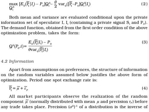 |
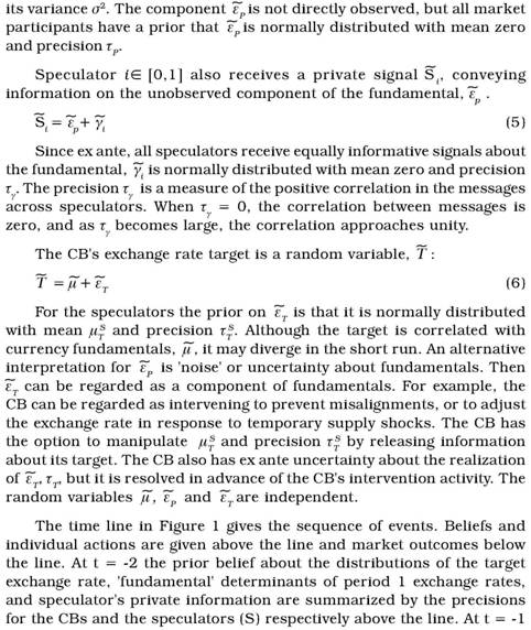 |
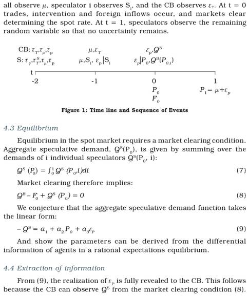 |
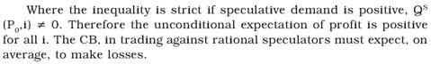 |
However, once the full heterogeneity of FX market participants are introduced in the model, rational speculators can make money from the less informed "noise" traders, and by providing insurance to hedgers. In order to prevent riskless "puts" against the CB, the band of variation of the managed float must not be less than ten percent, since then the risk of loss if the expected movement does not materialize becomes substantial. With a narrow band their loss is capped (Miller, 1997).
4.8 Managed Floating
In the case of a tightly managed float, more relevant to an emerging market such as India, where fundamentals are highly uncertain in a phase of rapid change, we can consider the unobserved component of the fundamental to be zero, since the spot rate is determined by fundamentals as revealed by CBs past targets and the CB's current targeting. This is an extreme case, to which an emerging market is likely to be closer. Speculators receive a private signal about the target, and expected future spot rate equals the expected target.
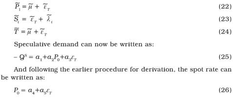 |
The perverse case does not exist. Intervention does not reveal the fundamentals as a2>0. Since there is no revelation of information from a signal, there is no conflict with the CB's target. So it is always worth the CB's while to signal.
Revealing some information about the target will allow the CB to achieve its targets partly through speculator trade, with minimal intervention (and therefore loss) and change in the interest rate (and therefore freedom to target the cycle). Such short-term exchange rate target changes in response to temporary supply shocks can reduce inflation, while minimizing decision lags. The homeopathic volatility induced deepens markets and reduce risk by encouraging hedging (Goyal, 2008).
Since political sensitivity to high inflation in a low per capita income country makes the CB unwilling to create inflation surprises and smoothing the impact of highly volatile inflows makes it willing to incur losses, Vitale's (2003) arguments about designing credible signals that make profits from reserve accumulation are not valid for an emerging market. Signals about the expected long run real exchange rate are helpful for exporters, and giving such signals is compatible with short-run nominal rate surprises to prevent the build up of speculative one-way positions. Since exporters would then hedge their short-term positions these fluctuations would not affect them. Thus Krugman's (1991) explicit target band is not required, but a signal of a nominal change will help converge markets to it, and like in his analysis, reduce the necessity for active CB action.
5. Conclusion and Policy Implications
We find evidence in both OLS and GMM regressions, and with monthly, daily and hourly data sets, that intervention affects the level of the exchange rate and its volatility. It has tended to depreciate the exchange rate, in the period of estimation, and reduce its volatility. A broader measure of intervention, derived from the RBI balance sheet, affects levels, while the RBI's reported measure affects volatility. Our results are robust also because the estimations use multiple data sets and variable definitions, carefully correct for simultaneity, for properties of the data, and include both policy and market variables.
Since intervention affects both the level of the exchange rate and its volatility, an independent exchange rate policy is feasible. Merchant net demand or order flow affects the level; dealer order flow and turnover variables affect the volatility of exchange rates. Intervention, merchant turnover and order flow increase dealer turnover. So microstructure variables are important. Net demand tends to be more important for levels and turnover for volatility. Merchant turnover is a driving force, perhaps because of the large inflows in the period as noted also in the survey of markets. Volatility and expected volatility increase dealer turnover. So policy should limit volatility in a diffuse ten percent band, but occasional surprise would serve as homeopathic medicine. Anticipated intervention decreases turnover, suggesting it is optimal to reveal information about future intervention. The coefficient of intervention on levels implies the estimated speculative demand curve is downward sloping in the spot rate. So expectations of future exchange rates and intervention are stabilizing and not perverse. A diffuse target contributes to market stability. The model of strategic interaction between the CB and speculators suggests that, to the extent there is greater uncertainty about fundamentals, speculative demand is always well behaved and the CB can optimally reveal more information.
Macroeconomic fundamentals represented by interest rate differentials have weak effects on exchange rate levels and volatility but strong effects on FX market turnover. So policy should reduce arbitrage gaps in interest rates. Estimated strategic market behaviour and model derivations both indicate intervention and signaling may be a more effective influence on exchange rates in the Indian context than interest rate changes. The latter should be targeted to the domestic cycle.
Markets form expectations of intervention activity and respond strategically to it. The increase in dealer turnover with intervention may imply strategic intraday arbitrage, whereby dealers profit at the expense of merchants and the CB. More transparency, whereby merchants are also aware of CB activity and targets may reduce the scope for such arbitrage. The disadvantage is that it may amplify the tendency for market agents to think alike, leading to large swings in variables. But since FX markets are predominantly bilateral and over the counter, agents will always have a range of information.
Signals about exchange rate changes, linked to random supply shocks, can generate surprise or enhance news, even while communicating clearly with the market. The markets will then help to bring them about, reducing the need for CB action. Transparency will reduce speculative positions and two-way movement of the nominal exchange rates will encourage hedging. Guidance to restrain nominal volatility within a ten percent band around a competitive exchange rate, but without committing to specific band edges, will maintain export competitiveness, helping the real sector.
References
Bhattacharya, U. and P. Weller. 1997. The Advantage of Hiding One’s Hand: Speculation and Central Bank Intervention in the Foreign Exchange Market. Journal of Monetary Economics 39: 251-77.
BIS (Bank of International Settlements). 2007. Foreign Exchange and Derivatives Market Activity in 2007. Triennial Central Bank Survey. December (accessed on 10/11/08). http://www.bis.org/publ/rpfxf07t.htm.
Blinder, A. S., Ehrmann, M., Fratzscher, M., Haan, J. D., and Jansen, D.-J. (2008). Central Bank Communication and Monetary Policy: A Survey of Theory and Evidence. Journal of Economic Literature, 46(4), 910-945.
Clarida, R., Gali, J., and Gertler, M. 1999. The Science of Monetary Policy: A New Keynesian Perspective. Journal of Economic Literature. 37 (4): 1661-707.
Dominguez, K.M. 2003. The Market Microstructure of Central Bank Intervention. Journal of International Economics. 59: 25-45
Dominguez, K.M., and J.A. Frankel. 1993. Does Foreign Exchange Intervention Work? Institute for International Economics: Washington D.C.
Edison, H. R. Guimaraes-Filho, C. Kramer, and J. Miniane. 2007. Sterilized Intervention in Emerging Asia: Is It Effective?. Regional Economic Outlook Asia and Pacific. October. International Monetary Fund: Washington
Geithner, T.J. 2004. Hedge Funds and their Implications for the Financial System. Federal Reserve Bank of New York.
http://www.newyorkfed.org/newsevents/speeches/2004/gei041117.html
Goyal, A. 2008. Incentives from Exchange Rate Regimes in an Institutional Context. Journal of Quantitative Economics, January&July, 6:1&2, 101-121.
Holub, T. 2004 Foreign Exchange Interventions Under Inflation Targeting: The Czech Experience. CNB Internal Research and Policy Note. Czech National Bank: Prague
Hüfner, Felix. 2004. Foreign Exchange Intervention as a Monetary Policy Instrument: Evidence for Inflation Targeting Countries. ZEW Economic Studies. Vol. 23. Springer.
IMF. 2008. India: Selected Issues. January. International Monetary Fund: Washington Krugman, P.R. 1991. Target Zones and Exchange Rate Dynamics. The Quarterly Journal of Economics. CVI, 3: 669-682.
Lyons, R. 2001. The Microstructure Approach to Exchange Rates. MIT Press: CA
Miller, M. 1997. Risk and Return on Futures Contracts: A Chicago View. Chapter 10: 92-100 in Merton Miller on Derivatives. John Wiley & Sons, Inc: New York
Onatski, A. and J. H. Stock. 2002. Robust Monetary Policy Under Model Uncertainty in a Small Model of the U.S. Economy. Macroeconomic Dynamics. 1 (February). 6: 85-110.
Pattanaik, Sitikantha and Sahoo, Satyananda. 2003. The Effectiveness of Intervention in India: An Empirical Assessment. RBI Occasional papers. June. Vol. 22
Rudebusch, Glenn. 2002. Assessing Nominal Income Rules for Monetary Policy with Model and Data Uncertainty. Economic Journal. April. 112: 402-432.
Sager, M.J. and Mark P. Taylor. 2006. Under the Microscope: The Structure of the Foreign Exchange Market. International Journal of Finance and Economics. 11: 81-95.
Svensson, L.E.O. 2000. Open-Economy Inflation Targeting. Journal of International Economics. 50: 155-183.
Svensson, L.E.O. and N. Williams. 2005. Monetary Policy with Model Uncertainty: Distribution Forecast Targeting. NBER W P. 11733.
Tarapore, S.S. 2006. Report of the Committee on Fuller Capital Account Convertibility. Reserve Bank of India: Mumbai
Vitale, P. 2003. Foreign Exchange intervention: How to Signal Policy Objectives and Stabilize the Economy. Journal of Monetary Economics. 50: 841-870.
Weiland, V. 2003. Monetary Policy and Uncertainty about the Natural Unemployment Rate. CEPR Discussion Paper. 3811.
Woodford, M. 2003. Interest and prices: Foundations of a Theory of Monetary Policy. Princeton University Press: NJ
Appendix
Charts 1: Monthly autocorrelation functions
Charts 1: Monthly autocorrelation functions (contd...)
Charts 1: Monthly autocorrelation functions (contd...)
Charts 1: Monthly autocorrelation functions (concld...)
Charts 2: Daily autocorrelation functions
Charts 2: Daily autocorrelation functions (contd.)
Charts 2: Daily autocorrelation functions (concld.)
Charts 3: Monthly data graphs
Charts 3: Monthly data graphs (contd.)
Charts 3: Monthly data graphs (contd.)
Charts 3: Monthly data graphs (concld.)
Charts 4: Daily data graphs
Charts 4: Daily data graphs (contd.)
Charts 4: Daily data graphs (contd.)
Charts 4: Daily data graphs (concld.)
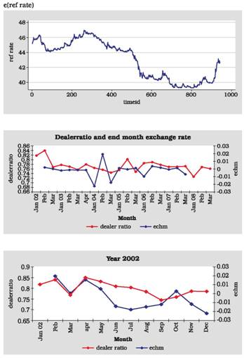 |
* Dr. Ashima Goyal is a Professor at Indira Gandhi Institute of Developement Research. Shri. R. Ayyappan Nair is Assistant General Manager, Financial Markets Department and Dr. Amaresh Samantaraya is Assistant Advisor, Department of Banking Supervision, RBI.
1 There are a number of papers in this field. Some key references are Weiland (2003) and Svensson and
Williams (2005). If robust preferences are assumed, the objective becomes to prevent the worst-case scenario,
and can imply a large monetary policy response. Onatski and Stock (2002) examine robust preferences.
Goyal (2009) shows shocks that reduce natural rates and therefore require a reduction in policy rates dominate
in a small open emerging market economy with a dualistic labour market.
2 Even countries following inflation targeting such as the Czech Republic, reconcile it with managed floats
by ensuring interest rates remain the primary tool of monetary policy, and any intervention works in the
same direction as interest rate changes (Holub, 2004).
3 The RBI view is that since exchange volatility is rising more hedging tools are required, and volatility must
be restricted until agents learn to manage. The point made here is that ensuring some volatility will improve
incentives to hedge.
4 Equations of the type common in the FX market microstructure literature (Lyons 2001, Dominguez and
Frankel 1993, Dominguez 2003), giving the response of the spot exchange rate to signed order flow, intervention,
and other relevant variables, are estimated.
5 Intervention data are only available ex-post, at the monthly frequency. Past research with this data has found that intervention does not affect the level of the rupee, but it reduces volatility (Pattanaik and Sahoo, 2003, Edison, 2007). Although the studies control for endogeneity using two-stage least squares techniques, our use of GMM and instruments for expected variables is more robust. These studies have also not used market microstructure variables.
6 The sources for much of the information in this section, unless explicitly mentioned, are various RBI publications and internal memos consulted by Ayyapan Nair and Amaresh Samantaraya.
7 Repos are financial instruments for the temporary exchange of cash against securities with a transfer of ownership.
8 This section is based on material in Lyons (2001), Sarno and Taylor (2002), Sagar and Taylor (2007), largely the latter.
9 This is only a proxy since daily liquidity management is not solely concerned with exchange rate
management, but also takes into account mismatches arising from government borrowing requirements,
fluctuation of government balances with RBI having implications for market liquidity and overall monetary
management. In addition, at the time of steep inflows during 2006-07 MSS was actively used for sterilization.
10 The standard narrow definition of intervention is CB purchases and sales of foreign exchange against
domestic currency. Dominguez and Frankel (1993) define it more broadly as any official transaction or
announcement intended to influence the exchange rate or stock of foreign exchange reserves. Hüfner (2004)
argues that change in reserves may be a more comprehensive measure of intervention than officially released
data on intervention, because measurement depends on what the CB sees as intervention, but all transactions
are reflected in the balance sheet. Passive intervention is said to be customer initiated but is actually a
misnomer, since the CB can always select the timing. The RBI’s intervention data reflects purchase and
sale of the US dollar including purchase/sale leg of swaps and outright forwards.
11 The interest differential is taken as given at zero, so that the spot rate would equal the forward rate |
 IST,
IST,