Press Release

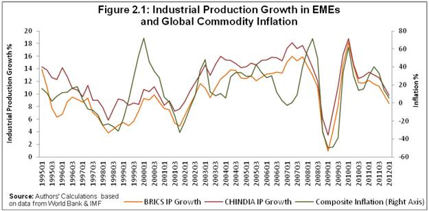
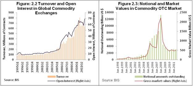
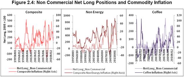
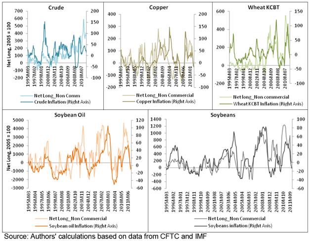
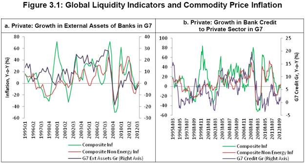
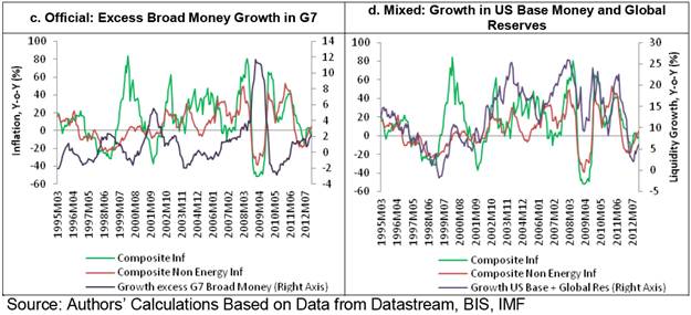
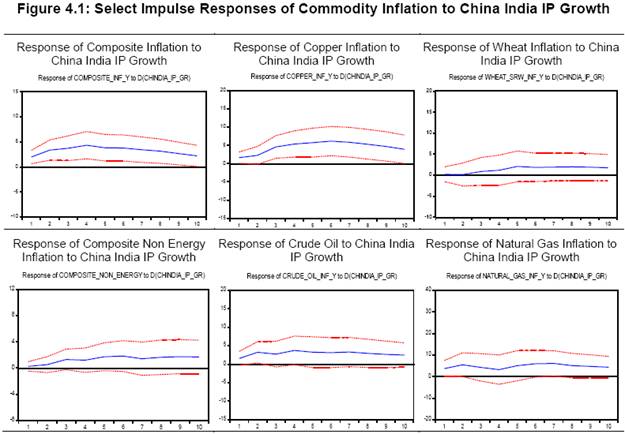
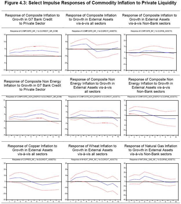
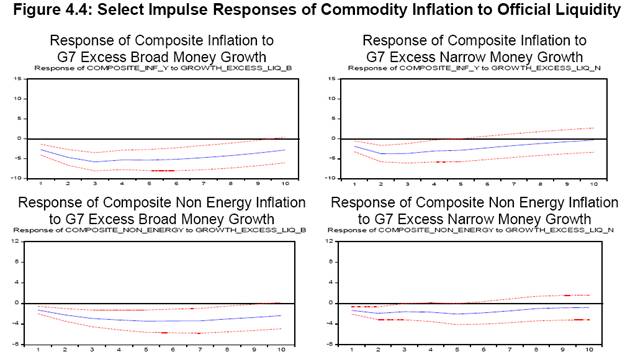
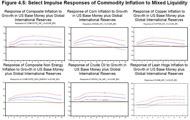
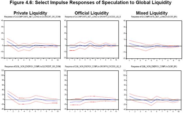
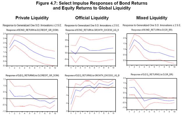
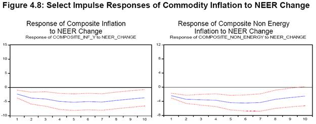
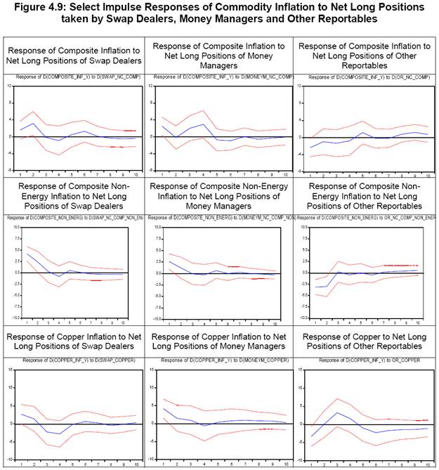
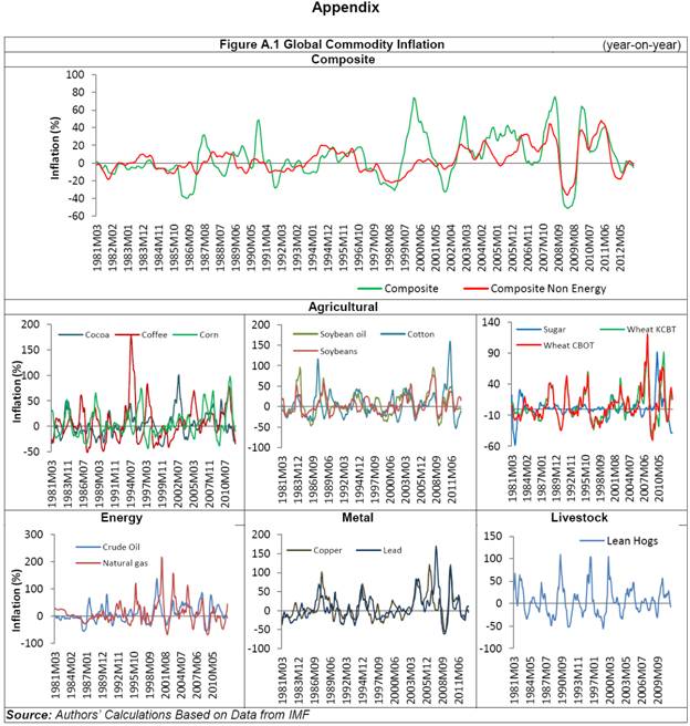
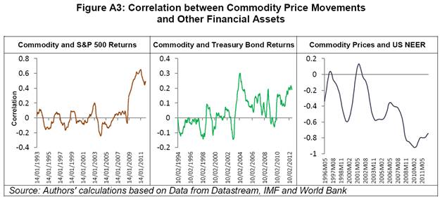
RBI Working Paper Series No. 01
Global Liquidity, Financialisation
and Commodity Price Inflation
^@Kumar Rishabh and Somnath Sharma

Abstract

¹ We review the role of the factors, identified in the literature, behind the global commodity inflation, viz. emerging market demand, speculation led by financialisation and easy global liquidity. This paper contributes to the existing literature on the issue in two ways. First, following BIS (2011), the distinction between ‘private liquidity’ and ‘official liquidity’ is applied to understand the indicators of inflationary pressures in the commodity market. Second, the impact of the activities of different type of non-commercial commodity derivative traders on commodity prices is studied. We find financialisation of commodity markets and emerging market demand have driven commodity price inflation. Further, ‘private liquidity’ is found to be inflationary while ‘official liquidity’ is not; possibly due to the central banks leaning against the wind since the financial crisis of 2008. We find that active traders like money managers along with the traditional passive swap dealers have played important role in commodity inflation dynamics.

Key Words: Commodity Prices, Inflation, Speculation, Global Liquidity, Emerging market demand, Official Liquidity, Private Liquidity, Index Investors, Swap Dealers, Money Managers

JEL Classification: E31, E50, E51, E52, G15, F30, F40, F53, Q10, Q40

Global Liquidity, Financialisation and Commodity Price Inflation

The excessive global commodity price volatility which started in the early years of the past decade continues to persist, posing significant policy challenges. Developments in the commodity prices in the recent years have been exceptional in several ways. According to UNCTAD (2011a), the episode of spectacular price increase between 2002 and mid 2008 and the collapse in prices following it, were most pronounced in several decades in terms of magnitude, duration and breadth as well as in terms of the number of commodities affected. Global commodity prices started to recover strongly since mid-2009, especially from mid-2010 onwards, reaching almost the pre-crisis level peak towards the mid of 2011. Since then, even though prices have shown two way movement, they still remain much elevated to the comfort of policy makers with the upside risk being substantial. More remarkably, the spectacular rise in commodity prices over the past decade has been accompanied by significant deviations of prices from their long term trend levels causing unprecedented price instability. The high instability has had significant negative macroeconomic consequences for the developing economies in terms of inflationary pressures and even real income losses. Recognising these challenges, G-20 leaders committed to ‘address excessive commodity price volatility’ as early as in the Pittsburgh summit in September 2009 (G-20 2009).

Researchers have identified several factors that may have contributed to high global commodity inflation (for example, Irwin, Sanders and Merin, 2010; Masters and White 2008; Gilbert, 2010). The fundamental factors, that have been suggested to have driven the recent commodity prices, include surging demand from rapidly growing emerging market economies like China and India and a relatively slow supply response and use of food grains for bio-fuel production etc. Commodity markets have also moved closely with the traditional financial asset markets like equity, bonds and the US dollar. This phenomenon of highly correlated movement between the financial markets and commodities has been prominent since almost the same time as the beginning of the commodity price boom and purported to have been driven by the movement of financial investors into commodities following deregulation of commodity and financial markets across the globe in the nineties and early 2000s. Increase in global liquidity since the beginning of the previous decade following easy monetary policy in most of the advanced economies is also considered as a reason for increased commodity prices (G20 (2011)).

In this paper we review the arguments put forth in the literature regarding the role of these factors, followed by an empirical analysis to ascertain the impact of the factors identified. Our paper contributes to the existing literature in following ways. First, a greater emphasis is laid on understanding the concept of global liquidity, facilitated mainly by, BIS (2011) and Domanski et al. (2011). Particularly, the distinction between ‘private liquidity’ and ‘official liquidity’ as defined in BIS (2011) is applied to examine if the two have a different / divergent impact on inflation and what can serve as a better indicator of inflationary pressures in the commodity market. Second, we also examine the dynamics of the various categories of the non-commercial commodity traders’ and their impact on commodity prices using the disaggregated commitments of traders (COT) data which the US Commodity Futures Trading Commission started releasing in September 4, 2006. The analysis on the new disaggregated data contributes to our understanding of the relative importance of different traders such that those who take passive positions (swap dealers) as against the money managers who trade actively.

The results of our empirical analysis suggest that financialisation of commodity markets and fundamental factors have played important roles since the early 2000s in driving commodity inflation. Growth in China’s and India’s demand is found to be positively associated with higher commodity inflation. Similarly, higher net long positions of non-commercial commodity traders are positively associated with inflation. The role of global liquidity in commodity prices is complex; the ‘official liquidity’ – characterized by global measures of monetary aggregates – is not found to be inflationary possibly due to the actions of central banks in leaning against the wind especially since the GFC of 2008. However, ‘private liquidity’ – based on the global credit aggregates – on the other hand is found to be inflationary in the period under study. We find the evidence that the private liquidity growth is positively associated with higher non-commercial traders’ net long positions which in turn are associated with higher commodity inflation suggesting global liquidity flows into commodity derivatives, leads to an increase in speculation resulting into higher commodity prices. Further, our results show that active traders like money managers along with the traditional passive swap dealers have played an important role in commodity inflation in the period under study.

The paper is organised as follows. In the first section we briefly analyse the trends in commodity prices over the last few decades. In the second section we review the arguments that have been extended to explain the exceptional rise in commodity prices since the early 2000s. Third section discusses the concept of global liquidity, issues concerning the measurement of global liquidity and its link with the commodity price speculation and prices. Fourth section presents the discussion on the data and methodology employed in our study and the results of the empirical exercise to determine the impact of the above mentioned factors on commodity inflation, using alternative measures of official, private liquidity and mixed liquidity and different sets of data on non-commercial net long positions. The final section concludes and discusses a few policy implications of the results.

1. Trends in Commodity Price Movements

High commodity price inflation and instability, since nearly the beginning of the 21st century have affected a wide range of commodities – from energy to agricultural commodities to metals. Prior to that commodity inflation remained subdued during 1980s and 1990s, in the so called period of ‘great moderation’. Figure A.1 gives the Year-on-Year (Y-o-Y) inflation for 13 highly traded commodities and for two composite categories viz. Non - energy and all 12 commodities. The composite series are constructed using IMF’s trade weights used for calculations of their own price indices. Average composite inflation for the 12 commodities during the 1980s was in fact negative and only marginally positive in the 1990s but increased to around 19 percent per annum during the period 2000-07 and was at 37 percent at its peak in 2008. The dramatic dip in prices in the next year was of the order of around 26 percent. The non-energy inflation which stood at its peak at 17 percent in 2008 and low at negative 14.5 percent in 2009 was much lower than the corresponding figures for the overall price inflation implying that this trend was largely driven by energy commodities. For example, the crude oil inflation in 2008 was 43 percent. Commodity prices recovered strongly in 2010 and 2011 with double digit inflation recorded in almost all the commodities. Since 2012 commodity prices have declined slightly however the risk of rebound persists.

Another feature of the commodity markets in the recent period has been extremely large volatility. High inflation and volatility have proved to be especially deleterious for the emerging and developing countries and their food security. Average global food prices at their peak in June 2008 were 270 percent higher than in 2002 and even after steeply falling in 2009 remained at 106 per cent higher than in 2002. Further, much in line with the other prices, food prices increased 87 percent between February 2009 and February 2011.

IMF (2011) contend that food price shocks have larger effects on headline inflation in emerging and developing economies than in advanced economies as pass-through tends to be larger for the former. “The median long-term pass-through of a 1 percent food price shock to domestic food prices is 0.18 percent in advanced economies and 0.34 percent in emerging and developing economies” (Ibid). In the case of India, Rajmal and Misra (2009) find that there is a less than complete pass-through from international to domestic food prices and it varies according to the import dependency. Dissecting the pass through of global food prices on Indian food prices, Chandrasekhar and Ghosh (2011) find that transmission is robust during the upward trend in the prices while some kind of ratchet effect exists in domestic prices during the downward trend in the global commodity prices. Moreover, it should be noted that even if the pass through coefficients are small, the price impact of pass through on domestic prices may still be high if large movements in the global commodity prices, say of the tune as discussed above, take place.

2. Drivers of Commodity Inflation

There is a lively debate on what factors are responsible for the commodity price rise. On one side are those who argue that the rise in commodity price is driven by the fundamental factors of demand and supply (for example Irwin, Sanders and Merin, 2010) while the others argue that the financialisation of commodity markets have had a larger role (for example, Masters and White 2008, Gilbert, 2010). Another empirical study (Tang and Xiong, 2010) that included both fundamental and financial variables concluded that growing demand from emerging economies was not the only driver of the commodity price hike in 2006–2008 but also financialisation which remained significant even after controlling for fundamental factors. Similarly, Kaufmann et al. (2008), who have attempted to explain oil price developments on the basis of supply and demand levels, refinery capacity and expectations, contend that since the second half of 2007 the actual prices rose more rapidly and started to exceed the already increasing predicted prices (based on fundamental factors) by a substantial margin, indicating that that fundamental supply and demand factors pushed prices upwards starting from 2003, but in 2007–2008 prices rose above their fundamental levels. Tang and Xiong (op.cit) tried to capture the growing role of index investment in the commodity price formation by looking at the co-movement between the prices of different commodities after 2003–2004, and they found that for the commodities included in the major indexes the increase in co-movement was significantly more pronounced than for those not included. We look at these factors in detail in the following sections. The report of the G20 Study Group on Commodities (April 2011) provides a comprehensive review of the literature in this regard.

2.1 Fundamental Factors

The first fundamental factor that has been identified is the demand from emerging market economies (EMEs) – especially India and China. The argument, in short, is that since the EMEs are at a relatively commodity-intensive stage (see Table 1 in Appendix) of development and as these countries have grown faster, the industrial demand for metals and energy and consumption demand for higher protein foods such as livestock and dairy has soared. Indeed the co-movement between commodity inflation and emerging market growth is quite significant especially since early 2000s (Figure 2.1).

On the supply side, factors that might have had an impact on the inflation include the diversion of both land and certain agricultural output (i.e. corn, sugar, oilseeds and palm oil ) for bio-fuel production, rising costs of inputs, falling land productivity etc. According to IMF (2008), bio-fuel production has expanded in response to rising fuel prices, as well as due to government subsidies, and tariff protection in major advanced economies. World bio-fuel production, which was 0.3 million barrels per day in 2000, increased at a trend growth of 19 percent per annum for ten years to 1.9 million barrels per day in 2010. The phenomenal growth in bio-fuel production has particularly changed the usage structure of corn. For example, in the US, around 2 per cent corn produced every year was used for fuel in the 1980s (5 percent in 1990s) but now more than 35 percent of corn supplies every year go for producing fuel which is 46 percent of the corn used domestically in the country (4 percent in 1980s, 7 percent in 1990s). This indicates the scale to which acreage and output of corn must have been transferred over time for bio-fuel production.

But are these factors enough to explain the trend in price movements and inflation? A closer look would suggest maybe not. For example, if the demand and supply factors were the sole source of the rise in prices and instability up to the mid 2008 the subsequent fall in prices and instability in relatively very short periods of time may not be tenable. Also, the FAO data suggest that the demand-supply mismatch may not have been enough to have generated such high instability in the prices in such a short duration of time. FAO data show that the world stock to use ratio for cereals, although had declined modestly until 2007-08 compared from that of earlier years but since then had consistently increased and remained at healthy levels of above 20 with global supply growth outstripping growth in utilization. This overall trend may justify an increase in price up to 2007-08 but by such a huge magnitude, is untenable. More so, another round of increase of prices and instability since the second quarter of 2009 in the environment of increasing stock to use ratio casts doubt over the argument that only fundamental factors were responsible for the movements in price and instability. Most of the other factors which are often cited as drivers of commodity price, such as population growth or changing consumption patterns have been at work for a long period and have often even coincided with low commodity prices and therefore their role in explaining recent sharp price hikes is doubtful (UNCTAD 2011b).

2.2 Financial Factors

Financialisation of commodity markets refers to an increased involvement of financial investors in the global commodity derivative markets. The financialisation of the commodity markets coincides with the broader financialisation trends witnessed in the era of financial liberalization across the world, especially in advanced economies (UNCTAD 2011a).

Financialisation is said to have led to excessive speculation in the commodities market. Traditionally, commodities futures markets had two categories of participants: Physical Hedgers and Speculators. Physical Hedgers participate in the commodity futures market to reduce or eliminate the price risk they face from their commercial activities in the spot markets and their decisions to trade or hedge is strictly based on supply and demand fundamentals. Speculators, on the other hand, do not have any underlying physical commodity position to hedge but they trade to profit from changes in futures prices. Speculators have an essential function in the commodity futures market of providing liquidity by accepting price risk and in a market dominated by the buying and selling decisions of physical hedgers, the speculators will also base their trading decisions on those same supply and demand fundamentals (Masters and White 2008).

However, what has become controversial is the role of a new kind of investors – the Index investors. According to Masters and White (2008), “Index Speculators are Institutional Investors engaged in commodities futures trading strategies that seek to replicate one of the major commodities indices by mechanically following that index’s methodology.” According to U.S. CFTC, “the investors engaging in index activity in commodity markets include index funds, swap dealers, pension funds, hedge funds and mutual funds. They also include exchange traded funds (ETFs), exchange traded notes (ETNs) and similar exchange-traded products that have a fiduciary or other obligation to track the value of a commodity or a basket of commodities in an essentially passive manner.” The institutional investors engage in index investment activity primarily through two ways – direct investment in futures markets and indirect investment through over-the-counter (OTC) swap agreements with financial firms. While direct investment involves investment by the money managers on behalf of the institutional investors in the commodity futures exchange, in an index swap investors get exposure to the commodity markets through swap dealers who pay a return based on the value of a specified index to the investors. Basically, an OTC swap dealer offers the investors a return on a commodity index, for example S&P GSCI and DJUBSI, against a known fixed return, say on a treasury bill, along with some fees. After selling a swap contract, the swap dealer hedges its own exposure to the swap contract by purchasing the corresponding futures contracts in the commodity index. (Tang and Xiong, 2010)

The emergence of index investors in the early 2000s has been associated with a rapid rise in the global commodity futures market activity, in terms of turnover and open interest (Figure 2.2).

The OTC market activity also grew rapidly from the year 2004, in line with the organised exchanges, but fell sharply at the end of 2008 and in 2009 (Figure 2.3), as the commodity index traders started to unwind their positions owing to significant larger counterparty risks (Jörg Mayer, 2009).

The OTC market since then has remained relatively subdued, perhaps reflecting the concern of the investors that OTC markets are to be tightly regulated after the financial crisis of 2007-08. This trend also indicates that the direct active investment in commodity exchanges has become more prominent as against passive swap arrangements, as the role of money managers may have increased post crisis.

The emergence of Index investors followed two broad developments viz. the deregulation of commodity markets and the emergence of commodities as an asset class like equity, bonds and currency. Commodity markets in the US were regulated since the 1936 when the Commodity Exchange Act had placed limits on the size of speculators positions, to ensure the dominance of bona fide Physical Hedgers. However, in 1991 exemptions from position limits to swap dealers for the purposes of hedging their OTC swaps transactions were started to be given as it was believed that the swap dealers were also only hedging to offset the exposure they have in the OTC market (Masters and White, 2008). Further in 2000, the Commodity Futures Modernization Act (CFMA) deregulated commodity trading in the United States, by exempting over-the-counter (OTC) commodity trading from CFTC oversight (Ghosh 2011). In the following years, the notional amount outstanding in the commodity OTC markets rose from around US$ 60 billion in December 1999 to more than US$ 13 Trillion in June 2008. Commodities became attractive for hedging as they carried premium for idiosyncratic commodity price risk as over the business cycle commodity price return is negatively correlated with that of other asset classes (Gorton and Rouwenhorst, 2006), in contrast to traditional assets like equities and bonds which carry premium only for systematic risk and are highly correlated with market indices and with each other (Tang and Xiong, 2010). Figure A1 in the appendix shows the correlation between S&P 500 equity index returns and S&P GSCI commodity Index returns as well as the correlation between the JP Morgan Treasury index returns and with the latter. The correlations were negative or zero until the initial years of 2000s, after which they became significantly positive especially around and after 2008-09 indicating that the financial and commodity markets have moved pretty closely since then indicating a high degree of financialisation.

Commodity prices also move opposite to the movement of the US dollar and therefore Investing in commodity futures contracts may provide a hedge against changes in the exchange rate of the dollar (Figure Appendix A3). The negative co-movement works majorly through two channels. First is through the purchasing power and cost channel – as most commodities are priced in U.S. dollars. Dollar depreciation makes commodities less expensive for consumers in non-dollar regions, thereby increasing their demand. The other is the asset channel – a depreciating U.S. dollar reduces the returns on dollar-denominated financial assets in foreign currencies, and thus makes commodities more attractive class of alternative assets to foreign investors. Also, dollar depreciation raises risks of inflationary pressure in the United States, prompting investors to move toward real assets – such as commodities – to hedge against inflation. The dollar appreciation, on the other hand will have a dampening effect on commodity prices. (IMF 2008)

Recognition of potential diversification benefits from investing in the commodities futures markets drove the rapid growth of commodity index investment since early 2000 leading to financialisation of the commodity markets. The reason for increased inflow of investment in commodities in the early 2000s, (after it was allowed following the deregulation as discussed above) was because other financial markets crashed during the dotcom bubble burst at the end of 2001. Another jump in the index investment occurred in 2008 as the subprime mortgage crisis in the US deepened and spread, when speculators started investing in food and metals.

To summarise, according to the financialisation argument, the high commodity prices since the early 2000s up to the latter half of 2008 was due to index investors pouring in money in the commodity futures markets. The subsequent decline in prices occurred as the investors started unwinding their positions in commodities, when the losses in the US housing and other markets became huge and it became necessary for many funds to book their profits to cover losses or provide liquidity for other activities.

Figure 2.4 presents evidence on co-movement between net long positions (Long positions minus short positions) of non-commercial traders, as defined by CFTC, and the commodity spot prices. Noncommercial traders in the CFTC’s data reflect only money manager portion of the index investors but leave out swap dealers due to the “swap dealer loophole” where the CFTC classified swap dealers as commercial traders².

3. Global Liquidity and Commodity Prices

An issue related with the financialisation of the commodity market is that it has become exposed to the risk of price bubbles, like other asset classes, following excess global liquidity flows. In a financialised market, easy global liquidity conditions can affect commodity prices through changes in investment dynamics that are independent of fundamentals, as the lower return on safe assets may shift financial investments into riskier assets. In this context it becomes imperative to identify the relevant indicators of global liquidity that may be important for tracking the build-up of asset prices. However, it is very difficult to define global liquidity as the term is used in a variety of ways and in different contexts, making it a challenging task to accurately quantify.

Given the elusive nature of the concept of global liquidity, authors have used different measures to proxy for global liquidity in order to assess its impact on inflation in general or on commodity and other asset prices. Mostly, these measures center on the monetary aggregates and their variants. For example, Agostino and Surico (2009) define global liquidity as the mean or the first dynamic principal component of the growth rates of broad money across the G7 economies. Sousa and Zaghini (2007) construct a measure of global liquidity as the sum of the reference monetary aggregates for the US, the Euro area, Japan, the UK and Canada by converting each national aggregate into Euros using PPP exchange rates.

As far as the studies concerning global liquidity and commodity prices are concerned, Belke et. al. (2009), using broad monetary aggregate in major OECD countries as a measure of global liquidity, concluded that global liquidity could be considered as a useful indicator of commodity price inflation. Chakraborty and Bordoloi (2012) use the concept of excess liquidity, defining it as the deviation of the money supply from its trend estimate. They found significant impact of excess liquidity on commodity prices although their results also suggest a lesser impact of liquidity on the commodity prices in the more recent time period.

Bank for International Settlements’ (BIS) Committee on the Global Financial System (CGFS) made an attempt to delve into the issues on the measurement, drivers and policy implications of global liquidity. Its report (BIS 2011) serves as one of the most comprehensive treatment of the issue and forms a considerable part of our discussion here. In the context of global liquidity, BIS emphasizes the need to distinguish between private and public liquidity for the two have different dynamics although they interact in obvious ways. Domanski et al. (2011), explain private liquidity as the liquidity that “...is created by private sector market participants, including international banks, institutional investors, and non-bank financial institutions (including shadow banks) and so on.” Further, “Movements in private liquidity are transmitted internationally through the cross-border and/or cross-currency operations of bank and a non-bank financial institution......Private liquidity is endogenous to the conditions in the global financial system. It depends on the willingness of market participants to supply funding or trade in securities markets.”

In contrast to private liquidity, official liquidity is funding provided by the public sector. Official liquidity is the funding that central banks provide and is considered to be exogenous. Central banks create official liquidity in their domestic currency through regular monetary operations and, during periods of stress, through emergency liquidity assistance. From this perspective, the most obvious indicators of official liquidity are narrow and broad money aggregates. However, the private and official liquidity concepts are not totally independent and interact in various ways. (Domanski et al. 2011)

On the use of indicators of global liquidity, BIS contends that broad global credit aggregates, ideally comprising bank- and non-bank credit, provide an indication of liquidity creation by the private sector and can help track global private liquidity cycles. The most important reason for using such credit aggregates is that “private sector credit stands at the end of the financial intermediation chain and captures the interaction of market and funding liquidity…. Moreover, credit aggregates have been shown to behave as early warning indicators, especially when combined with measures such as asset prices.” (Domanski et al. 2011)

Lane (2012) provides an insight how low cost financing and commodity markets are linked through the process of financialisation of commodity markets. According to Lane (2012);

“A central element in the financing of commodities leading up to the 2008 crisis was the increasing participation of major global investment banks. Because of their access to wholesale funding markets, which provided them with cheaper funding than was available to other participants in commodity markets; the large banks became increasingly important in a range of commodity - related activities. They provided a large share of the lending to commodity dealers. They also themselves came to play a central role as dealers in over - the - counter derivatives markets in commodities. More recently, they have become more and more involved in the physical trading of commodities: holding physical inventories, making markets in commodities and even creating supply chains by providing shipping and commodity storage.”

We present the evidence on the co-movement of global liquidity and commodity prices in Figure 3.1.

4. Data, Methodology and Results

4.1 Data

Commodity Prices

We calculate commodity year-on-year (y-o-y) inflation for 12 commodities viz. cocoa, coffee, copper, corn, cotton, crude oil (NYMEX), lean hogs, natural gas, soybean, soybean oil, sugar and wheat from different categories – agricultural, energy, metal and livestock. The data on global commodity price indices (with 2005 as base year) are available with monthly frequency for more than 50 commodities in the IMF primary commodity database. We construct a composite price index by taking the weighted average of the 12 chosen commodity indices. The weights used for estimating the composite price index of 12 commodities³ are calculated by transforming the weights of the commodities which IMF uses for its all commodity price index. The weights⁴ employed by the IMF are based on 2002-2004 average world export earnings. The 12 commodities included in our study together carry more than 70 percent weight in the IMF all commodities index. We have taken only 12 commodities into consideration because the corresponding continuous time series data on the commodity derivatives are available for this set of commodities. We further separate the energy commodities (crude oil and natural gas) from the chosen 12 commodities and construct composite non-energy price index after adjusting for the weights. We separate the energy commodities so as to control for bias that may be caused due to high weights of these commodities in the composite index.

Speculation

In order to capture speculation, we have looked into the positions taken by the non-commercial traders. To capture the activities of non-commercial traders we take the US CFTC weekly reports on the commitment of traders (COT). The US commodity derivatives market, according to the BIS, constitutes around 40 percent of the total global commodity derivatives market size in terms of volume of trade. Another advantage of using the US CFTC data on the COT is that it is available participant-wise allowing us to identify positions taken by non-commercial traders.

The data on the COT is available in two formats - old format which has data separately on two broad categories of trader’s viz. commercial and non-commercial traders; and the new format that further disaggregates these categories. In the old format “commercial” trader category includes producers, merchants, processors and users of the physical commodity who manage their business risks by hedging. It also includes swap dealers that may have incurred a risk in the over-the-counter (OTC) market and then offset that risk in the futures markets, regardless of whether their OTC counterparty was a commercial trader or a speculator. In the new format, therefore, the swap dealers have been taken separately. The new format also includes money managers and other reportables that correspond to the ‘non-commercial’ category in the old format. Money managers are the traders who are engaged in managing and conducting organized futures trading on behalf of their clients. Traders those are not placed into swap dealers and money managers are placed into the other reportables category. Hence, the new disaggregated format increases transparency from the old format by separating traders into further categories. However, there is a trade-off in using the old and the formats of data i.e. the data on the old format is available from March 1995 while, the disaggregated COT is available only from June 2006. For our purpose we have taken commodity-wise data on commitments of non-commercial traders in the old aggregated format as well as the COT of non-commercial traders in the new disaggregated format separately.

We calculate the commodity-wise net-long position of the non-commercial traders by taking the difference of ‘long all’ position and ‘short all’ position of the non-commercial traders. We then transform the net-long positions of the non-commercial traders into indices by taking the average net-long positions during the year 2005 equal to 100. We also estimate the composite net-long positions of the commodities based on the weighing scheme adopted by us in the calculation of the primary commodity price index. Here again we calculate the composite net-long position of the non-commercial traders and further separate the non-energy commodities and calculate non-energy composite net-long positions using the same methodology as adopted in the calculation of the composite price index and composite non-energy price index respectively. For the disaggregated data also we separately calculate the commodity-wise net-long positions taken by swap dealers, money managers and other reportable as well as their respective composite net long positions and composite non-energy net-long positions.

Global Liquidity

We have used different indicators of global liquidity which can be broadly classified as – private liquidity, official liquidity and one that can be called a mix of the two. All these indicators have been used in the literature in similar or different contexts and explanation on each are in order. For private liquidity we take the total external asset positions of the G7 banks in all currencies vis-à-vis all sectors and vis-à-vis non-bank sectors as suggested by BIS (2011) which are available with a quarterly frequency in BIS locational banking statistics. Movements in private liquidity are transmitted internationally through the cross-border and/or cross-currency operations of global banks. We take into account only the G7 banks into consideration as the data on these countries is available continuously and these countries together account for about 61 percent of the total external asset positions of the international banks vis-à-vis all sectors and about 67 percent of bank assets vis-à-vis non-bank sector.

Since the measure on cross border bank assets is available only with a quarterly frequency we use another measure of private global liquidity so as to obtain data on monthly frequency. This indicator is the GDP weighted growth in bank credit to the private sector in the G7 countries. This indicator is a proxy for private global liquidity to the extent that domestic liquidity conditions in the advanced economies can spill over to global markets (BIS 2011). Data on G7 bank credit to the private sector is collected from Datastream and data on GDP is from IMF World Economic Outlook (WEO) database. Annual GDP weight for a country is derived using GDP measured in U.S. dollars at market exchange rates as a share of G7 GDP. This is in accordance with the IMF methodology of using the nominal GDP at market exchange rate for aggregating monetary indicators. Annual GDP weights are applied to all 12 months of a particular year for a country to calculate the weighted average.

Our official liquidity indicators are obtained based on the methodology employed by Baks and Cramer (1999). First we create weighted average series of monthly money supply for the G7 countries, in which the growth rate of money for each G-7 country (in domestic currency terms) is weighted by the respective country's GDP share when taken in U.S. dollars. Weights are again annual, applied to all 12 months. In the second step, the weighted average GDP growth is obtained for the G7 at a quarterly frequency where the growth rate of nominal GDP (in local currency) for each G7 country is weighed by the country’s GDP (calculated in US dollar) share in the G7. As a final step we find excess money growth by subtracting the average GDP growth from the average money supply growth series. Average GDP growth for a particular quarter is used for all the three months comprising it when subtracting from the average money supply growth. Same method is applied to both narrow and broad money to find ‘excess narrow money growth’ and ‘excess broad money growth’ respectively. Monthly money supply series are from Datastream while quarterly GDP series are from the OECD.

The final indicator of global liquidity is constructed following Darius and Radde (2010) where they have used US base plus global international reserves as a measure to capture the availability of a global medium of exchange. This indicator can be considered as a mixed indicator of private and official liquidity as defined by us above. According to BIS (2011), literature points to a positive interaction between official and private global liquidity through the reinvestment of foreign exchange reserves. BIS contends that, the reinvestment of the forex reserves in issuing countries’ liquid assets contributes to easing financial conditions, causing additional capital outflows and reserve accumulation to the host countries. This feedback loop acts as an amplification mechanism on the original monetary impulse and its impact on global liquidity.

Emerging Market Demand

In absence of the monthly data on GDP we take industrial production as a proxy for demand. The Industrial production data are from the Global Economic Monitor database of the World Bank. We calculate a combined industrial production as the sum of industrial production (constant US $ with the same base) and calculate the growth rate viz. Chindia IP growth.

Exchange Rate

To analyse the change in the price of commodities due to change in the US dollar exchange rate we use Nominal Effective Exchange Rate (NEER) of US dollar from the Global Economic Monitor database of the World Bank. NEER is a measure of the value of a currency against a weighted average of several foreign currencies. An increase in the value of NEER means the appreciation of the US dollar vis-à-vis the basket of other currencies.

Other Asset Classes

Investment in commodity derivatives also helps financial investors in diversification of risks; hence, if the derivatives markets are generally doing well, we may see a positive correlation among all the financial asset classes. We take daily S&P 500 composite price index from Datastream and calculate y-o-y equity price returns⁵ at the daily frequency and then average it to convert it to monthly equity price return series and quarterly equity price return series. To calculate the bond price returns we take the Citigroup ‘All Maturity World Government daily Bond Index’ from Datastream which is a market capitalization weighted bond index consisting of the government bond markets of the multiple countries. Analogous to our estimation of equity price returns, we calculate monthly and quarterly bond price returns series.

Appendix Table A2 gives the information on all the variables used in the analysis and their source.

4.2 Empirical Analysis and Results

We first adjust all the variables for seasonality using the Census X12, Additive method. We then test for the stationarity of the series. As the different data series we use for our analysis are of different order of integration (Appendix Table A3), we are not able to do any test for long-run relationship inter alia cointegration analysis. In whichever case the data series is found to be I(1), we take the first difference of that series. We fit in an unrestricted Vector Auto Regression (VAR) model to find the main drivers of commodity inflation because this approach allows us to fully capture the interaction among macroeconomic variables and their feedback effects. By avoiding the need for structural modeling, unrestricted VARs allow for the identification and analysis of mechanisms by which economic time series interact without making any a priori assumptions regarding the exogeneity or endogeneity of the concerned variables. By treating each variable endogenously, VARs consider each series as influenced by the lagged values of all the endogenous variables in the system, including its own, which allows for general patterns of interaction to emerge, and thus facilitates the analysis of potential transmission mechanisms.

An unrestricted VAR with a lag length p is defined as:

where, Yt is a kX1 random vector, the Ai are k X k fixed coefficient matrices, V is a kX1 fixed vector of intercept terms, and Ut is a k X1 white noise process. The error terms satisfy the white noise condition if their expected mean value is zero, there is no autocorrelation, variance is constant, and are normally distributed.

The purpose of our analysis here is to investigate the impact of different factors viz. demand factors, speculation, global liquidity and exchange rate on the commodity inflation. To do that we fit in simple VARs with separate measures of global liquidity, speculation, inflation, EME demand and other variables (NEER Change, Equity Return and Bond Return) as endogenous variables. We do this analysis for all the 12 commodities taken into consideration here and the commodity groups viz. composite commodities and composite non energy commodities.

We present here as an example one of the several VARs we run for our analysis. For instance if we want to check the impact of private liquidity along with identified fundamental factors, speculation and other factors on the composite commodity inflation in the period 1995M03 to 2012M12, we set up a VAR on – first difference of China and India IP Growth (d(chindia_ip_gr)), first difference growth in G7 bank credit to private sector (d(credit_gr_dom)), bond return (bond_return), first difference of equity returns (d(eq_returns)), change in nominal exchange rate (neer_change), first difference of composite net long (d(composite_net_long)) and composite inflation (composite_inf_y) as the endogenous variables. We set the lag length equal to 4 which is consistent with the results of the test for optimal lag length. VAR (4) is the correct specification here as the residual series are found to be multivariate normal and are not serially correlated. The specified model also meets the stability condition, which requires that no roots lie outside the unit circle.

We then analyse the impulse responses and variance decompositions obtained from these VARs and explain the impact of different factors - demand factors, speculation, global liquidity and exchange rate - on the commodity inflation. Since the parameters of unrestricted VAR models are difficult to interpret, impulse response functions and variance decompositions are generated to understand the dynamic relationships between the variables. Impulse response functions delineate the effect of a one-time shock to one of the variables on current and future values of the endogenous variables thus indicating the directions of their dynamic relationships. We have used the generalised impulse response functions with one standard deviation shock to endogenous variables. Generalised impulse response functions generate the impulse responses without any ordering. Variance decompositions show the relative importance of each variable in determining the values of all the endogenous variables in the system over different time periods, by separating the proportion of the movements in a series that is due to innovations in its own values compared with the other variables.

Following the steps explained in the example above, we fit unrestricted VARs for the 12 commodities and two commodity groups separately. In other words, we run VARs for each commodity (or commodity group) with different combinations of global liquidity indicators and a set of other variables explained in the example above. We explain here impact of each factor in the commodity inflation. For the sake of brevity only relevant and important results are presented.

Emerging Market Demand

The impact of a one-time positive shock in the Chindia IP growth is associated with a significant increase in composite commodity inflation. The increase in commodity inflation also displays considerable persistence over time; however, the impact of a one-time positive shock in the Chindia IP growth on composite non-energy inflation is insignificant. On doing a commodity wise analysis this impact of a one-time positive shock in Chindia IP growth is found to vary across commodities as is observed from the impulse responses obtained from different VARs (Figure 4.1).

Among the Non-energy commodities, the impact of Chindia IP growth on – wheat, coffee and corn inflation is found to be insignificant while on copper inflation it is found to be positive. On the other hand, the impact of Chindia IP growth on energy commodities viz. Crude oil and natural gas inflation are found to be positive. This can be explained by the fact that China and India are primarily the large importers of metals and energy commodities due to the rising demand as a result of high growth rates. This does provide evidence towards the widely believed notion that the rise in global commodity prices may be due to high demand arising from China and India particularly for metals and energy, however, this may not explain the rise in most of the non-energy commodities inflation.

Speculation

Speculation in the commodities derivatives market which is measured by the net long positions of the non-commercial traders also play a big role in commodity inflation. The impulse responses obtained from the VARs (Figure 4.2) show that composite net long position (composite_net_long) has a positive impact on the composite inflation (composite_inf_y). Moreover, the impact of composite non-energy net long position (nl_non_energy_comp) on the non-energy commodities group inflation (composite_non_energy) is found to be persistent as observed from the variance decomposition (Table 4.1).

Commodity wise analyses show that the speculation as measured by the net long positions taken by the non-commercial traders has a significant positive impact on the inflation of all the commodities taken into consideration in our analysis, except natural gas. The supply of natural gas, in the past decade, has increased from the unconventional sources (like shale gas). So, the impact of speculation is not observed in the natural gas as the increasing supply may have slowed down the rise in natural gas prices (IMF 2011). Overall, we find that speculation does have a positive impact on the commodities inflation.

Global Liquidity

A. Private liquidity

We find that a one-time positive shock on the growth in bank credit to the private sector of the G7 countries (credit_gr_dom) has a significant positive impact on the commodity inflation. Its impact is found to be positive both on composite commodity inflation as well as composite non-energy inflation as is observed from the impulse responses obtained from the VARs (Figure 4.3) with credit_gr_dom as a measure of private liquidity. To test the robustness of our results, we obtain the impulse responses from the VARs with growth in G7 banks external assets vis-à-vis all sectors (grext_assets) and vis-à-vis non-bank sector (grnb_assets) as well (Figure 4.3). These credit aggregates are closer to the characterization of global private liquidity that is mainly channeled through international banks. As explained earlier, data on these aggregates are available in quarterly frequency, so the VARs are fit on the quarterly average of the monthly variables. We find that a positive shock in the grext_assets and grnb_assets have a significant positive impact on composite commodity inflation, however, their impact varies across commodities. We do not find impact of a one-time shock in grext_assets on composite non-energy inflation; however, it is not the same across all the non-energy commodities. For example, it has a positive impact on copper and wheat inflation. Similarly, the impact of grnb_assets on commodity inflation is not same across all the commodity groups – no significant impact on composite commodities inflation but a significant impact on non-energy composite inflation. Overall, we find the evidence of the positive impact of private liquidity on commodity inflation.

B. Official Liquidity

The impact of a one-time positive shock in the official liquidity on commodity inflation, however, is found to be negative. The impulse responses obtained from the VARs using G7 excess broad money growth (growth_excess_liq_b) and G7 excess narrow money growth (growth_excess_liq_n) (Figure 4.4) as measures of official liquidity, show that positive innovations in these variables have a negative impact on the commodity inflation all across the commodities and commodity groups taken into consideration. The negative impact of official liquidity on commodity prices may be because of the central banks ‘leaning against the wind’ i.e. expanding liquidity while growth in the global economy was ailing and commodity prices decreased. In such periods, we would, thus, expect negative rather than positive relationship between official liquidity and commodity prices.

C. Mixed Liquidity

The impulse responses (Figure 4.5) obtained from VARs with US Base Money plus global International Reserves (gr_br) as a measure of liquidity shows that it has a positive impact on the commodity inflation. The positive impact of mixed liquidity on commodity inflation is found across all the commodities and commodity groups – composite commodities and composite non-energy commodities.

D. Global Liquidity and Speculation

In order to understand the channel of flow of liquidity to commodity markets, we analyze the impact of global liquidity on commodity speculation from the impulse responses obtained from the VARs with different measures of global liquidity. We find that there is a positive impact of private liquidity and mixed liquidity on speculation, however, the impact of official liquidity on speculation is not found to be significant. The negative impact of official liquidity on commodity inflation is also mirrored on the insignificant impact of official liquidity on commodities speculation for the reasons discussed earlier.

As far as the other asset classes are concerned, on analysis of the impulse responses (Figure 4.7) we find that the private liquidity and mixed liquidity both have a positive impact on the bond and equity returns while the impact of official liquidity on bond returns is insignificant and its impact on equity returns is negative. This result also explains the co-movement and high positive correlation between the commodity and equity prices and commodity and bond prices.

Changes in Exchange Rate

We analyse the impact of variations in the dollar exchange rate on commodity prices by looking into the impulse responses (Figure 4.8) obtained from the VARs. We find that one time positive shock in US NEER i.e. dollar depreciation has a negative impact on commodity prices across all the commodities and commodity groups taken into consideration here. This indicates both valuation effect and the asset side effect discussed earlier.

An Analysis with the Disaggregated Data on Traders Positions

As explained earlier, CFTC now releases disaggregated data on COT in which the positions taken by the non commercial traders have been disaggregated to positions taken by swap dealers, money managers and other reportables. This data is available monthly since 2006 and it separates the positions taken by swap dealers which were earlier clubbed with the positions taken by the commercial traders. In this analysis we fit in different sets of VARs with disaggregated net long positions by the non commercial traders viz. swap dealers, money managers and other reportable with different measures of global liquidity in a similar procedure described above. We then analyse the impulse responses obtained from these VARs. We find that a one-time shock in the net long positions taken by the swap dealers and money managers have a significant positive impact on commodity inflation across all the commodities and commodity groups taken into consideration (Figure 4.9). However, the impacts of net long positions taken by other reportables are found to be insignificant in case of composite commodity inflation and negative in case of composite non-energy inflation. We also present here the variance decomposition obtained from one of the VARs with G7 bank credit growth as a measure of private liquidity (Table 4.2). We find that among the non commercial traders, net long positions of Money Managers (MONEYM_NC_COMP) and Swap Dealers (SWAP_NC_COMP) have major impact on composite price inflation. It shows that the activities of money managers and swap dealers in the commodity derivatives market are the major drivers of commodity inflation. In fact among a few commodities, money managers seem to be playing more important role than the swap dealers. For example, in case of copper, we observe through impulse responses, that a one-time shock in the net long positions of the swap dealers and money managers in copper has a significant positive impact on the copper inflation. Analysing the variance decomposition (Table 4.3) of copper inflation, we find that relative importance of net long positions taken by money managers in copper in determining copper inflation is high as compared with net long positions of swap dealers and other reportable.

5. Conclusion

We find that both financialisation of commodity markets as well as fundamental factors have driven global commodities price inflation. The role of global liquidity in commodity prices is found to be complex; the ‘official liquidity’ – characterized by measures of global monetary aggregates – is not found to be inflationary while the private liquidity growth is found to be associated with higher commodity inflation.

Our analyses using US CFTC COT data on the non-commercial trader net long positions both in the old format where swap dealers are excluded from the category – due to the so called ‘swap dealer loophole’ – and in the new format where we have net long positions available separately for swap dealers and other non-commercial traders viz. money managers and other reportable show that speculation plays an important role in determining commodity inflation. We find the impact of speculation to be positive on commodity inflation for our composite groups as well as for most of the commodities indicating that speculation in commodity markets remains an important factor explaining high commodity inflation. This result has a significant implication as it is recognised that in a financialised market where speculation thrives, the price of a commodity is no longer just determined by fundamental factors but may also be driven by the risk appetite for financial assets and investment behaviour of financial investors and this is damaging as far as the traditional roles of futures markets is concerned. In a financialised commodity market, risk of speculative bubbles and prolonged deviations of prices from those justified by fundamental factors may distort economic activities and make hedging costly for commercial users owing to the greater uncertainty caused by financial investors (UNCTAD 2011a).

Recognising the deleterious impact that high commodity prices can have for the food security and of the unbridled speculation on the market functioning and price volatility, the G-20 leaders in 2009 at the Pittsburgh summit and in the subsequent summits requested the International Organization of Securities Commissions (IOSCO) to develop and implement OTC derivatives market reforms and specifically called for all standardised OTC derivatives to be traded on exchanges or electronic platforms, cleared by central counterparties (CCPs) and reported to trade repositories. The IOSCO (2011) in its report ‘Principles for the Regulation and Supervision of Commodity Derivatives Markets’ in September 2011, inter alia, recommended granting of authority to financial regulators to impose position limits on commodity derivatives as a means to prevent market manipulation. The G20 (2011) endorsed these principles at its summit in Cannes in November 2011. As far as the implementation of the reforms is concerned, on the OTC front, on May 16, 2013, the U.S. CFTC adopted several rules relating to swap execution. New U.S. rules requiring many OTC derivatives to be traded on swap execution facilities (SEF) make the U.S. the first country to implement the G20 economies’ commitments on derivatives made after the crisis. However, CFTC has not been able to put position limits on the derivatives traders. CFTC’s earlier attempt to introduce limits on the size of positions that market participants could take in futures and over-the-counter swaps linked to 28 physically delivered commodities were thwarted in late September 2012 by a US court orders following fierce opposition by traders and many energy market participants.

There are two important issues as far as the regulation of the global commodity derivatives markets is concerned. First is that, while financial regulation in the US may be important, it may not be enough as a large share of trading also takes place at other centres including in the European, Japanese and Singaporean exchanges while some new centres are also emerging. In the absence of legislations globally, the speculative activity will simply move to other financial centres. Further, the problems of cross-border difference in rules may again provide opportunities for speculators to exploit those and then there are cross border cooperation issues. Also, there are data gaps that may hinder the cross-border surveillance. For instance, trader category wise data is available only in the US and Europe lags significantly behind in that compared to US exchanges.

Secondly, so far the need for tighter regulation has been discussed mainly as the need to reform the OTC market segment. However, as the OTC markets are increasingly regulated, financial investors are likely to move away from investing passively in indexes towards a more active trading behaviour blurring the difference between short-term oriented managed funds and swap dealers. This underlines the importance our second set of results based on the disaggregated level analysis done across different type of non-commercial traders. Our results clearly point out how money managers have played an important role across commodities. Indeed, for most of the commodities, the impulse responses and variance decomposition suggested a bigger role for money managers than swap dealers. In fact, the recent fall in OTC activity points to a decline in the relative importance of the use of swaps and an increasing relative importance of more sophisticated active trading in futures contracts traded on commodity exchanges. A survey conducted by Barclays (2012) concluded that the broad-based index investing was now the least favoured option among investors with much greater interest in external asset manager and dynamic index approaches.

As a novel approach to understanding commodity market dynamics in the context of global liquidity, we look beyond the monetary measures conventionally used in the literature. We differentiate between official and private liquidity. The results provide interesting insights into the interaction between global liquidity and commodity inflation. As far as the broad categories of global liquidity indicators employed by us are concerned, we find an opposite impact of private and official liquidity. While private liquidity shocks are found to be inflationary almost across all commodities, official liquidity, defined as excess liquidity, is associated with a declining inflation. This result could very well be driven by the fact that the central banks across the world were more concerned about growth in a significant portion of the period under study and were leaning against the wind. A mix of both the measures, as proxied by the sum of US base money and global reserves, is also found to be associated with higher inflation across most of the commodities. There are a few considerations, however, in this regard that are important. Official and private global liquidity are not independent and interact in several ways – for instance private sector perceptions of the availability of official liquidity may affect risk taking. However, as asserted by the BIS (2011) an element of private liquidity is endogenous as the key determinant of the funding conditions in the modern financial system is the behaviour of the financial sector, and its willingness to provide cross- border and/or foreign currency financing. Financial innovation facilitates creation of instruments that enhance market or funding liquidity by allowing new means of payment BIS (2011). This feature of global private liquidity is appreciated in the context of its role in explaining commodity inflation in the recent times where global monetary aggregates have found to have lost their explanatory power. Our results point that the private liquidity has to be watched more closely in conjugation with monetary aggregates by the policy makers for the buildup of inflationary tendencies in the commodity markets. In the broader context, since the private liquidity is considered to be endogenous, our results imply that direct regulation of speculation may be more effective in restricting speculation (and to that extent consequent inflation) than the monetary policy measures.

Finally, given growing emerging market demand plays a role in higher commodity inflation especially in the energy and metal commodities, policy responses should aim to address fundamental demand supply imbalances. These measures include easing supply constraints, removing restrictions on the supply or export of major commodities and investment in productive capacity.

^@ Kumar Rishabh (email) and Somnath Sharma (email) are Research Officers in the Department of Economic and Policy Research, Reserve Bank of India.

¹ Views expressed in the paper are those of authors and not of the Bank. The authors are grateful for useful comments from an anonymous referee.

² The CFTC began publishing a Disaggregated Commitments of Traders (Disaggregated COT) report on September 4, 2009. The Disaggregated COT report increases transparency from the legacy COT reports by separating traders into the following four categories: Producer/Merchant/Processor/User; Swap Dealers; Managed Money; and Other Reportables. The legacy COT report separates reportable traders only into “commercial” and “non-commercial” categories.

³ For calculating the weighted average of all the commodities we have divided the weight of wheat equally between the Soft Red Winter Wheat and Hard Red Winter Wheat.

⁴ Available at http://www.imf.org/external/np/res/commod/Table2.pdf

⁵ Returns_y-o-y = [(P_t,year- P_t,year-1)/ P_t,year-1]*100

References

Agostino A. and Surico P. (2009), “Does Global Liquidity Help to Forecast U.S. Inflation?”, Journal of Money, Credit and Banking, 41 (2 – 3), 479 –489.

Baks, Klaas and Kramer, Charles (1999), “Global Liquidity and Asset Prices: Measurement, Implications, and Spillovers”, IMF Working Paper, WP/99/168, 1999

Barclays (2012), “The Commodity Investor” February 29, 2012

Belke, A.; Bordon, I.G. and Hendricks, T.W. (2009), “Global Liquidity and Commodity Prices – A Cointegrated VAR Approach for OECD Countries”, DIW Berlin Discussion Papers, German Institute for Economic Research, No. 898.

BIS (2011), “Global liquidity - concept, measurement and policy implications”, CGFS Publications No 45 November 2011.

Chandrasekhar, C.P. and Ghosh, Jayati (2011), “Food Price Transmission in South Asia” The Hindu Business Line, June 14, 2011

Chakraborty, Asit B and Bordoloi, Sanjib (2012) “International commodity prices – volatility and global liquidity” Bank for International Settlement, Proceedings of the Sixth IFC Conference on "Statistical issues and activities in a changing environment" Basel, 28-29 August 2012, IFC Bulletin No 36 February 2013.

Darius, Reginald and Radde, Sören (2010), “Can Global Liquidity Forecast Asset Prices?”, IMF Working Paper, WP/10/196

Domanski, Dietrich, Fender, Ingo and McGuire, Patrick M (2011), “Assessing global liquidity”, BIS Quarterly Review, December 2011

FAO (2010), “Undernourishment around the world in 2010”, The State of Food Insecurity in the World 2010

G20 (2009), “G20 Leaders Statement: The Pittsburgh Summit”, September 24-25, 2009

G20 (2011), Communiqué, G20 Leaders Summit – Cannes – 3-4 November 2011

G20 (2011), “Report of the G20 Study Group on Commodities under the chairmanship of Mr. Hiroshi NAKASO”, November 2011

Ghosh, Jayati (2011), “Commodity Speculation and the Food Crisis” in Lilliston, Ben and Ranallo, Andrew (ed) Excessive Speculation in Agriculture Commodities: Selected Writings from 2008–2011, Institute for Agriculture and Trade Policy (IATP), April 2011

Gilbert, Christopher L. (2010) “How to Understand High Food Prices”, Journal of Agricultural Economics, Vol. 61, No. 2, 2010, 398–425, 2010

Gorton, G.B. and K.G. Rouwenhorst (2006), “Facts and fantasies about commodity futures”, Financial Analysts Journal 62, 47-68, 2006

IMF (2008), “World Economic Outlook”, April 2008

IMF (2011), “World Economic Outlook”, September 2011

Irwin, Scott H, Dwight R Sanders, and Robert P Merrin (2009), “Devil or Angel? The Role of Speculation in the Recent Commodity Price Boom (and Bust)”, Journal of Agricultural and Applied Economics 41(2): 393 – 402

International Organization of Securities Commissions, IOSCO (2011), “Principles for the Regulation and Supervision of Commodity Derivatives Markets” released September 2011.

Jörg Mayer, 2009. "The Growing Interdependence Between Financial And Commodity Markets," UNCTAD Discussion Papers 195, United Nations Conference on Trade and Development.

Kaufmann, Robert K., Stéphane Dées, Audrey Gasteuil and Michael Mann (2008) “Assessing the Factors behind Oil price changes”, ECB working paper series No. 855, January 2008

Lane, Timothy (2012), “Financing commodities markets”, Remarks at the CFA Society of Calgary, Calgary, Alberta, 25 September 2012

Masters, Michael W., and Adam K. White (2008), “The Accidental Hunt Brothers: How Institutional Investors are driving up Food and Energy Prices”, http://accidentalhuntbrothers.com/.

Rajmal and Misra, Sangita (2009), “Transmission from International Food Prices to Domestic Food Prices - The Indian Evidence” RBI Staff Studies No. 08, Reserve Bank of India (September 22, 2009)

Sousa , J.M. and Zaghini, A. (2007), “Global Monetary Policy Shocks in the G5: A SVAR Approach”, Journal of International Financial Market, Institution and Money, 17(5), 403 – 419.

Tang, Ke, and Wei Xiong (2010), “Index Investing and the Financialisation of Commodities”, Working Paper, Department of Economics, Princeton University

UNCTAD (2011a), “Post-crisis policy challenges in the world economy”, Trade and Development Report.

UNCTAD (2011b) “Price Formation in Financialised commodity markets: the role of information”

Wray, L. Randall (2010), “The Commodities Market Bubble: Money Manager Capitalism and the Financialisation of Commodities”, The Levy Economics Institute of Bard College Public Policy Brief No. 96, 2008 (Highlights, No. 96A)