Press Release

RBI Working Paper Series No. 11

Inflation Forecast Combinations – The Indian Experience

Joice John^*, Sanjay Singh and Muneesh Kapur^@

Abstract

¹ Accurate, reliable and unbiased forecasts of inflation are critical for the monetary policy decision making process, more so for a flexible inflation targeting central bank. Inflation forecasting is, however, turning challenging across countries. This paper explores the merits of forecast combination approaches for improving the inflation forecasts in the Indian context. The results seem encouraging. The inflation forecast combination approach based on the performance-based weighting scheme outperformed the individual models both for headline inflation as well as core inflation for the longer horizons relevant for monetary policy. Overall, while the performance-based inflation forecast combinations add value to the forecasting exercise, ongoing structural transformations, greater role of global factors and recurrent weather shocks continue to pose challenges to the forecasting process.

JEL Classification: C53, E37, E52

Keywords: Inflation Forecast, Forecasting Accuracy, Forecast Combinations, Monetary Policy, India

Introduction

Given these complexities of inflation dynamics, central banks often use a suite of models approach, supplemented with informed judgment, for improving the quality of the forecasts. Underlying this preference is a tacit recognition that all models are misspecified in some dimension and at some points of time. In this context, a forecast combination approach – combining forecasts from alternative models through a judicious weighting system – finds favour among practitioners.

After the seminal work of Bates and Granger (1969), forecast combinations are considered as an effective and simple way to enhance the forecasting performance of the individual models. Forecast combination often outperforms even the ‘best’ forecasting model and “combining multiple forecasts leads to increased forecast accuracy” (Clemen, 1989, p.559). The widely popular M-Competitions (Makridakis competitions), comparing 100,000 time series and 61 forecasting methods in M4, found that “…of the top-performing methods, in terms of both PFs (point forecasts) and PIs (predication intervals), were combinations of mostly statistical methods, with such combinations being more accurate numerically than either pure statistical or pure ML (Machine Learning) methods” (Makridakis, Spiliotis and Assimakopoulos, 2020, p.60-61). Coming more specifically to economic and financial time series, Stock and Watson (2004) found clear empirical advantage of combining the forecasts in terms of lower pseudo-forecast errors. Even though there is a plethora of empirical studies supporting the superiority of forecast combinations over individual forecasts, the exact statistical rationale for this is not clearly understood. Intuitively, forecast combination performs better than the individual forecast for the following three reasons (Bjornland et al., 2012). First, as different models generally use different information set, the forecast combination may outperform individual models a la the portfolio diversification approach. Second, in the presence of unknown instability (structural break), different models may perform better at different points in time. The forecast combination may be more robust in the presence of such time-varying instabilities. Finally, forecast combination can help in addressing unknown biases, especially idiosyncratic ones due to omitted variables. Available evidence suggests that the forecast combination approach can also improve upon the inflation forecasts of individual models (Bjornland et al., 2012; Hubrich and Skudelny, 2017; RBI, 2017) and such findings motivate the present paper.

India moved to a formal inflation targeting framework in 2016 and, therefore, inflation forecasts have assumed a greater role in the conduct and formulation of monetary policy. Inflation forecasts by the Reserve Bank of India (RBI) in terms of accuracy and bias are comparable to major central banks (Raj et al., 2019; RBI, 2020). However, a substantially large share of food in the CPI basket in India and high volatility in food prices due to frequent weather shocks add to the complexities of inflation forecasting and management in India. A number of papers have focussed on alternative approaches to inflation analysis and forecasting. For example, the Phillips curve approach to inflation assessment and forecasting has been undertaken in Kapur (2013), Patra, Khundrakpam and George (2014) and Behera, Wahi and Kapur (2018). The role of non-linearities in the inflation-output relationship has been examined in RBI (2019). Structural vector autoregression approach has been assessed, inter alia, in Mohanty and John (2015); threshold regressions were used in Nachane and Lakshmi (2002), Mohanty et al. (2011) and Pattanaik and Nadhanael (2013); and time-varying parameter regressions were employed in John (2015). In contrast to a large literature on assessing individual models and approaches, there are only a few studies on inflation forecast combination approach in the Indian context (RBI, 2017; Dholakia and Kadiyala, 2018).

Against this backdrop, this paper empirically examines the performance of forecast combination approach for inflation over individual models, the benchmark random walk model and the median/mean forecasts of inflation from the Survey of Professional Forecasters (SPF) conducted by the RBI. As regards the individual models, the paper considers 26 individual models and 3 different combination approaches for the period Q1:2001-02 to Q4:2018-19 for the comparative assessment. While headline inflation remains the target for monetary policy, core inflation often provides a better indicator of underlying inflation and the future inflation path (Mishkin, 2007). Hence, the forecast combination approach has been attempted for core inflation also. The paper’s empirical analysis shows that the performance-based weighting scheme outperforms the individual models both for headline inflation as well as core inflation. Even the simple average of the forecasts from different individual models turns out to be comparable with the forecast from the ‘best’ performing individual model i.e., the forecasts from the models which performed best at each horizon. The performance-based forecast combination outperforms the best individual model forecasts and the average forecast by quite a margin at the longer horizons which matter more for the monetary policy decisions. Thus, consistent with the available evidence for other countries, the forecast combination methodology improves upon the individual models in the Indian context. However, in presence of large unanticipated shocks to exogenous variables – such as monsoon deficiency, unseasonal rainfall, crude oil prices, and exchange rate – the actual inflation outcome can still deviate substantially from the combined forecasts.

The paper is organized into five sections. Section II presents a brief review of studies on the inflation forecast combination approach. The analytical framework, data and sources are presented in Section III. The results are discussed in Section IV, with concluding observations in Section V.

II. Literature Review

The forecast combination approach² has a very long history. Seminal work of Bates and Granger (1969) combined two separate sets of forecasts of airline passengers based on their forecasting performance and found improvement in the combined forecast in terms of a lower forecasting error. In Nelson (1972), the combination of individual forecasts of macroeconomic variables, with weights based on their forecasting performance by using regression technique, outperformed individual models. Aiolfi and Timmermann (2006) investigated the forecasting performance of a large set of linear and non-linear time series models for G7 countries. The empirical results pointed to strong persistence in the forecast performance of individual models and the forecast combination - using various schemes such as trimming, pooling shrinkage estimation and optimal weights - resulted in a better overall forecast for a set of macro-variables.

Moving specifically to forecast combination approaches in the context of inflation modelling, a number of central banks such as the Bank of England, Sveriges Riksbank, Reserve Bank of New Zealand and Bank of Canada make use of combination approaches to improve upon the individual model forecasts or to do a cross-check on the forecasts of their key models. For the UK, while the individual models did not often beat the forecasts from the benchmark autoregressive model, the combination forecasts frequently outperformed the benchmark (Kapetanios, Labhard and Price, 2008). For Norway, combination forecasts improved upon the point forecasts from individual models and interestingly the central bank’s (Norges Bank’s) own forecasts for inflation at all horizons, even as the latter had the benefit of expert judgement. The gains increased with the forecast horizon. Some degree of trimming of the model space – i.e., trimming to keep a small sub-group of the best performing models, varying across time – contributed to the combination forecasts outperforming the policymaker’s forecasts (Bjornland et al., 2012). For Turkey, forecast combination turned out to be better than most of the individual models, although only marginally. The performance of the Bayesian VAR models was close to the superior models at each horizon (Öğünç et al., 2013).

For the US, a comparison of combination forecasts suggests that the models using equal weights for combining forecasts did not produce worse forecasts than those with time-varying weights. Variable selection, time-varying lag length choice, and stochastic volatility specification are, however, important for the outperformance of combination forecasts (Zhang, 2019). For the euro area, the relative performance of the different models differs considerably over time. The superiority of forecast combinations was confirmed for core inflation, with performance-based weighting combinations outperforming simple averaging (Hubrich and Skudelny, 2017). For headline inflation, however, the superiority of combination forecasts was time-varying. Forecast combinations were also better than individual models in turning point predictions (i.e., the fraction of times forecasts predicted a change in the right direction) for core inflation; for headline inflation, however, the combination approaches underperformed some of the individual models.

While a number of studies, as noted above, find evidence in favour of performance-based combinations, some studies question this assessment. Hibon and Evgeniou (2005) examined performance of unweighted forecast combination for a large set of indicators and found no inherent advantage of forecast combinations over the best individual model; however, selecting the best individual model from a set of available models is difficult. In the context of output growth forecasts, Stock and Watson (2004) find that combination approaches often improve upon autoregressive forecasts; however, simple combinations such as mean/median turned out to be better than performance-based combination forecasts, a phenomenon they dub as ‘forecast combination puzzle’. On the whole, at least in the context of inflation dynamics, the subject matter of this paper, the available empirical evidence suggests that performance-based combinations have the scope of improving upon simple combinations.

For India, the combination forecasts were found to be more accurate than the eight individual models – random walk (RW), autoregressive (AR), moving average with stochastic volatility (MA-SV), vector autoregression (VAR), Bayesian VAR, VAR and BVAR with exogenous variables (VAR-X and BVAR-X, respectively) and Phillips curve (PC) (RBI, 2017). Similarly, Dholakia and Kadiyala (2018) considered RW, vector error correction, ARIMA, ARIMA-X, VAR and VAR-X models for the evaluation and found that no individual model outscored others at all horizons. Combination forecasts based on inverse mean squared error (MSE) were better than the combinations based on the simple average and median. However, the MSE weighted combination did not outperform the best individual model at all the horizons considered. Although the forecasting exercise was done in a pseudo-out-of-sample fashion, the study, however, used actual values for exogenous variables for the forecasting period.

Drawing upon the studies briefly reviewed in this section, we supplement the existing India specific studies in a number of ways - experimenting with a larger array of individual models, comparing different combination approaches, assessing the performance of forecast combinations by trimming the underperforming models, alternative time periods, and more forecast horizons. We also undertake the analysis not only for headline inflation but also for core inflation.

III. Empirical Framework

III.1 Inflation Forecasting Models

Given the objective of this paper is to examine the relative forecasting performance of combination-based approaches relative to individual models, the paper identifies a suite of econometric models that have been extensively used for predicting inflation drawing from the existing studies (Bjørnland et al., 2012; Dholakia and Kadiyala, 2018; Gilchrist and Zakrajsek, 2019; Hubrich and Skudelny, 2017; Öğünç et al., 2013; RBI, 2017). Phillips curve type models remain relevant if inflation expectations are weakly anchored and remain useful in times of large slack in case of well-anchored inflation expectations. Time-series models can be a better tool in case of a moderate slack in the economy and high credibility of the inflation target. Therefore, univariate and multivariate models on the one hand and time series and structural models on the other are used in the analysis, belonging to the following 12 category of models: (i) a random walk (RW) model; (ii) autoregressive (AR) models; (iii) moving average (MA) models; (iv) autoregressive moving average (ARMA) models; (v) AR models with conditional heteroscedasticity; (vi) MA models with conditional heteroscedasticity; (vii) ARMA models with conditional heteroscedasticity; (viii) Phillips curve models; (ix) vector autoregression (VAR) models; (x) VAR-X model, i.e., VAR models with exogenous variable/s; (xi) Bayesian VAR (BVAR) model; and (xii) BVAR-X, i.e., BVAR model with exogenous variable/s. As we try alternative lags in AR and MA models, and alternative variables/ specifications in Phillips curve and VAR/BVAR models, we obtained 26 models. The exact specifications/ representations of these models are given below:

i) Random Walk (RW) model: The random walk model is described as:

Where π_t is the annualized rate of quarter-on-quarter (q-o-q) percentage change in seasonally adjusted consumer price index (combined) (CPIC) inflation rate and ε_t is a random disturbance term which has expected value of zero.

ii) Autoregressive Model (AR): An autoregressive model of order p [AR(p)] assumes that the value of the target variable at time t depends on its values in the previous ‘p’ time periods plus a constant term.

iii) Moving Average (MA) Model: A moving average model of order q [MA(q)] assumes that the target variable is a linear combination of past error terms (ε) (upto the time period q) plus a constant term.

iv) Autoregressive Moving Average Model (ARMA): Combining AR(p) and MA(q) models results in an autoregressive moving average (ARMA) model of order (p,q) [ARMA(p,q)].

The order for AR(p), MA(q) and ARMA(p,q) models, explained above ((ii) to (iv)), were decided by following Akaike Information Criterion (AIC) and Schwarz Information Criterion (SIC).

v) - vii) Models with Generalized Autoregressive Conditional Heteroscedasticity: The models ii to iv above assume that the variance (σ²) of disturbance term is homoscedastic. To account for the breach of this assumption, the models ii to iv are augmented with a variance equation.

viii) Phillips Curve Models (PC): PC models relate inflation to the strength of economic activity in the economy, controlling for supply shocks such as swings in crude oil prices and exchange rates. Although the Phillips curve framework has faced significant criticisms in recent years given the disconnect between inflation and output across countries, the approach remains relevant once the various factors impinging upon the inflation dynamics are properly accounted for in the empirical analysis. For example, as Forbes (2019) has noted, domestic output demand-supply gap still matters for inflation dynamics, although with a diminished force due to globalisation; global factors - commodity prices, world slack, exchange rates, and global value chains – have now become significant drivers and their role in the inflation movements has increased over the last decade. External openness of the economy through exports and imports can potentially impact inflation dynamics through greater competition (Gilchrist and Zakrajsek, 2019). We use alternative indicators of economic activity like real GDP growth rate and the output gap. The collapse in the international crude oil prices (Brent) by over 60 per cent in just less than two months - from around US$ 60 a barrel in early February 2020 to below US$ 20 a barrel by April 2020 and a rebound to around US$ 40 by June 2020 – once again highlights the role of supply shocks in the inflation process and the need to incorporate them in the empirical framework. To capture these possible channels, we have used the following alternative PC specifications (6-10) for inflation forecasting: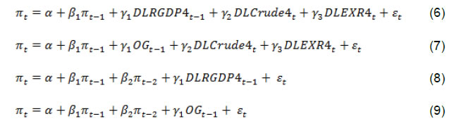

Where, DLRGDP4, DLcrude4 and DLEXR4 are annualized rate of q-o-q percentage change in seasonally adjusted real GDP, crude oil price, and exchange rate (INR/USD), respectively. OG is output gap³. TrGDP is an indicator of external openness, measured as the ratio of non-oil merchandise trade (i.e. exports plus imports) to nominal GDP.

ix) Vector Autoregression (VAR): The vector autoregression (VAR) model used for forecasting a system of interrelated time series variables can be represented as:

Where, y_t is a vector of k endogenous variables and p is the order of VAR (i.e. VAR(p)).

x) Vector Autoregression with exogenous variables (VARX): The vector autoregression (VAR) model regressed with a vector of exogenous variables can be represented as:

Where, y_t is a vector of k endogenous variables and p is the order of VAR (i.e. VAR(p)). F_t is a vector of d exogenous variables.

xi) Bayesian Vector Autoregression (BVAR): Combining all the right-hand side variable of a VAR(p) expressed above into a vector xt with the dimension of (kp) and corresponding coefficients into B as:

The VAR considers the coefficient vector B to be unknown but fixed and which can be estimated. On the contrary, the Bayesian Vector Autoregression (BVAR) approach assumes B vector as variables with some known distribution (a prior distribution). The parameters of the prior distribution are known as hyperparameters. For this study, the prior distribution of B vector has been taken as a multivariate normal distribution with known mean B* and covariance matrix V_b. This prior is known as Minnesota prior or Litterman’s prior (Litterman, 1979 and 1980).

xii) Bayesian Vector Auto regression with exogenous variables (BVARX): The Bayesian Vector Auto regression model is augmented with a d-dimensional exogenous vector (F_t).

As in the case of BVAR, the prior distribution of B vector has been taken as a multivariate normal distribution with known mean B* and covariance matrix V_b.

In VAR and BVAR models, we include real GDP growth rate (or output gap), inflation rate and policy rate as endogenous variables. Apart from these endogenous variables, the various models include exogenous variables like crude oil price (Indian basket) in United States Dollar (USD) terms, exchange rate (Rupees per USD, INR-USD), and trade to GDP ratio (TrGDP). While real GDP growth and output-gap (OG) are endogenous variables in VAR/BVAR, these are treated as exogenous variables in Phillips curve specifications. For generating the pseudo out-of-sample inflation forecasts for evaluating the model performance, the exogenous variables were projected by using an AR(1) model rather than using their actual values. The significant recurrent volatility in some of these variables – international crude oil price and exchange rate – highlights the forecasting complexities.

III.2 Inflation Combination Methods

The forecasts of individual models are combined by using the following three alternate approaches following Hubrich and Skudelny (2017).

i) Simple (unweighted) average of the forecasts from all the models.

ii) Inverse RMSE: Performance-based weighted average of inflation forecast, with weights being inverse of mean squared (pseudo out of sample) forecast error (MSFE) of respective models, calculated for a rolling window of preceding 8 quarters’ forecasts relative to the sum of MSFE of all the models: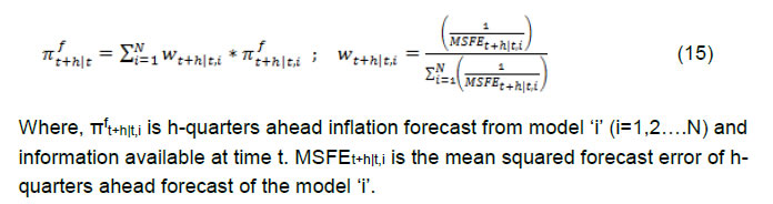

iii) Geometric Decay: Performance-based weighted average inflation forecast combination with geometrically decaying weights combines the performance of individual models with time dimension of performance. Relative to the previous (inverse-weighting) approach, this weighting scheme gives more weight to the recent performance relative to earlier performance, and this is done through an exponential function. Accordingly, the inflation forecast combination for geometric decay weighting scheme is done in two steps:

Step I: h-quarter ahead geometric decay weighted MSFE error of the last 8 quarters (i.e. the rolling window of 8 quarters) for the model i is calculated as:

Where, constant λ is a decay factor⁴.

Step II: Then, the inflation forecast combination is done as: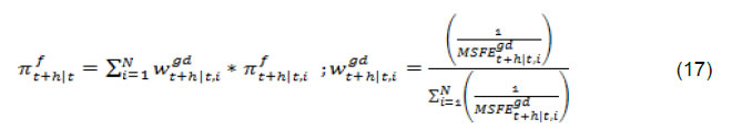

As noted earlier, the paper explores 26 individual models, three combination methods, two different rolling windows (viz., 24 and 32 quarters) and two different inflation metrics (headline inflation and core inflation). As a result, 4,988 inflation forecasts series were generated for the full sample period (Q1:2001-02 to Q4: 2018-19) and another 1,740 forecasts were generated for the shorter sample period (Q1:2011-12 to Q4:2018-19). These were augmented by 1,392 forecasts from auxiliary models for exogenous variables. Altogether, this study generated forecasts from 8,120 models using Matlab routines⁵.

III.3 Data

The headline inflation measure is based on the consumer price index (combined) (CPIC). Core inflation is often calculated by removing the volatile components/ sub-groups in the consumers’ consumption basket. Although there is no official measure of core inflation, CPI excluding food and fuel in the Indian context is often treated as a suitable measure of core inflation (Raj et al., 2020). Hence, CPIC inflation excluding food, fuel and light is taken as the measure of core inflation. The National Statistical Office (NSO) started compiling CPIC in 2011; RBI (2014) provided back-casted data on CPIC for 2001-2010, using data on CPI-Industrial Workers (CPI-IW)⁶. Therefore, the period of study was taken from Q1:2001-02 to Q4: 2018-19 and data frequency was chosen as quarterly⁷. As the CPIC prior to 2011 in RBI (2014) was back-casted largely based on the retail prices faced by industrial workers, the paper also undertakes, as a robustness exercise, analysis for the smaller sample period (Q1:2011-12 to Q4:2018-19) for which the actual data on CPIC are available.

A brief review of the inflation dynamics since the early 2000s indicates that inflation was rather moderate during 2001-2007; it rose to double-digit levels in 2010 and saw a substantial disinflation from 2014 (Chart 1). The headline inflation declined to 2.5 per cent in Q4:2018-19 from 11.1 per cent in Q4:2010-11. Beginning 2007, CPI inflation rose mainly due to higher global commodity prices, especially those of crude oil. A deficit monsoon led to a further rise in food inflation in 2009 and its persistence contributed to elevated inflation expectations and generalised inflation. The double-digit inflation led to a review of the extant multiple indicators framework of monetary policy and a phased switch to a flexible inflation targeting framework in 2014 (RBI, 2014). In 2016, the flexible inflation targeting was formally adopted following amendments to the Reserve Bank of India Act, 1934. A monetary policy committee was constituted, with the objective of achieving the medium-term target for consumer price index (CPI) inflation of 4 per cent within a band of +/- 2 per cent, while supporting growth. The reforms in the monetary policy framework, a sharp fall in crude oil prices and better supply management policies contributed to a sustained disinflation from 2014 onwards. In view of recurrent food-related shocks, this period also witnessed episodes of divergence between headline inflation and core inflation measured by excluding food and fuel (Raj et al., 2020). The large swings in the inflation dynamics over the past decade clearly point to the forecasting challenges.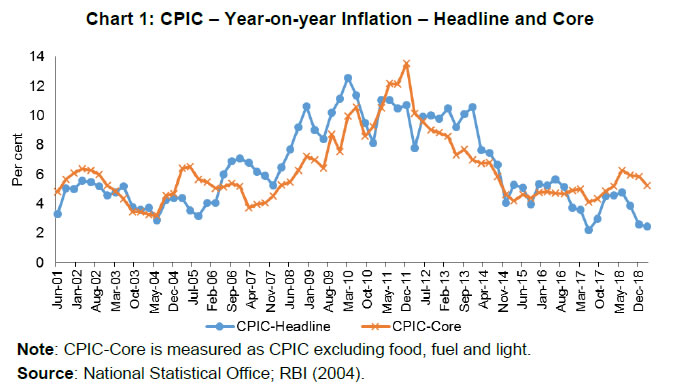

The RBI staff projections are based on a full information projection system that employs competing models such as structural time-series analysis and multivariate regression analysis, supplemented with inputs from forward looking surveys and lead indicators (Raj et al., 2019). The medium-term projections are generated from a quarterly projection model (QPM), which is a semi-structural, forward-looking, open economy, calibrated, gap model and captures key India-specific features such as food and fuel price dynamics and their spillovers onto other components of inflation and dynamics of inflation expectation formation (Benes et al. 2016). An evaluation of the RBI’s inflation projections indicates that the forecast errors were comparable to other countries. The modelling and forecasting approaches are constantly reviewed and refined by staff, and information collecting systems strengthened on an ongoing basis to minimise forecast errors (Raj et al., 2019).

IV. Empirical Results

Before proceeding to generate the forecasts from the individual models, all the variables used were tested for stationarity using Augmented Dickey Fuller (ADF) and Phillips Perron (PP) tests (Table 1).

Unit root tests suggest that all the variables used in the study, except call money rate and output gap (stationary in levels), are non-stationary at levels. Such non-stationary variables were transformed into stationary through first differences.

IV.1 Full Sample Analysis

We compare the forecasting performance, measured in terms of pseudo out of sample root mean squared error (RMSE)⁸ of individual models and their combinations relative to the performance of benchmark random walk model. Using the longer sample period (Q1:2001-02 to Q4:2018-19), the individual models were recursively estimated based on two different rolling windows viz. 24 and 32 quarters. Further, given the medium-term focus of monetary policy, the forecasting performance was examined for the horizon up to four quarters and the eighth quarter.

IV.1.1 Headline Inflation

Starting with headline inflation, and to illustrate in simple terms the relative performance of the alternative combination approaches, Chart 2 provides the comparison of forecasts of headline inflation generated from the individual models and forecast combination approaches vis-à-vis the actuals. More specifically, the pseudo out of sample forecasts up to four quarters ahead, generated in Q4:2015-16, Q4:2016-17 and Q4:2017-18, are compared with the actual inflation outturn.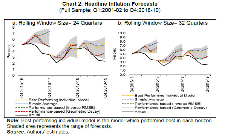

The RMSEs show that no individual model outperformed others across all the selected forecast horizons (Annex Table 1). However, the performance-based forecast combination consistently outperformed both the individual models as well as the simple average of the models. The performance-based forecast combinations outperformed even the ‘best’ individual model in the longer horizons (Chart 3).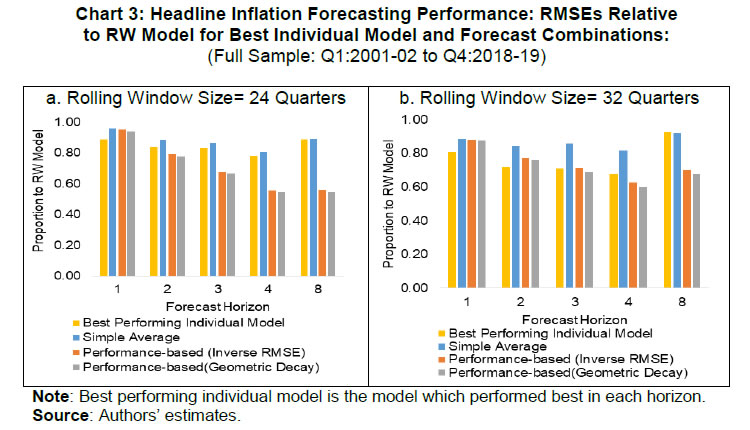

The relative forecasting performance improves considerably as the horizon is extended from one quarter to four quarters, a feature especially helpful from the monetary policy perspective, given the transmission lags. In case of the estimates with rolling window of 24 quarters, the RMSE of the performance-based forecast combination (with weighting scheme based on inverse weights), relative to the benchmark random walk model, was lower by 5 per cent and 44 per cent (against 4 per cent and 19 per cent in case of the simple average) for one quarter and four quarters ahead forecasts, respectively. A large improvement was also seen for the eight quarters ahead forecast vis-à-vis the benchmark model. The performance-based forecast combination with geometrically decaying weights was more or less similar with the forecast combination based on inverse RMSE weights (Annex Table 1).

For a formal statistical comparative performance of the three combinations, we use the Diebold-Mariano (DM) test to check whether combination forecasts generated using inverse RMSE and geometrically decaying weights significantly outperformed the simple average method over different forecast horizons (Table 2). For the first two cases in Table 2 comparing the simple average with the combinations, the null hypothesis is that the simple average is as good as the performance-based combinations against the alternate hypothesis that the simple average is less accurate than the other averaging methods. For the third case in Table 2 comparing the two combinations with each other, the null hypothesis is that the inverse RMSE based weighting is similar to weighting based on the geometric decay as against the alternate hypothesis that the inverse RMSE based weighting scheme is less accurate than the geometric decay based forecast combination. We use the modification suggested by Harvey, Leybourne, and Newbold (1998) to the DM test, which takes care of the problem with the assumption of zero covariance at 'unobserved' lags⁹. The results suggest that the performance-based weighting significantly improves upon the simple averaging method (Table 2).

A comparative assessment of the two performance-based combinations indicates broadly similar performance; at a few places, the geometric decay method though outperformed the RMSE based weighting scheme.

IV.1.2 Core Inflation

Turning to core inflation, Chart 4 provides a comparison of the forecasts generated using individual models and different combination approaches against the actual values. As in the case of the headline inflation, the analysis shows the superiority of the performance-based forecast combinations over individual models as well as the simple average approach. Moreover, as expected, the combinations do a much better job in forecasting relative to headline inflation. As core inflation is less volatile and more persistent, its forecasts are superior to headline inflation (RMSEs are lower for core inflation vis-à-vis headline inflation). Food, fuel and light have a share of 52.7 per cent in the CPIC basket in India and are subject to large and frequent supply shocks relative to core inflation. Sudden changes in the prices due to large and recurrent supply shocks could lead to a deterioration in the forecast performance of individual models; the relative performance of the individual models in such circumstances then perhaps changes more frequently as compared to the models for the more persistent core inflation. For a more formal analysis, we compare out of sample pseudo RMSE of the different forecasts.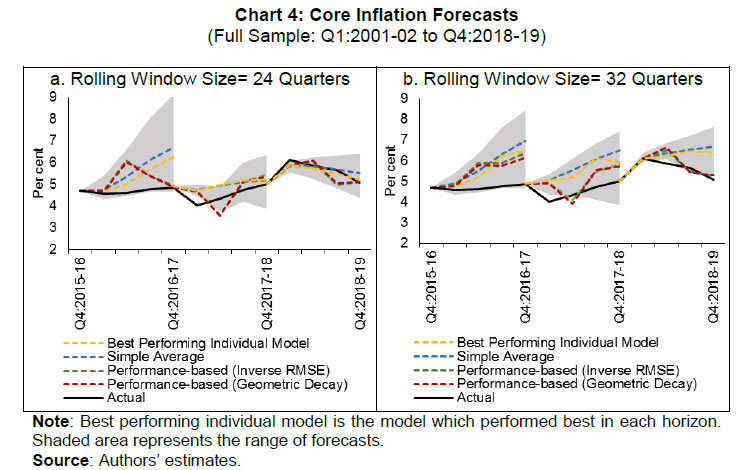

The comparison of the RMSEs indicates that the performance-based combination forecasts for core inflation (excluding food, fuel and light from the headline measure of inflation) outperformed the individual models and the simple average in the longer forecast horizons (Chart 5).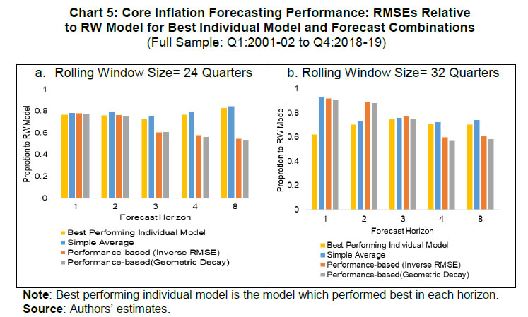

The simple average of the forecasts itself was able to better the benchmark forecast by 15-28 per cent across the four horizons and outperformed almost all the individual model-based forecasts. The performance-based forecast combination yielded even better results. For the 24 quarters window, the performance-based forecast combination was 22 per cent and 45 per cent better than the random walk model for one and four quarters ahead forecasts (Annex Table 2). Significant reduction in forecast errors was also observed in forecast combination, even for the eight quarters ahead horizon which is particularly relevant for the forward-looking monetary policy.

Like in the case of headline inflation, the DM tests show that at medium and longer horizons the performance-based forecast combinations are significantly better than a simple average of the individual models’ forecasts (Table 3). As in the case of headline inflation, for core inflation also the outcomes under the performance-based weights using inverse RMSE are broadly comparable to the geometric decay weights with a few exceptions. Unlike in the case of headline, for core inflation, the 8 quarters ahead forecast performance for the performance-based combination approaches was statistically superior to the simple average method.

IV.2 Trimming – Dropping the Underperforming Models

Following Bjornland et al. (2012), we assess the combination forecast performance by trimming the model space, i.e., by dropping certain underperforming individual models. Of the 26 models, 6 models (20 per cent of the models) with the highest RMSEs are excluded while combining the forecasts. The models were excluded for each horizon, looking at the ones with the highest RMSEs at respective horizons. The forecast performance of the trimmed models vis-à-vis the full set, given in Table 4, indicates that trimming does not make any material improvement to the forecast performance over various horizons and rolling window sizes. These results hold good for both headline and core inflation forecasts.

IV.3 Robustness Analysis

For robustness analysis, we restrict the sample period to Q1:2011-12 to Q4:2018-19 – a period for which the data are directly available from the official sources and hence do not require any backcasting. For this sample, we re-estimated the models and generated the individual forecasts as well as the forecast combinations. However, this shorter sample resulted in the loss of 40 observations, requiring a reduction in the rolling window sizes to 20 and 24 quarters for generating the combination forecasts so as to preserve sufficient data points for comparison across models. Furthermore, for the same reason, we only used a window of 4 quarters while estimating the performance-based measures. The results for this shorter sample period corroborate the findings of the full sample with greater force. For headline inflation, in the 24 quarters rolling window, the RMSE of the forecast combination (with inverse-weights) was 37-93 per cent of the benchmark RW model for the four forecast horizons for the shorter sample as compared with 56-95 per cent for the longer sample (Annex Table 3). Similar kind of conclusions can be drawn for the core inflation forecasts also. For core inflation, the RMSE of the forecast combination (with inverse-weights) was 21-81 per cent of the benchmark RW model for the four forecast horizons for the shorter sample as compared with 58-78 per cent for the longer sample (Annex Table 4).

IV.4 Comparison with Survey of Professional Forecasters

We now examine the performance of the forecast combination approach relative to the professional forecasters. Like other central banks, the RBI regularly conducts a survey of professional forecasters (SPF) wherein different professional forecasters give their individual projections for a set of macroeconomic indicators, including inflation. The results of the survey are published by the RBI in terms of mean and median of the individual forecasts – these results can, therefore, be interpreted as a variant of the simple average combination approach being studied in this paper. For professional forecasters, the available evidence for the US and the Euro area suggests that the simple average forecast of all the responses is the best combination and it is hard to find a combination that beats the simple average (D’Agostino et al., 2012; Meyler, 2020). Accordingly, an attempt is made to compare inflation forecasts (both for headline and core inflation) for the period Q1:2016-17 and Q4:2018-019¹⁰ for the unweighted combinations of SPF responses (mean and median) with the model-based combination forecasts – both unweighted and performance-based weighted – considered in this paper¹¹.

The results indicate that both mean and median forecasts of inflation from SPF have lower RMSEs than the simple average of individual model forecasts. The RMSE of the ‘best’ performing individual model seems to be more or less similar with the average SPF forecasts. The performance-based forecast combination of the models considered in this paper, however, outperformed the mean as well as median of SPF for both headline inflation and core inflation, especially, in the longer horizon (Chart 6). As fewer data points are available currently for this comparative analysis, it would be useful to revisit this analysis as more data become available.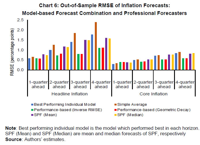

V. Conclusion

Inflation forecasts are the key inputs for monetary policy formulation by inflation targeting central banks. Inflation forecasting has become a more challenging task due to weakening of the traditional link between inflation and economic activity across countries for a variety of factors such as greater external openness, volatile exchange rates and commodity prices, increased competition from e-commerce, and potential non-linearities. In this milieu, a forecast combination approach – combining forecasts from alternative models through a judicious performance-based weighting system – can potentially enhance the forecasting performance of the individual models.

This paper empirically examined the forecasting performance of the combination approaches in the Indian context relative to a wide range of individual models spanning different modelling frameworks. Although the combination forecasts significantly improve upon the individual models, the absolute forecast errors of the combination models are non-negligible. A part of these errors is due to the large recurrent fluctuations in the key conditioning variables such as crude oil prices and exchange rate movements. Large shocks from the food side also contribute to the forecast errors. The other part of the error arises from model misspecifications and breaks in structural relationships, which can be addressed, to some extent, through forecast combinations, the subject matter of this paper. The empirical analysis showed that even the simple average of the forecasts based on individual models was comparable with the ‘best’ performing individual model’s forecast. The performance-based weighting schemes outperformed the individual models both for headline inflation as well as core inflation by a substantial margin at the longer horizons. The performance-based forecast combinations also turned out to be superior to the mean/median of the forecasts of the professional forecasters. Overall, the paper’s analysis shows that performance-based inflation forecast combinations can add value to the forecasting exercise; however, ongoing structural transformations, greater role of global factors including volatility in crude oil prices and exchange rates and weather shocks continue to pose challenges to the forecasting process.

* Corresponding author e-mail: joicejohn@rbi.org.in

^@ Joice John and Sanjay Singh are Assistant Advisers, and Muneesh Kapur is Adviser in the Monetary Policy Department, Reserve Bank of India.

¹ The views and opinions expressed in the paper are those of the authors and do not necessarily represent the views of the Reserve Bank of India. Comments from Himani Shekar and anonymous referee are gratefully acknowledged.

² There is a flurry of literature on combining models and/or forecasts for improving the performance. These can be broadly classified into model averaging and forecast combinations. The difference between averaging the models and the forecasts (i.e. the outcomes of the models) is that in the first case the models themselves gets combined and the forecast is generated and in the latter each of the models make individual forecasts and then the forecasts are combined. The focus of this paper is on forecast combinations.

³ Output gap is defined as (actual GDP level minus potential GDP level)*100/(potential GDP level). Potential GDP is estimated by using Hodrick-Prescott (HP) filter.

⁴ We use λ = 0.72 in the paper; this gives higher weights for the recent forecast performance.

⁵ We have used the Econometrics Toolbox by James P. LeSage for carrying out the estimation of the individual models (LeSage, 2005).

⁶ Back-casted data for CPI excluding food and fuel have been estimated following the approach in RBI (2014) for headline inflation, i.e. CPI-IW prices and the CPIC weights were used to calculate CPI excluding food and fuel.

⁷ The paper’s objective was to assess combination forecasts for up to 8 quarters. Such a medium-term forecast perspective necessitated the inclusion of GDP as an explanatory variable in a number of models to capture demand-supply conditions. Since GDP is available on a quarterly basis, the paper has focused on quarterly forecasts.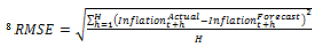

⁹ The Matlab routines provided by Trujillo (2020) have been used for this purpose.

¹⁰ Forecasting performance was evaluated for the period where common data is available. Hence, SPF results were compared with the models estimated for the shorter sample period, viz. Q1:2011-12 to Q4:2018-19. Since models were built based on the data for 20-quarters (i.e. rolling windows of 20-quarter), the forecasts become available only after 20-quarters. Hence, comparison of forecasts is done for the period Q1:2016-17 to Q4:2018-19.

References:

Aiolfi, M., & Timmermann, A. (2006). Persistence in forecasting performance and conditional combination strategies. Journal of Econometrics, 135(1-2), 31-53.

Bates, J. M., & Granger, C. W. (1969). The combination of forecasts. Journal of the Operational Research Society, 20(4), 451-468.

Behera, H., Wahi, G., & Kapur, M. (2018). Phillips curve relationship in an emerging economy: Evidence from India. Economic Analysis and Policy, 59, 116-126.

Benes, J., K. Clinton, A. George, P. Gupta, J. John, O. Kamenik, D. Laxton, P. Mitra, G. Nadhanael, R. Portillo, H. Wang, & Zhang, F. (2016). Quarterly projection model for India: Key elements and properties. RBI Working Paper Series No. 8.

Bjørnland, H. C., Gerdrup, K., Jore, A. S., Smith, C., & Thorsrud, L. A. (2012). Does forecast combination improve Norges Bank inflation forecasts? Oxford Bulletin of Economics and Statistics, 74(2), 163-179.

Clemen, R. T. (1989). Combining forecasts: A review and annotated bibliography. International journal of forecasting, 5(4), 559-583.

D’Agostino, Antonello, Kieran McQuinn and Karl Whelan. (2012). Are some forecasters really better than others? Journal of Money, Credit and Banking, 44(4), 715-732.

Dholakia, R., H., and V.S. Kadiyala. (2018). Changing dynamics of inflation in India. Economic & Political Weekly, LIII(9), 65-73.

Forbes, K. (2019). Inflation dynamics: Dead, dormant, or determined abroad? Working Paper No. 26496. National Bureau of Economic Research.

Gilchrist, S., & E. Zakrajsek. (2019). Trade exposure and the evolution of inflation dynamics. Finance and Economics Discussion Series. Washington: Board of Governors of the Federal Reserve System. https://doi.org/10.17016/FEDS.2019.007.

Harvey, D. I., Leybourne, S. J., & Newbold, P. (1998). Tests for forecast encompassing. Journal of Business & Economic Statistics, 16(2), 254-259.

Hibon, M., & Evgeniou, T. (2005). To combine or not to combine: selecting among forecasts and their combinations. International Journal of Forecasting 21, 15-24.

Hooper, P., Mishkin, F. S., & Sufi, A. (2020). Prospects for inflation in a high pressure economy: Is the Phillips curve dead or is it just hibernating? Research in Economics, 74(1), 26-62.

Hubrich, K., & Skudelny, F. (2017). Forecast combination for euro area inflation: A cure in times of crisis? Journal of Forecasting, 36(5), 515-540.

John, J. (2015). Has inflation persistence in India changed over time? The Singapore Economic Review, 60(04), 1550095.

Kapetanios, G., Labhard, V., & Price, S. (2008). Forecasting using Bayesian and information-theoretic model averaging: An application to UK inflation. Journal of Business & Economic Statistics, 26(1), 33-41.

Kapur, M. (2013). Revisiting the Phillips curve for India and inflation forecasting. Journal of Asian Economics, 25, 17-27.

LeSage, J. P. (2005). Econometrics toolbox for matlab. Internet site: http://www.spatial-econometrics.com/.

Litterman, R. B. (1979), Techniques of forecasting using vector autoregressions, Working Paper 115, Federal Reserve Bank of Minneapolis.

Litterman, R. B. (1980), A Bayesian procedure for forecasting with vector autoregressions, mimeo, Massachusetts Institute of Technology.

Makridakis, S., Spiliotis, E., & Assimakopoulos, V. (2020). The M4 Competition: 100,000 time series and 61 forecasting methods. International Journal of Forecasting, 36(1), 54-74.

Meyler, A. (2020). Forecast performance in the ECB SPF: Ability or chance? Working Paper 2371. European Central Bank.

Mishkin, F. S. (2007). Headline versus core inflation in the conduct of monetary policy. A speech at the Business Cycles, International Transmission and Macroeconomic Policies Conference, HEC Montreal, Montreal, Canada.

Mohanty, D., & John, J. (2015). Determinants of inflation in India. Journal of Asian Economics, 36, 86-96.

Mohanty, D., Chakraborty, A. B., Das, A., & John, J. (2011). Inflation threshold in India: An empirical investigation. RBI Working Paper Series, RBI WPS (DEPR): 18/2011.

Nachane, D. M., & Lakshmi, R. (2002). Dynamics of inflation in India -A P-Star approach. Applied Economics, 34(1), 101-110.

Nelson, C. R. (1972). The prediction performance of the FRB-MIT-PENN model of the US economy. The American Economic Review, 62(5), 902-917.

Öğünç, F., Akdoğan, K., Başer, S., Chadwick, M. G., Ertuğ, D., Hülagü, T., Kösem, S., Özmen, M.U., & Tekatlı, N. (2013). Short-term inflation forecasting models for Turkey and a forecast combination analysis. Economic Modelling, 33, 312-325.

Patra, M. D., Khundrakpam, J. K., & George, A. T. (2014, August). Post-global crisis inflation dynamics in India: What has changed? in Shah, Shekhar, Barry Bosworth and Arvind Panagariya (2014), India Policy Forum 2013-14, Vol. 10, Sage Publications, New Delhi, pp. 117-203

Patra, M. D., Khundrakpam, J.K, & John, J. (2018). Non-linear, asymmetric and time-varying exchange rate pass-through: Recent evidence from India. RBI Working Paper Series, RBI WPS (DEPR): 02/2018.

Pattanaik, S., & Nadhanael, G. V. (2013). Why persistent high inflation impedes growth? An empirical assessment of threshold level of inflation for India. Macroeconomics and Finance in Emerging Market Economies, 6(2), 204-220.

Raj, J., Kapur, M., Das, P., George, A.T., Wahi, G. & P. Kumar. (2019). Inflation forecasts: Recent experience in India and a cross-country assessment. Mint Street Memo No. 19, Reserve Bank of India.

Raj, J., Misra, S., George, A.T. & John, J. (2020). Core inflation measures in India – An empirical evaluation using CPI data. RBI Working Paper Series, RBI WPS (DEPR): 05/2020.

Reserve Bank of India. (2014). Report of the expert committee to revise and strengthen the monetary policy framework. URL: /documents/87730/39711208/ECOMRF210114_F.pdf

Reserve Bank of India. (2017). Monetary Policy Report, April.

Reserve Bank of India. (2019). Monetary Policy Report, April.

Reserve Bank of India. (2020). Monetary Policy Report, April.

Stock, J. H., & Watson, M. W. (2004). Combination forecasts of output growth in a seven‐country data set. Journal of forecasting, 23(6), 405-430.

Trujillo, J. (2020). dmtest_modified (e1, e2, h), MATLAB Central File Exchange. Retrieved May 3, 2020. (https://www.mathworks.com/matlabcentral/fileexchange/58787-dmtest_modified-e1-e2-h),

Zhang, B. (2019). Real‐time inflation forecast combination for time‐varying coefficient models. Journal of Forecasting, 38(3), 175-191.

Annex