Abhiman Das, Manjusha Senapati and Joice John*

Measurement of house price at an aggregate level poses several challenges. House prices vary significantly with associated quality attributes and in order to capture the true price change, the effect of quality of house should be adjusted appropriately. In this context, hedonic price index principle is a widely accepted method for quality adjustment. This paper attempts to construct hedonic price index by two different hedonic methods, viz., Time Dummy Method and Characteristics Price Index method, using survey data on rent and sale/resale prices of residential properties in Mumbai for the period January 2004 to November 2007. The results reveal that impact of quality adjustment is sizable and hedonic house price indices are much lower than traditional median weighted average price indices.

JEL Classification :   C43, C51, O18, R20

Keywords             :   House price, Hedonic, Price index

Introduction

House is a basic necessity of our life. Besides providing shelter, it is a major form of individual wealth. Understanding its price movements is important for a number of reasons. Changes in its value may influence consumer spending and saving decisions, which in turn affect overall economic activity. Changes in housing prices impact and reflect the health of the residential investment sector, a major source of employment. More importantly, many fundamental factors that shape the market’s expectations of future supply and demand relating to house price movements are not directly observable. As a result, it is difficult to ascertain whether rapid shifts in house prices are reflecting changes in the underlying fundamentals or not.

When the expectations turn out to be wrong or get revised as new information becomes available, real estate market witnesses dramatic adjustments in prices and this raises concern that prices have lost touch with the underlying fundamentals (Plosser, 2007). Therefore, from the Central Banks’ point of view, monitoring of house price movements is important for maintaining financial stability. In this context, it is essential to have accurate measure of aggregate housing prices.

As with many economic statistics, measurement of house prices also poses conceptual and practical problems. It is not easy to define ‘a house’ uniquely. Each house is associated with many quality attributes and thus making price comparison is difficult across units. Thus, standard index number theory is not applicable directly. The computation of a price index requires reliable data and a rigorous and robust methodology. The methodological problems associated with compilation of a housing price index are somewhat different from that of any standard price index: how is pure price evolution to be separated from changes in the quality of houses? First, for example, two houses are never exactly the same, because they have many characteristics, the unique combination of which translates into a particular housing service. Second, frequency of exchange of houses is much less than the other goods. These features lead to the problem of understanding the price evolution of a house or of a given group of dwellings, when very few prices are observed at each period. The observed transactions are few, and are a non-random sample of the housing stock. On the other hand, the housing stock itself is not fixed: it keeps changing through destruction, deterioration, improvement, new construction, extension, etc. Should the housing stock be perfectly fixed, transactions would have to be a large enough random sample of the housing stock to be validly used to compute price evolution. In addition, market does discount the age factor of the house in arriving at a price. Ideally the average price index should be a weighted average of prices of different ages and other characteristics. Thus the comparison of average sale prices is a mixture of true price evolution and change in the quality of the sample of transactions drawn from the stock. Further, house prices vary significantly with associated quality attributes like location, floor, facing side and many other facilities directly linked to standard of living. These are like add-on items; for every add-on item, there is an additional price. For all these reasons, the use of econometric techniques cannot be avoided. In the face of such challenges, different methodologies have been followed to measure aggregate price of housing. This paper attempts to estimate hedonic price index by two different methods using the data on sale/resale prices of residential properties in Mumbai based on a survey undertaken by Reserve Bank of India (RBI).

The paper is organised as follows. Section II presents a brief literature review, section III gives different methodologies of compilation of housing price index and section IV presents hedonic price index model used in the present study. Section V provides issues relating to house price measurement in India and presents a brief account of the overall residential property price movements in Mumbai based on the RBI survey results. Estimation and analysis is presented in section VI. Concluding remarks follow.

Section II
Literature Review

A price index intends to measure the effects of price changes over time while keeping other economic factors constant. Quality changes that take place over time in a rapid phase pose a fundamental problem in constructing a robust price index that measures only the pure price change over time. Separating pure price change and the quality change components from the total price change is a major challenge for the price index producer. Traditionally, several methods are available for quality adjustments. These include overlap pricing, direct quality adjustment using information from producers, and linking methods. But all these methods potentially suffer from subjective biases in selecting newly appeared products that most closely resemble the old ones.

Waugh (1928) and Court (1939) first used hedonic method to explain the relationship between price and quality characteristics. A more objective way of dealing with quality change as compared with these methods was recommended by the Price Statistics Review Committee (US) in 1961. This committee suggested that statistical agencies explore hedonic methods, referring to the major study on hedonic price index method and its application by Griliches (1961). Works of Griliches (1961) and Chow (1967) received much attention in the potential use of hedonics which were further supported by Lancaster (1971) and Rosen (1974). Triplett and McDonald (1977) studied hedonic quality adjustments to replacement items in the refrigerator price index. Diewert (2001) developed a consumer theory approach to hedonic regression as a simplification of Rosen’s (1974) theory.

Several European countries and countries like U.S. and Japan, have adopted hedonic regression methodology in their CPI quality control, particularly in areas where quality adjustment is proved to be difficult using traditional methods. The result has been quite successful in some areas like housing, electronic goods, computers, clothing and cars (Pakes, 2001; Bascher and Lacroix, 1999; Liegey and Shepler, 1999; Shiratsuka, 1999; Fixler et al, 1999; Okamoto and Sato, 2001).

As mentioned earlier, houses have various idiosyncratic characteristics, including location, size, number of rooms, occupancy, age, etc. This heterogeneity translates into different sub-markets, various turnover rates, and prices. It leads to difficulties in analysing housing prices which are less frequently observable. As between two sales, the value of a house, in the economic sense, cannot be given. It has to be estimated from a model of price. To estimate the value of the reference stock, econometric models are used relating prices (the log of the price per square metre) to the characteristics of the dwellings. Sutton (2002) studied the joint behaviour of house prices, national incomes, real interest rates and stock prices within the context of a simple empirical model. He identified the typical response of house prices to changes in a small set of key determinants.

Among official house price series, the Halifax House Price Index is the UK’s longest running monthly house price series with data covering the whole country going back to January 1983. The methodology is based on the hedonic approach to price measurement characterised by valuing goods for the attributes. In the case of housing, prices are supposed to reflect the valuation placed by a purchaser on the particular set of physical and locational attributes possessed by the property they wish to buy. Prices are disaggregated into their constituent parts using multivariate regression analysis. This permits the estimation of the change in average price from one period to another on a standardised basis. An obvious analogy can be drawn with the standard basket of goods used for calculating the retail price index.

The US Office of Federal Housing Enterprise Oversight (OFHEO) publishes the OFHEO HPI, a quarterly broad measure of the movement of single-family house prices. The HPI is a weighted, repeat-sales index, meaning that it measures average price changes in repeat sales or refinancing on the same properties. This information is obtained by reviewing repeat mortgage transactions on single-family properties whose mortgages have been purchased or securitized by Fannie Mae or Freddie Mac since January 1975. The HPI was developed in conjunction with OFHEO’s responsibilities as a regulator of Fannie Mae and Freddie Mac. It is used to measure the adequacy of their capital against the value of their assets, which are primarily home mortgages.

Section III
Methodology for Compilation of House Price Index

Like any other price index, house price index also captures the relative price movement of houses over two time periods. Methodology of compilation of housing price index for major developed countries is summarized in Table 1. There are mainly 4 different methods of price measurements, as discussed is the following section.

III.1 Median/mean transactions price:

The simplest measures of house prices use some indicator of central tendency from the distribution of prices for houses sold during a period. Since house price distributions are generally positively skewed (predominantly reflecting the heterogeneous nature of housing, the positive skew in income distributions and the zero lower bound on transaction prices), the median is typically used rather than the mean. Further, as no data on housing characteristics, other than the size of house or location of the house are required to calculate a median or mean, a price series can be easily compiled.

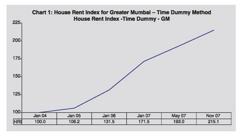
The main problem with median and mean prices is that they are subject to distortion by ‘compositional’ factors. Compositional factors include the volume of property sales within specific price bands. For example, if mainly low value properties in an area are sold in a month (and few of the superior properties in that area) then this can indicate a drop in the median or average. However, in the next month most sales in that area may be in superior properties (i.e., higher values) and this would then show that the median and average house price had increased when in fact overall values may have fallen. Median prices are affected by compositional change and seasonality. Hence, samples of observed transactions cannot be considered to be random. While median prices are widely used, alternative methodologies are employed in a number of countries to deal with the problem of compositional change and to obtain improved measures of housing prices.

III.2 Mix-adjusted

One means of controlling for changes in the mix of properties sold is to use the technique of stratification to construct a mix-adjusted measure of house prices. This is the methodology used by the Australian Bureau of Statistics (ABS) in its indices for established house prices. Mix-adjusted measures have also been used in a number of other countries including Canada, Germany and the United Kingdom, although there are differences between the approaches used in each country reflecting the diverse nature of housing markets across regions. In this method, typically, small geographic regions (e.g., suburbs) are clustered into larger geographic regions and then a weighted average of price changes in those larger regions is taken. Another approach along these lines uses price-based stratification, based on the evidence of marked compositional change between lower- and higher-priced suburbs. This appears to be highly effective in reducing the influence of compositional change. In particular, houses and societies sold in any period can be divided into groups (or strata) according to the long-run median price of their respective suburbs. The mix-adjusted measure of the city-wide average price change is then calculated as the average of the change in the medians for each group.

III.3 Repeat-sales

Rather than focusing on the price level in each transaction, this approach relies on the observed changes in price for those properties that have been sold more than once. It seeks to identify the common component in price changes over time. One limitation of a pure repeat-sales approach is that it uses only the data from those transactions involving properties for which there is a record of an earlier sale. An additional factor is that estimates of price changes in any quarter will generally continue to be revised based on sales that occur in subsequent quarters.

III.4 Hedonic method

In addition to repeat sales method, hedonic regression-based approaches have also been used by researchers and are used in the official measures produced in some countries, including the United Kingdom and United States. This method attempts to explain the price in each transaction by a range of property attributes, such as the location, type and size of a property, as well as the period in which it was sold. The resulting index of house prices can be thought of as the average price level of the transactions that occurred in each period, after controlling for the observable attributes of the properties that were sold. Hence, a hedonic approach can take account of shifts in the composition of transactions in each period. In principle, it can also control for quality improvements, although the ability to do so in practice depends on the comprehensiveness of data on housing characteristics.

Section IV
Hedonic Regression Model Specification

The hedonic method is basically a regression technique used to estimate the prices of qualities of an object. A hedonic price index is a price index that uses a hedonic function in some way. Four major methods, viz., time dummy variable method, characteristics price index method, hedonic price imputation method and hedonic quality adjustment method for calculating hedonic price indexes have been developed. Each of these four hedonic price index methods uses a different kind of information from the hedonic function. The first two methods (the time dummy variable method and the characteristics price index method) have sometimes been referred to as “direct” methods, because all their price information comes from the hedonic function; no prices come from an alternative source. Direct methods require that a hedonic function be estimated for each period for which a price index is needed. The next two hedonic price index methods (viz., the hedonic price imputation method and the hedonic quality adjustment method) have been described as “indirect” or “composite” methods. They are often called “imputation” methods, because the hedonic function is used only to impute prices or to adjust for quality changes in the sample in cases where matched comparisons break down. The rest of the index is computed according to conventional matched-model methods, using the prices that are collected in the usual sample.

In this paper, we use two direct methods, viz. Time Dummy Variable Index method and the Characristics Price Index method for constructing the house price index. These two methods are described in the following sections.

IV.1 Time dummy variable index method

A time dummy hedonic regression model is specified with the characteristics as independent variables and the natural log of the collected price as the dependent variable. Model specification for the time dummy method looks like this:

Whenever an item replacement takes place between the base and reference periods, quality change potentially occurs. The change in quality due to item replacement is taken care of by the associated characteristics, and the pure price change will be captured by the regression coefficient of the time dummy variable. The disadvantage of the time dummy variable index is that it is sensitive to specification bias and multi-collinearity.

IV.2 Characteristics price index method

An alternative approach for a comparison between price of houses in period t and t+1 is to estimate a hedonic regression for period t+1, and insert the values of the characteristics of modal house in period t into the period t+1 regression. This would generate predictions of the price of modal house existing in period t, at period t+1 shadow or implicit prices. This price can be compared with the price of the modal house in period t obtained from regression for period t.

Similarly another set of implicit prices could be generated by inserting the characteristics of modal house of period t+1 into the period t regression coefficients. This price is then compared with the price of the same modal house in period t+1 obtained from regression equation for period t+1.

The geometric mean of these two indexes gives us the desired characteristics price index. Let the regression equation for the period t be given as

In other words, this is nothing but the valuation of the typical base period (t) house by the current period’s implicit prices, obtained from the current period’s hedonic function, and compared with the same valuation for the base period. This is analogous to the Laspeyres type price index. Similarly the alternative index is the comparison of typical current period’s price with the hedonic function of the base period. The geometric mean of these two indexes would give the desired characteristics price index (Okamoto and Sato, 2001; Triplett, 2001).

Section V
House Price Measures in India

Until recently, India had no official system of collection and monitoring of real estate price movement. A proxy indicator in the form of rent is collected as a part of consumer price index. Both CPI(UNME) and CPI(IW) capture house rent price movements at half-yearly intervals. For CPI(UNME), apart from the middle class price collection data, a representative sample of rented dwelling occupied by non-manual employee families, the middle class house rent and middle class off-take are canvassed under the house rent and off take survey at the interval of six months for collection of comparable house rent data. For CPI(IW), the change in rent and related charges, which constitute a single item under housing group, is captured through repeat house rent surveys, which are conducted in the form of six-monthly rounds. This survey is conducted on a sub-sample of dwellings covered during the main income & expenditure survey in 1999-2000. The index is calculated once in every six months and is kept constant for the entire six months on account of the tendency of house rent to remain more or less stable over short periods. Under the house rent survey, three types of dwellings, viz. rented, rent free and self-owned are covered uniformly across all the centres. As the names suggest, both these indices capture house rent price movements for specific target population. Therefore, rent price movements based on these indices do not necessarily reflect true rent price movement of a city as a whole.

National Housing Bank, a government agency brought out an index of real estate price movements called Residex. It was developed based on a pilot study for five cities viz., Bangalore, Bhopal, Delhi, Kolkata and Mumbai for five years 2001-2005 (with 2001 as base). Later, Residex was extended to cover 15 cities and was updated up to (January-June) 2009 with base year as 2007. In terms of coverage, this index in the present form excludes price movements of commercial properties. Many private organisations also bring out synoptic view of real estate property price of selected cities in India.

To capture the data on rent and sale/resale price movements of residential as well commercial properties, the Reserve Bank of India conducted a pilot survey on real estate price movements of Mumbai as on January 2004, January 2005, January 2006, January 2007, May 2007 and November 2007. The weighted average price index of rent and sale/resale of houses in Mumbai, estimated from the price movements of individual transactions are presented in Table 2. The rent and sale/resale prices of residential properties in Mumbai have shown an unprecedented increasing trend over the years from 2004 to 2007. Monthly rent prices of residential properties in Mumbai had more than doubled during this period. During January 2004 to November 2007, median sale/resale price per sq. ft. of a standard apartment (500-1000 sq. ft.) showed an increase of 123.3 per cent and the same for large size apartment (>1000 sq. ft.) went up by 142.7 per cent. The price index of commercial sale/resale prices per sq. ft. had increased from 100 in January 2004 to 176 in November 2007. Intra-city variations in property prices in Mumbai were also found to be too large.

In the present paper, using the same data, we develop the hedonic price index for residential properties in Mumbai.

Section VI
Estimation and Analysis of Hedonic Regression

As indicated earlier, hedonic regression was estimated based on the data obtained from the RBI pilot survey conducted in 25 areas of Greater Mumbai during January 2004-November 2007 covering both residential and commercial properties. The actual transaction price, inclusive of land but exclusive of registration fee, stamp duty, brokerage fee, etc., was taken as the purchase price. The selection of sample in Mumbai was based on the municipal administrative zones. Six urban municipal administrative zones and six municipalities constituted the strata for selection of areas. In all 25 representative areas with high number of transactions were selected across the 12 areas (six zones + six municipalities) on the basis of their share in the total areas in zones. For proper representation, a total of 20 transactions per year in each of the 25 areas were captured. Thus, a sample of 500 transactions was collected as on January 2004, January 2005, January 2006, January 2007, May 2007 and November 2007. The information for each transaction within a particular area was classified according to whether it is a residential property or a commercial property. Within the residential and commercial property selected, the transactions were further classified into whether the property is used for rental purposes or is subjected to sale/resale in the time period under consideration.

Six quality attributes associated with price variations are considered in the hedonic model. These are: floor (F) in which house is situated; floor space area (FSA), number of rooms (R), number of bath rooms (B), whether it is sale or resale (S) and availability of lift (L). Classifications of these attributes are presented in Table 3. In the hedonic regression model, all the categories are represented by dummy variables. Apart from these attributes, dummy variables are used to represent separate areas (corresponding to 6 zones in Greater Mumbai, indicated by zone Z1 to Z6, and 6 municipalities,) and 6 time periods (T). The list of the areas under each zone and municipality is given in Table D1 in the Annex. As expected, there exists a large price disparity across zones. For example, the per square feet price in Malabar Hill, which comes under the zone 1, is expected to be much higher than any of the areas in the suburbs. Among the different zones in suburbs also, the house prices are expected to be heterogenous. Results of the hedonic regression method are presented separately for time dummy method and characteristics price method.

VI.1 Hedonic Index for Residential Properties: Time Dummy Method

VI.1.1. Rent

For obtaining the hedonic index using this method, the dependent variable is natural logarithm of per square feet rent. The regression coefficients obtained are presented in the Table A of Annex. It can be seen that all zones are having significantly higher rent compared to the average rent for zone 5. Further the rent of zone 1 is 7.3 times (exp(1.99)) than that of zone 5. Further, higher floors are found to have more rent, as coefficients corresponding to all floor categories are found to be significantly positive. As expected, larger floor space area leads to higher rent. The rent of two room houses is not significantly different from one room house. This can be viewed as the number of rooms being insignificant when considered independent of the floor space area. However, for the three room houses, rent is significantly higher. Rent in case of three bathroom house is also significantly different from one bathroom house.

The quality-adjusted index is calculated directly by taking the exponential of the time-dummy coefficient. The Table 4 gives price index for rented residential properties in Greater Mumbai with January 2004 as base. The hedonic rent index, taking into account the changes in attributes of residential properties was increasing on an average at the rate of 20 per cent per annum (Table 4). The index registered highest growth during January 2006 - January 2007 of 30.4 per cent. Afterwards, it decelerated. Chart 1 shows the house rent index using Time Dummy method for different areas of Greater Mumbai.

VI.1.2. Sale/Resale

Regression coefficients obtained are presented in Table B in Annex. Zones 1, 2, and 3 are having significantly higher price compared to the average price of zone 6. Further the price of zone 1 is 4.5 times (exp(1.50)) than that of zone 6. The zone 4 and zone 6 are found to be have no significant difference in their average house price. The price of zone 5 is found to be significantly lower than that of zone 6. As expected the first hand sale is priced significantly more than that of resale price. It is found that the higher floors are priced significantly more than that of ground floor. The larger area, as expected, is significantly priced more. It is found that number of rooms is related negatively to price and it is found to be significant for more than 3 rooms category. It can viewed as less price for more number of rooms for a given floor space area. Table 5 shows zone wise hedonic price indices for sale/resale of residential properties using time dummy method. During the four year period, viz., 2004-07, the index grew at an average rate of 18 per cent per annum. The growth rate of the index for zone 1 area was the highest (25 per cent per annum) whereas, for zone 6 area, it was the lowest (13 per cent). For zone 2 to zone 5, the price increase was in the range of 15-19 per cent per annum.

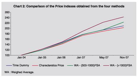
Table 6 shows hedonic index of sale/resale prices of residential properties in adjacent municipalities of Mumbai using time dummy method. The average rate of growth of index was highest in Badlapur (40 per cent) whereas it was lowest in Thane (9 per cent). Table C in Annex presents regression results for adjacent municipalities.

V. 2 Hedonic Price Index for Residential Properties: Characteristics Price Index Method

For calculating the index based on the characteristics price index method, we first identified the modal houses for different zones and different time periods. The modal values of the characteristics, viz., number of bathrooms, rooms, availability of lift, etc., are taken as the characteristics of the representative modal house in each zone for different time periods (Table E in Annex). The modal house is the most frequently transacted attribute of different characteristics in different zones during a particular period. The price movement of Mumbai city is estimated as the weighted average prices of 6 major tax zones (excluding municipalities), weights being the proportion of house stocks of the tax zones (Table D2 in Annex). The regression coefficients obtained are given in Table F of Annex. The relative price of zone 1, 2 and 3 with respect to zone 6 had been increasing steadily over the time points considered. This indicates the widening housing price gap between southern areas of Mumbai and its suburbs. The coefficients of zones 4 and 5 which are found to be negative in 2004 and 2005 became significantly positive in November 2007. This indicates that the price in zone 4 and 5 were less than zone 6 in 2004 and 2005, which had appreciated more and overtook zone 6 in 2007.

The Table 7 gives hedonic price index for residential properties in Mumbai using characteristics price index method. For residential properties of Mumbai using characteristic price index method, the average growth rate of index was around 17 per cent annum. Growth rate of house prices was highest for zone 1 areas (27 per cent) whereas it was lowest for zone 6 areas (9 per cent). For other areas of greater Mumbai, the growth rate was in the range of 12-20 per cent.

Table G in Annex gives regression results obtained for adjacent municipalities. In contrast to the coefficients of the zones in Greater Mumbai, the coefficients of adjacent municipalities tend to fall. This shows that the difference in house prices in the surrounding part of Greater Mumbai was decreasing. The Table 8 shows the price index for residential properties in adjacent municipalities of Mumbai using Characteristics Price Index method. The prices in adjacent areas of municipalities were growing at a higher rate than in the Greater Mumbai area. Growth rate in Badlapur municipality was the highest (44 per cent) whereas it was lowest in Thane (30 per cent).

Chart 2 gives comparison of price indexes obtained from the four different methods. The hedonic price indices are less as compared to other indices for the period under consideration. That is, price increase is subdued once the effect of quality attribute is controlled. This indicates that in order to asses the price movements of housing sector, quality attribute must be considered. The price indexes for greater Mumbai obtained from two hedonic methods, viz., time dummy and characteristic price method were moving together till January 2007. However, the index obtained from characteristic price method was moving slowly as compared to time dummy after January 2007.

Section VII
Conclusion

House is a major form of individual wealth. Understanding its price changes is important as changes in its value may influence consumer spending and saving decisions, and thus affect overall economic activity. From the Central Banks’ point of view, these are particularly important for maintaining financial stability. While it is important to have accurate measure of aggregate housing prices, its measurement poses significant conceptual and practical problems as each house is associated with many quality attributes which makes price comparisons difficult across units. Different methodologies have been followed to measure aggregate price of housing. This paper attempts to construct hedonic price index by two different methods, viz., Time Dummy Method and Characteristics Price Index method using the data on rent and sale/resale prices of residential properties in Mumbai for the period from January 2004 to November 2007. Results reveal that the price indices for Greater Mumbai obtained from the above-mentioned two methods were moving together till January 2007. However, the index obtained from characteristic price method moved slowly as compared to time dummy method after January 2007. The hedonic price indices are less as compared to other indices for the period under consideration. That is, price increase is subdued once the effect of quality attribute is controlled. This indicates that in order to asses the price movements of housing sector, effect of quality attributes must be considered.

References :

Bascher, J. and Lacroix T. (1999), “Dishwashers and PCs in the French CPI: Hedonic Modelling from Design to Practice”, presented at the Fifth meeting of the International Working Group on Price Indexes, Reykjavik, Iceland, August, 1999.

Chow, G.C. (1967), “Technological Change and the Demand for Computers”, American Economic Review 57, pp. 1117–1130.

Court, A. (1939), “Hedonic Price Indexes with Automotive Examples”, The Dynamics of Automobile Demand, pp.99-117, General Motors Corporation.

Diewert W.E. (2001), “Hedonic Regressions: A Consumer Theory Approach”, Discussion Paper, Department of Economics, University of British Columbia.

Fixler, D., Fortuna, C., Greenlees, J. and Wlater, L . (1999), “The Use of Hedonic Regressions to Handle Quality Change: The Experience in the US CPI”, paper presented at the Fifth Meeting of the International Working group of Price Indexes, Reykjavik, Iceland, August 1999.

Griliches, Z. (1961), “Hedonic Price Indexes for Automobiles: An Econometric Analysis of Quality Change”, The Price Statistics of Federal Government, New York, National Bureau of Economic Research.

Lancaster, K. (1971), “Consumer Demand: A New Approach”, Columbia University Press, New York.

Liegey, P.R. and Shepler, N. (1999), “Adjusting VCR Prices for Quality Change: A Study Using Hedonic Method”, Monthly Labour Review.

Melser, D. (2005), “The Hedonic Regression Time-Dummy Method And The Monotonicity Axioms”, Journal of Business & Economic Statistics, 23(4): 485-492.

Okamoto, M. and Sato, T. (2001), “Comparison of Hedonic Method and Matched Models Methods using Scanner Data: The Case of PCs, TVs and Digital Cameras”, Paper presented at the Sixth Meeting of the International Working Group on Price Indexes, Canberra, Australia, 2-6 April 2001.

Pakes, A. (2001), “A Reconsideration of Hedonic Price Indexes with an Application to PC’s”, NBER working paper 8715, Cambridge MA.

Plosser, C. I. (2007), “House Prices and Monetary Policy”, Speech by the President, Federal Reserve Bank of Philadelphia, European Economics and Financial Centre, Distinguished Speakers Series.

Rosen, S. (1974), “Hedonic Prices and Implicit markets: Product Differentiation and Pure Competition”, Journal of Political Economy, 82, 34-49.

Shiratsuka, S. (1999), “Asset Price Fluctuation and Price Indices”, Monetary and Economic Studies.

Sutton, G. (2002), “Explaining Changes in House Prices”, BIS Quarterly Review.

Triplett, J. E (2001), Handbook on Quality Adjustment of Price Indexes for Information and Communication Technology Products, Paris: OECD.

Triplett, J.E., and McDonald R.J. (1977), “Assessing the Quality Error in Output Measures: The Case of Refrigerators”, The Review of Income and Wealth, 23, 137-156.

Waugh, Frederick, V. (1928): “Quality Factors Influencing Vegetable Prices”, Journal of Farm Economics, 10,185-196.

* Dr. Abhiman Das is Assistant Advisor and Smt. Manjusha Senapati and Shri Joice John are Research Officers in the Department of Statistics and Information Management. The views expressed in the paper are strictly personal.