by Joice John, Deepak Kumar, Asish Thomas George, Pratik Mitra, Muneesh Kapur and Michael Debabrata Patra^{^}

The recalibrated quarterly projection model (QPM 2.0) presented in this article is a forward-looking open economy gap model calibrated to generate forecasts, undertake risk assessment and provide policy analysis for the Indian economy. QPM 2.0 augments QPM 1.0 with fiscal-monetary policy interaction, a more nuanced modelling of domestic fuel pricing dynamics, capital flows, exchange rate dynamics and central bank’s forex market interventions for a more informed judgement.

The Reserve Bank of India (RBI)’s Quarterly Projection Model (QPM) is a calibrated, forward-looking, open economy, new-Keynesian gap model incorporating specific characteristics of the Indian economy. Its main purpose is to generate medium-term projections and policy analysis consistent with achieving targets/mandate set under the flexible inflation targeting (FIT) framework. The documentation of its predecessor, i.e., QPM version 1 (QPM 1.0) was published in 2016 (Benes et al., 2016a; b). Armed with the lessons of experience, since then, the model structure and parameters were recalibrated to enhance the model with more India-centric characteristics in order to enrich its performance and relevance.¹

The major enhancements brought about in version 2 (QPM 2.0) are as follows:

1. fiscal-monetary policy interaction;

2. domestic fuel pricing dynamics (oil prices, exchange rates and fuel taxes);

3. capital flows and exchange rate dynamics; and

4. re-parametrisation, incorporating data till Q4:2019 (pre-COVID period)².

The rest of the article is arranged into six sections. Section II provides the model structure. The equations and approach to calibration are explained in section III. Model properties in terms of impulse response functions (IRF) are described in section IV. Historical decompositions of major macroeconomic variables are discussed in section V. Section VI presents forecast performance and Section VII concludes.

II. Model Structure

QPM 2.0 embodies the standard new-Keynesian small open-economy framework. It has 6 blocks, viz., i) an aggregate demand block comprising the output gap and credit conditions; ii) an aggregate supply block modelling inflation, inflation expectations and central bank credibility; iii) short-term interest rates (policy reaction function and operating target) and transmission to long-term interest rates; iv) fiscal block; v) the exchange rate via the modified risk-adjusted uncovered interest parity condition, capital flows and forex market intervention; and vi) foreign sector block (Chart 1).

II.1. Fiscal-Monetary Policy Interaction

Fiscal policy dynamics can have sizeable effects on output and inflation. Therefore, appropriate modelling of monetary and fiscal policy interaction is vital for improving the understanding of output and inflation behaviour in the context of attaining price stability and sustained growth (Woodford, 2001; Canzoneri et al. 2011). Hence, the overall fiscal deficit is decomposed into the primary deficit and interest payments. The primary deficit has structural (cyclically adjusted) and cyclical (automatic stabilisers) components. The cyclical component is modelled as a function of the output gap. Unanticipated changes in the structural deficit in the form of government consumption impacting private consumption and thereby domestic economic cycles form fiscal impulses (Blanchard and Perotti, 2002). Debt dynamics incorporate a) the relationship between debt and the overall fiscal deficit and b) the overall deficit that is compatible with a sustainable level of debt (Escolano, 2010). The steady state structural deficit is linked to the steady state debt level and nominal output growth. Deviations from the long-term debt target affect the country risk premium and the exchange rate through the modified risk-adjusted uncovered interest parity (MRUIP) condition. Changes in aggregate demand and the exchange rate affect inflation, leading to changes in monetary policy. At the same time, monetary policy affects the fiscal deficit through interest payments – short-term interest rate affects long-term rate.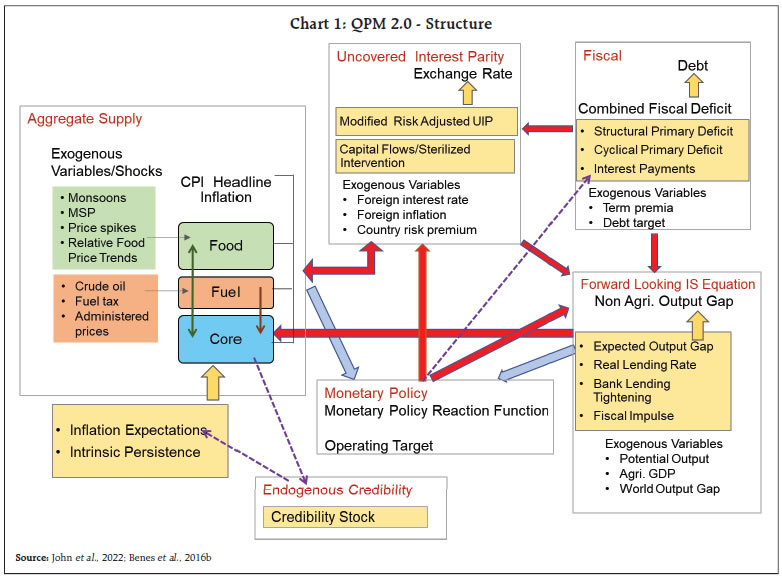

II.2. Fuel Pricing

India has a distinctive system of fuel pricing. Some components of fuel consumption like petrol and diesel are priced on the basis of market variables – international crude oil prices and exchange rates. Some items like liquefied petroleum gas (LPG) and kerosene are market determined but with a lagged pass-through. Prices of another set of fuel items like electricity are administered. Prices of petrol and diesel include a substantial portion of non-ad valorem taxes, which impedes the full pass-through of crude oil price changes to inflation. Considering these factors, the fuel section has three different components: a) ‘market fuel 1’, comprising petrol and diesel prices, is determined by changes in crude oil prices, exchange rates and fuel taxes (excise duty and VAT); b) ‘market fuel 2’ consisting of LPG and kerosene for which prices are determined by international fuel prices and exchange rates, but with a lag; and c) ‘administered fuel’ i.e., electricity and other items in the fuel and light subgroup of the CPI. Fuel prices have a substantial role in determining input cost pressures in the economy, which are modelled through spillovers from fuel to non-fuel components of inflation.

II.3. Capital Flows and Exchange Rate Dynamics

The standard approach to capital flows, exchange rates and monetary policy dynamics is based on the ‘trilemma’ (Mundell, 1963; Fleming, 1962). This was further developed into the new-Keynesian open economy framework, incorporating implications of global financial cycle and dominant currency paradigm (Obstfeld and Rogoff, 2000; Galí and Monacelli, 2005; Gopinath et al. 2020; Miranda-Agrippino and Rey, 2022). Volatility in capital flows and exchange rates has implications for macroeconomic management. The orthodox view holds that successful inflation targeting (IT) requires a high degree of exchange rate flexibility. In the context of emerging market economies (EMEs), however, it is observed that it is sub-optimal to overlook the costs associated with volatility in exchange rates due to sudden surges or reversals in capital flows.³ This has prompted many EMEs to adopt policy tools like forex market interventions for managing exchange rate volatility even under an IT framework (RBI, 2021).

III. Key Behavioural Equations and Calibration

QPM 2.0 has 154 equations (including identities), of which 57 are behavioural equations (Table 1).

III.1. Aggregate Demand: A Forward-Looking IS Curve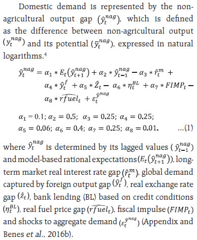

III.2. Aggregate Supply: Inflation

Considering the unique characteristics of inflation dynamics in India, separate equations are formulated for food, fuel and core⁵ components (analogous to the structure of QPM 1.0) (Benes et al., 2016b).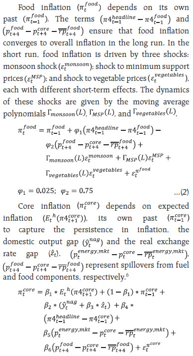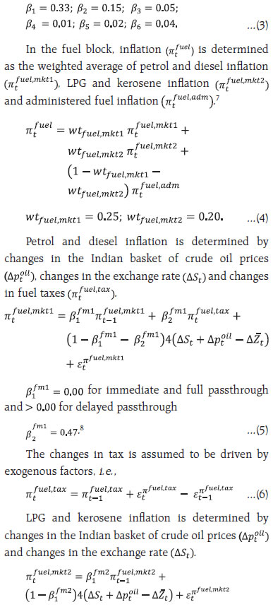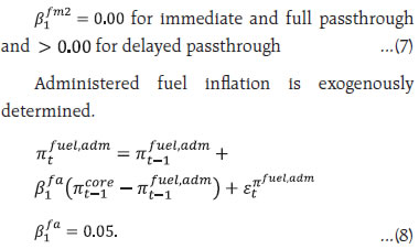

III.3. Interest Rates Block

The monetary policy repo rate equation follows an inflation forecast-based Taylor-type reaction function with an interest rate smoothing parameter (Benes et al., 2016b).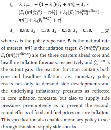

QPM 2.0 incorporates an additional equation for the operating target of monetary policy – weighted average call money rate (WACR) – as follows: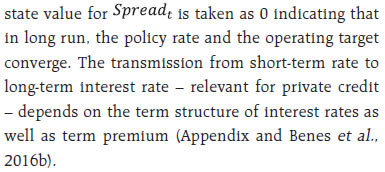

III.4 Fiscal Block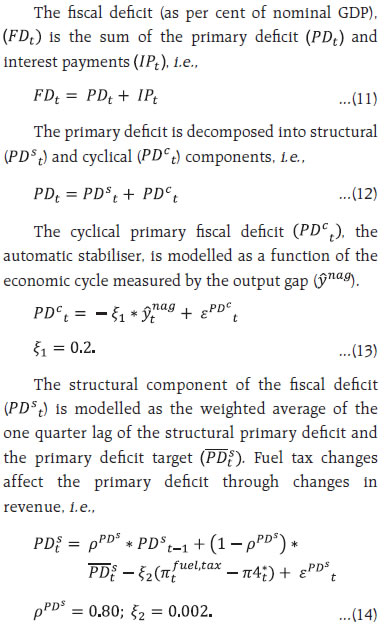

The primary deficit target is calibrated in line with the Fiscal Responsibility and Budget Management (FRBM) path of fiscal consolidation:

Deviations of the structural primary deficit from its target capture fiscal impulse (FIMP_t):

Debt accumulation dynamics is modelled as follows: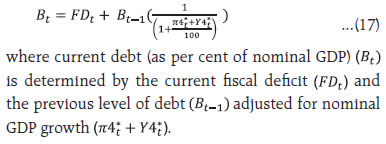

The steady state fiscal deficit (FD*) is related to steady debt dynamics (B*) as follows: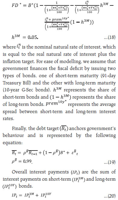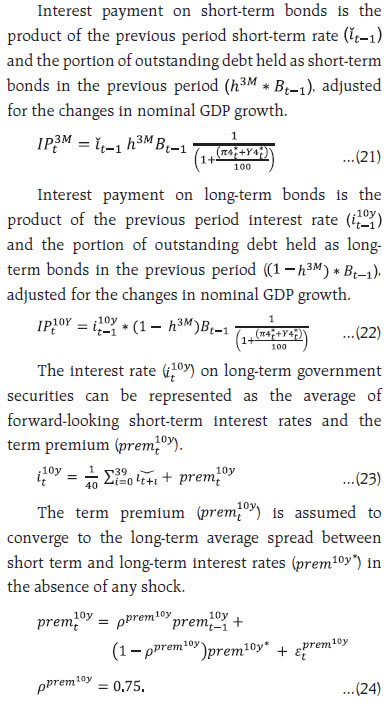

III.5 Modified Risk-adjusted Uncovered Interest Parity (MRUIP)

The uncovered interest rate parity (UIP) condition, wherein interest rate differentials determine the expected exchange rate, has been popularly used in small open economy models for monetary policy analysis. However, the UIP relation has been consistently and decisively rejected in the data (see Froot and Thaler, 1990; Lewis, 1995 and Engel, 1996 for comprehensive surveys). To reflect this empirical disconnect, time varying country risk premia and purchasing power parity conditions are introduced to moderate the effects of interest rates on exchange rates (Benes et al., 2016b).

Exchange rate dynamics captured through the MRUIP equation have been modified to incorporate features of external sector: a) an adjustment process for capital flows; b) determinants of current account; c) the balance of payments identity relating the current and capital accounts to the accumulation of reserves; and, d) forex interventions.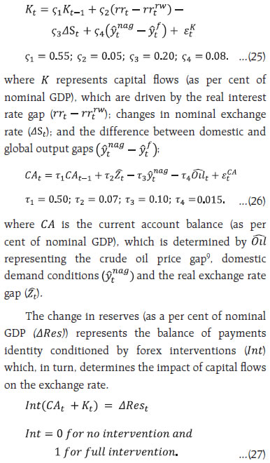

Incorporating the added features, the MRUIP equation is expressed as follows: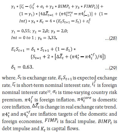

III.6. Foreign Block

The foreign block in QPM has two parts – the United States (US) block and rest of the world (RoW) block. The US block is a barebone new-Keynesian model with three behavioural equations – the IS curve, the Philips curve and the Taylor rule: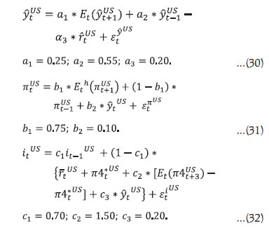

The RoW section of the foreign block incorporates an exogenous equation for crude oil price movements. The forecasts of foreign variables are exogenously provided, based on the information available from agencies like the United States Federal Reserve (US Fed), the International Monetary Fund (IMF) and the International Energy Association (IEA).

III.7. Calibration

The calibration of parameters of QPM 2.0 has been carried out through multiple iterations (Chart 2). This process includes a) generating econometric estimates by using linear regression models, non-linear regression models and vector auto regression (VAR) models; (b) using estimates from other empirical studies (Khundrakpam and Jain, 2012; Misra and Trivedi, 2016; Behera et al. 2017; Patra et al., 2018; Kapur, 2018; RBI, 2018; Goyal and Parab, 2019; Raj et al., 2018; RBI, 2019; Patra et al., 2021; Pattanaik et al., 2022); and (c) evaluating the fit by using model generated IRFs, historical decompositions and rolling forecasts.

Model solutions, simulations, historical decompositions and forecasts are carried out using the IRIS toolbox in MATLAB through following steps. First, the model needs to be linearised around a steady state. Second, dynamic solutions involving the forward-looking variables have to be obtained. Third, unobserved variables have to be filtered out from the state-space representation. Fourth, forecasts and policy simulations have to be generated.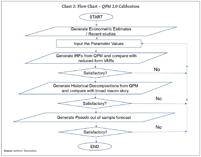

Steady states are computed by using a nonlinear Newton-type algorithm. The dynamic model solution is obtained from a nonlinear particle swarm optimizer (PSO), and a generalised Schur decomposition is used to integrate future expectations. The unobserved variables are filtered out by employing a multivariate Kalman filter (MvKF) with an exact nonlinear prediction step. The simulations generated from the model are based on a first-order approximate solution calculated around the steady state. The forecasts are generated by applying equation-selective nonlinear simulator with shanks acceleration.

IV. Model Simulations

IV.1. Output Gap (Demand) Shock

A positive demand shock of 1 percentage point (ppt) increases core inflation by 20 basis points (bps) at its peak. Headline inflation increases by around 20 bps. Both the output gap and the deviation of inflation from its target require an increase in the real interest rate, which is achieved through a hike in the policy interest rate. These changes dampen demand and over the medium-term, output returns to its potential level. With the elimination of excess demand, inflation returns to the target and all the real variables return to their long-term equilibrium (Chart 3).

IV.2. Core Inflation (Cost-push) Shock

A cost-push shock to core inflation presents monetary policy with a difficult trade-off. The policy rate has to be increased to ensure that inflation returns to target in the medium-term, but this opens up a negative output gap (Chart 4). With the unwinding of the interest rate as inflation falls to target, the output gap closes and output returns to its potential level.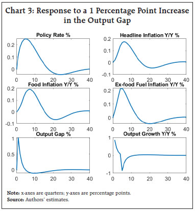

IV.3. Policy Rate Shock

A policy interest rate increase by 1 percentage point results in a fall in domestic demand by around 20 bps and a negative output gap opens up (Chart 5). Along with anchoring of inflation expectations and enhanced central bank credibility, this leads to a decline in core inflation by around 25 bps and headline inflation by around 20 bps. These effects, however, hold only in the short run. Over time, as inflation returns to the target, the interest rate decreases, which closes the output gap and neutralises the disinflationary effect of the initial interest rate increase.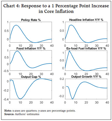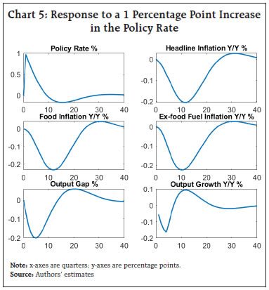

IV.4. Exchange Rate Shock

A depreciation in the exchange rate by 1 per cent leads to increase of around 7 bps in inflation via an exchange rate pass-through (ERPT) of 7 per cent (Chart 6). The output gap initially increases as a result of gains in external competitiveness. The increase in inflation and the output gap warrants monetary tightening. This leads to undershooting of the output gap, creating negative growth responses in the medium-term.

IV.5. Crude Oil Price Shock

An increase in global crude oil prices has direct effects on petrol, diesel, LPG and kerosene prices. The increase in market fuel prices induces a cost push shock and core inflation goes up. Higher crude oil prices also induce depreciation of the Indian Rupee (INR). This will have additional second round effects on inflation. Together, an increase in crude oil price by 10 per cent results in inflation increasing up by 30 bps at its peak (Chart 7). Aggregate demand slows down as firms take a hit on their profit margins, cash flows and investment. The increase in inflationary pressures, however, warrants a monetary policy response to bring inflation back to target.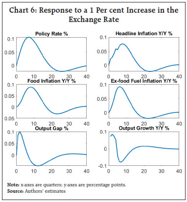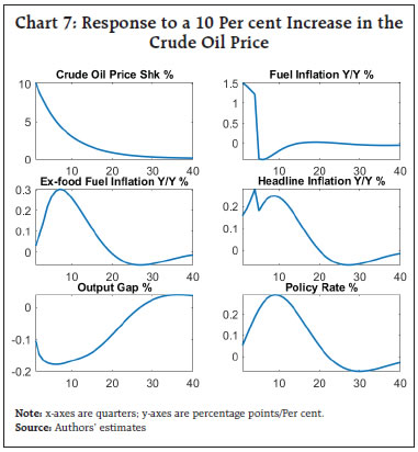

IV.6. World Output Gap (Demand) Shock

An increase in world demand by 1 percentage point leads to increase in domestic demand by 30 bps (Chart 8), which pushes up inflation. The increase in world demand also raises international crude oil prices. With India being an importer of crude oil, the higher crude oil prices exert additional pressure on headline and core inflation. The increase in domestic demand and inflation warrants tightening of monetary policy.

IV.7. Fuel Tax Shock

Fuel tax increases are sporadic and non-mean reverting. Hence, in QPM 2.0, the shocks to fuel taxes are assumed not to revert to their original values unless and until they are reversed exogenously. An increase in the fuel tax by ₹10 per litre leads to an increase in fuel prices and hence core inflation through the cost push channel. Inflation goes up by 25 bps (Chart 9). Inflationary pressures remain entrenched in the system due to the non-reversal of the increases. Demand conditions also remain subdued for a longer period for the same reason. The policy rate needs to increase to anchor inflationary expectations and neutralise second-round effects.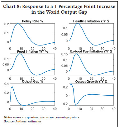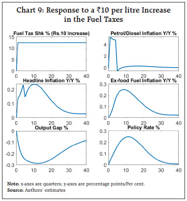

IV.8. Structural Primary Fiscal Deficit Shock

An increase in the structural primary fiscal deficit by 1 percentage point of GDP contributes to demand and opens up a positive output gap (Chart 10). The overall fiscal deficit goes up by the same amount, leading to accumulation of debt, which contributes to depreciation of the INR through country risk premium. The positive output gap and currency depreciation lead to higher inflation, warranting monetary policy action.

IV.9. Capital Flow Shock

The impact of capital flow shock (one percentage point of GDP) is conditional on the RBI’s decision to intervene and sterilise. In case of a capital outflow shock, assuming the RBI intervenes and sterilises 70 per cent, the reserves will deplete by 0.7 percentage point of nominal GDP. In this scenario, the exchange rate could depreciate by close to 1 per cent, inducing inflation of around 10 bps (Chart 11).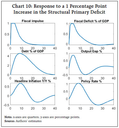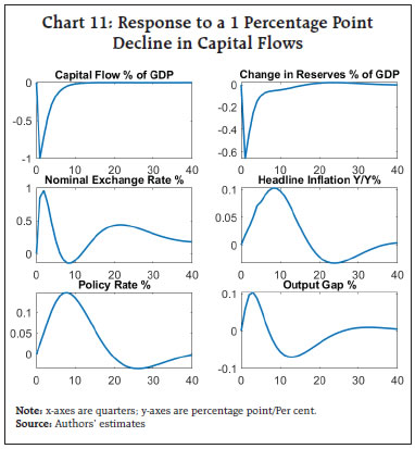

If the central bank decides not to intervene, there will be no depletion of reserves; however, the depreciation could be higher, leading to higher inflation and higher policy rates and imparting volatility to the exchange rate, inflation and policy rate. On the other hand, if the central bank chooses to intervene fully, an equal amount of reserves will be depleted and the exchange rate will remain more or less unchanged, warranting no monetary policy rate changes but with volatility in reserves.

V. Historical Decompositions

A historical decomposition (HD) of the major macro variables for the period 2011-2022 helps to understand the role of various shocks and policies in driving the trajectory of macroeconomic developments.

V.1. Headline Inflation

Prior to 2014 – the period which laid down the initial conditions of the FIT – headline inflation was in double digits. Food price shocks emanating from the monsoon and MSP, the lack of a nominal anchor, exchange rate depreciation and high fuel prices drove inflation up during that period (Chart 12). During 2014 to 2016, when a de facto FIT framework was pursued, the factors that contributed to high inflation during the pre-2014 period dissipated. Cost push shocks became disinflationary on the back of benign global commodity prices and exchange rate stability was restored as the external environment turn favourable. From 2014 onwards, fuel taxes started to contribute positively to inflation, offsetting the negative impact of the crude oil price decline. Owing to these factors, inflation steered close to 4 per cent by the time FIT was institutionalised in 2016.

From 2016 onwards, the nominal anchor set out by the FIT contributed favourably to inflation. Fiscal prudence also contributed to the disinflationary process. Up till Q3:2019, food price shocks led to a fall in inflation. Fuel price shocks were also favourable during this period.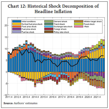

During the 2020-22 period, food price and cost-push shocks emanating from persistent supply chain disruptions due to the COVID pandemic and the war in Ukraine exerted upside pressure on headline inflation, partly offset by subdued demand conditions.

V.2. GDP Growth

The HD of GDP growth suggests that potential output shocks and structural factors were mostly responsible for the GDP growth slowdown during 2016-19 (Chart 13). The pandemic induced lockdown, supply chain bottlenecks and weak external demand adversely impacted domestic output and demand during 2020-22.

V.3. Policy Repo Rate

In the 2014-16 period, the stability in the exchange rate, favourable cost-push shocks and a conducive external environment contributed negatively to the policy rate. During the FIT period (2016 -2019), favourable food and fuel price shocks, external developments and fiscal prudence supported a lower policy rate environment (Chart 14). Most interestingly, the nominal anchor set out by the FIT contributed negatively to the policy rate during this phase. In other words, in the absence of a nominal anchor, the policy rate could have been higher in order to achieve the same level of inflation. This indicates that with an explicit nominal anchor, the monetary policy rates can afford to be raised less than otherwise for disinflating the economy.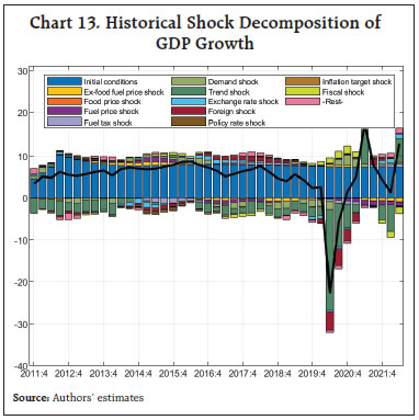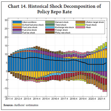

During 2020-22, a large negative output gap due to the pandemic caused monetary policy to follow an accommodative stance. From May 2022, the policy repo rate has been increased in a calibrated manner in view of headline inflation ruling above the target along with elevated core inflation.

V.4. Core Inflation

HD of core inflation is similar to that of headline inflation. The institution of the FIT regime, benign crude oil prices, fiscal prudence and favourable external environment provided cushions to core inflation during 2016-19, which more than offset the upside pressures from the increase in fuel taxes (Chart 15). Pandemic induced supply chain disruptions and cost push shocks led to elevated core inflation in 2020-22.

VI. Forecast Performance

This section evaluates the forecast performance of QPM 2.0 by generating pseudo out-of-sample forecasts of up to 8 quarters ahead and calculating the pseudo out-of-sample root mean square errors (RMSE) of major macroeconomic variables for the period from 2011 to 2019 (Chart 16).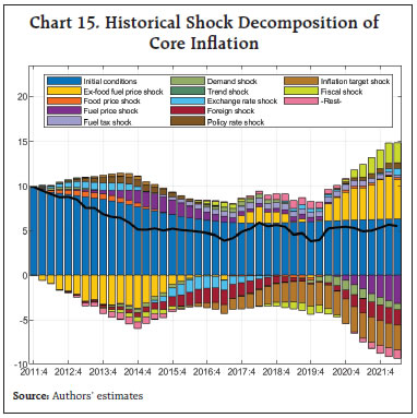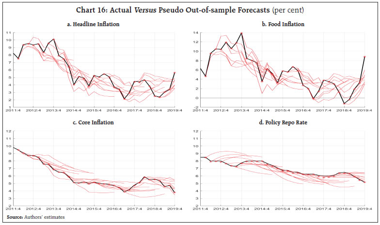

The hairline charts indicate that the forecasts of food inflation and headline inflation appear to be directionally consistent. Core inflation and policy rate forecasts seem to be less noisy than food and headline inflation forecasts.

A formal evaluation of the forecast is conducted by generating the pseudo out-of-sample RMSEs over various forecast horizons (Table 2).

The RMSEs of the headline inflation forecasts in the short to medium horizon (1-4 quarters) are marginally higher than that of time series forecasts and are comparable with that of the Survey of Professional Forecasters (SPF) (John et al., 2020; Raj et al., 2020). RMSEs of the best time series forecasts are 0.2 to 0.6 percentage points lower in 1-4 quarters. This behaviour is expected as large macroeconomic models tend to produce larger errors in the short-term relative to models based on time series and full information matrices. This is also the reason why the QPM uses forecasts from short-term forecasters as its initial condition. The forecast performance substantially improves in the medium horizon (5-8 quarters), which matters for the monetary policy decision. In the eight-quarter ahead forecasts, QPM turns out to be better than time series models (John et al., 2020) by a substantial margin.

The RMSEs of core inflation forecasts are substantially lower than that of the headline inflation, as expected. As in the case of headline inflation, RMSEs of core inflation forecasts from QPM are higher than time series forecasts and comparable to SPF forecasts over the 1-4 quarter horizon (John et al., 2020). In the medium horizon, however, QPM 2.0’s forecast accuracy is better than time series model forecasts (John et al., 2020) by considerable margins.

VII. Conclusion

Given the transmission lags which characterise the impact of monetary policy on output and inflation, forward-looking responses to expected inflation and output are warranted to maximize welfare. Both inflation and output are also shaped by expectations of future interest rates, as also inflation expectations of households and firms. Thus, inflation and output are the outcome of a complex web of interactions and feedback mechanisms in the economy. Accordingly, consistent and reliable forecasts of inflation and output are important as they assume the role of intermediate target of monetary policy. It is in this context that theoretically consistent and empirically well-founded models adapting country-specific features are at the heart of monetary policy formulation among modern central banks.

In India, the adoption of a flexible inflation targeting framework has been underpinned by a Quarterly Projection Model, which fulfils the requirement set out in Section 45ZM of the RBI Act of setting out inflation forecasts for 6-18 months in a half-yearly Monetary Policy Report (MPR).

QPM 2.0 takes that endeavour to the next level by enriching the existing new- Keynesian monetary model (QPM 1.0) with fiscal-monetary policy interactions, a more nuanced modelling of India-specific fuel pricing, capital flows, exchange rate dynamics and central bank’s forex market interventions. The QPM 2.0 thus takes monetary policy modelling closer to a general equilibrium framework that is more representative of India’s macroeconomic dynamics and helps to generate internally consistent forecasts and policy scenarios. This provides policymakers with relevant information and scenarios for a more informed judgement.

Historical decompositions generated from QPM 2.0 show that the inflationary surge in the wake of the pandemic and the war in Ukraine was triggered by successive supply shocks but as their impact waned, rising demand unleashed by the strengthening domestic recovery enabled pass-through of pent-up input costs, adding persistence to elevated inflationary pressures (Patra et al., 2022). The disinflation strategy adopted during this period has been strongly supported by improved precision in forecasts generated by QPM 2.0 relative to competing models.

References

Behera, H. K., Pattanaik, S., & Kavediya, R. (2017). Natural interest rate: Assessing the stance of India’s monetary policy under uncertainty. Journal of Policy Modeling, 39(3), 482-498.

Benes, M.J., Clinton, K., George, A., John, J., Kamenik, O., Laxton, M.D., Mitra, P., Nadhanael, G.V., Wang, H. & Zhang, F. (2016a). Inflation-forecast targeting for India: An outline of the analytical framework. RBI Working Paper Series No. 7/2016.

Benes, M.J., Clinton, K., George, A., Gupta, P., John, J., Kamenik, O., Laxton, M.D., Mitra, P., Nadhanael, G.V., Portillo, R. and Wang, H. (2016b). Quarterly projection model for India: Key elements and properties. RBI Working Paper Series No. 8/2016.

Blanchard, O., & Perotti, R. (2002). An empirical characterization of the dynamic effects of changes in government spending and taxes on output. the Quarterly Journal of economics, 117(4), 1329-1368.

Blanchard, O., Ostry, J. D., Ghosh, A. R., & Chamon, M. (2016). Capital flows: expansionary or contractionary?. American Economic Review, 106(5), 565-569.

Canzoneri, M., Cumby, R., & Diba, B. (2010). The interaction between monetary and fiscal policy. Handbook of monetary economics, 3, 935-999.

Fleming, J.M. (1962). Domestic Financial Policies under fixed and under floating exchange rates. Staff Papers-International Monetary Fund, 369-380.

Engel, C. (1996). The forward discount anomaly and the risk premium: A survey of recent evidence. Journal of empirical finance, 3(2), 123-192.

Escolano, J.(2010). A practical guide to public debt dynamics, fiscal sustainability, and cyclical adjustment of budgetary aggregates (No. 2010/002). Washington, DC: International Monetary Fund.

Froot, K. A., & Thaler, R. H. (1990). Anomalies: foreign exchange. Journal of economic perspectives, 4(3), 179- 192.

Gali, J., & Monacelli, T. (2005). Monetary policy and exchange rate volatility in a small open economy. The Review of Economic Studies, 72(3), 707-734.

Ghosh, A. R., Ostry, J. D., & Chamon, M. (2016). Two targets, two instruments: Monetary and exchange rate policies in emerging market economies. Journal of International Money and Finance, 60, 172-196.

Gopinath, G., Boz, E., Casas, C., Díez, F. J., Gourinchas, P. O., & Plagborg-Møller, M. (2020). Dominant currency paradigm. American Economic Review, 110(3), 677- 719.

Goyal, A., & Parab, P. (2019). Inflation convergence and anchoring of expectations in India (No. 2019-023). Indira Gandhi Institute of Development Research, Mumbai, India.

John, J., Kumar, D., & Patra, M.D. (2022). Monetary policy: Confronting supply-driven inflation, RBI Bulletin, June

John, J., Singh, S., & Kapur, M. (2020). Inflation forecast combinations–The Indian experience, RBI Working Paper Series No. 11/2020.

Khundrakpam, J. K., & Jain, R. (2012) Monetary policy transmission in India: A peep inside the black box. Reserve Bank of India Working Paper No. 11/2012.

Lewis, K. K. (1995). Puzzles in international financial markets. Handbook of international economics, 3, 1913-1971.

Miranda-Agrippino, S., & Rey, H. (2022). The Global Financial Cycle, Editor(s): Gopinath, G., Helpman, E., & Rogoff, K. Handbook of International Economics, Elsevier, 1-43,

Misra, S., & Trivedi, P. (2016). Structural fiscal balance: An empirical investigation for India. RBI Occasional Papers, 35.

Mundell, R. A. (1963). Capital mobility and stabilization policy under fixed and flexible exchange rates. Canadian Journal of Economics and Political Science, 29(4), 475-485.

Obstfeld, M., & Rogoff, K. (2000). New directions for stochastic open economy models. Journal of international economics, 50(1), 117-153.

Patra, M. D., Behera, H. K., & John, J. (2021). Is the Phillips Curve in India dead, inert and stirring to life or alive and well? RBI Bulletin, November.

Patra, M. D., George, A.T., Nadhanael, G., & John, J. (2022). Anatomy of inflation’s ascent in India. RBI Bulletin, December.

Patra, M. D., Khundrapakam, J & John, J. (2018). Non-linear, asymmetric and time varying exchange rate pass-through: Recent evidence from India. RBI Working Paper Series No. 2/2018.

Pattanaik, S., Behera, H. K., & Sharma S. (2022). Revisiting India’s natural rate of interest. RBI Bulletin, June.

Kapur, M. (2018). Macroeconomic policies and transmission dynamics in India. Available at SSRN 3253802.

Raj, J., Kapur, M., Das, P., George, A.T., Wahi, G. & Kumar, P. (2019). Inflation forecasts: Recent experience in India and a cross-country assessment. Mint Street Memo No. 19, Reserve Bank of India.

Raj, J., Pattanaik, S., Bhattacharya, I., & Abhilasha. (2018). Forex market operations and liquidity management, RBI Bulletin, August.

RBI. (2018), Macroeconomics of crude oil prices. Box I.1, Monetary Policy Report, October.

RBI. (2019), Output gap and core inflation. Box I.1, Monetary Policy Report, April.

RBI. (2021), Capital flow and exchange rate shocks: Macroeconomic implications. Box I.1, Monetary Policy Report, October.

Woodford, M. (2001). Fiscal Requirements for Price Stability. Journal of Money, Credit and Banking, 33(3), 669-728.

Appendix

Bank-Lending (BL) Condition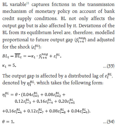

Inflation Expectations

Inflation expectations are determined by the following process: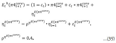

Inflation expectations are a weighted sum of one-quarter lagged year-on-year core inflation, and the model-based rational expectation of year-on-year inflation one quarter ahead. The weights depend on the stock of policy credibility (c_t). c_t can range from 0 (no credibility), in which case expectations are completely backward looking, to 1 (perfect credibility), in which case inflation expectations are perfectly forward looking.

Credibility Stock Building

Credibility, as noted above, is modelled as a stock (c_t) measured between 0 and 1. Credibility changes non-linearly i.e., at lower levels of credibility, monetary policy needs to be sufficiently aggressive to achieve the disinflation. However, as credibility stock increases, the policy reactions can be lower to achieve the same quantum of disinflation.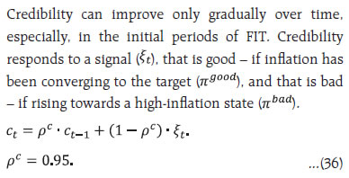

The credibility signal weighs the relative likelihood of inflation converging to the target. It is higher if the current realised inflation is closer to the target. The error under the bad (good) regime is defined as the difference between the realised inflation and the expected inflation under the bad (good) regime.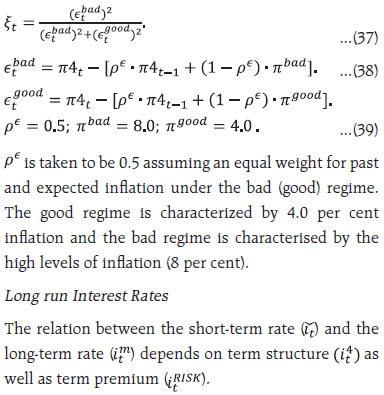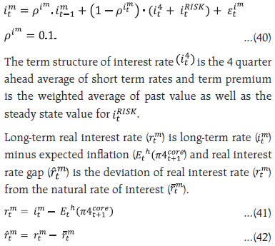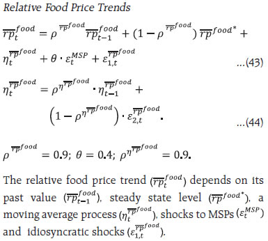

^ The authors are from the Reserve Bank of India.

The views expressed in this article are those of the authors and do not represent the views of the Reserve Bank of India.

¹ This project was carried out under UTKARSH 2022, the medium-term strategy framework of the RBI.

² Data for the period after 2019 were not used as extreme volatility induced by COVID-19 and other developments could affect the average model properties.

³ In the face of capital flows shocks, the exchange rate tends to move significantly away from its long-run equilibrium, causing exchange rate passthrough to inflation and economic dislocation. Hence, central banks care about the exchange rate in addition to inflation. However, paying attention to the exchange rate using monetary policy tools can undermine the credibility in an inflation targeting regime making monetary policy actions costlier (Blanchard et al., 2016, Ghosh et al., 2016).

⁴ All the real trends are system consistent, filtered using Kalman filter. In QPM 2.0, with the incorporation of fuel prices in the aggregate demand equation (equation 1), the world output gap coefficient reflects only the direct effect and has been calibrated accordingly. In QPM 1.0, it reflected the direct effect as well as the indirect impact of crude oil prices.

⁵ Core inflation is defined as inflation excluding food, fuel, petrol and diesel components.

⁶ Inflation expectations formation and an endogenous credibility building process is modelled similar to QPM 1.0 (Appendix and Benes et al., 2016b). π denotes quarter-on-quarter (annualised) inflation, while π4 denotes year-on-year (y-o-y) inflation. The increase in nominal (S_t) and real (Z_t) exchange rates depicts depreciation and vice versa. The relative food price trend is modelled similar to QPM 1.0 (Appendix and Benes et al., 2016b).

⁷ In QPM 1.0, fuel inflation incorporated two types of fuel viz. market and administered. Market fuel inflation was determined by the Indian basket crude oil prices and exchange rate, while the administered component in fuel pricing was largely modelled as an exogenous process (Benes et al., 2016b).

⁸ The coefficient 0.47 corresponds to crude oil prices at around US$80 per barrel.

⁹ Deviation of crude oil price from its long-term trend.

¹¹ The increase in BL variable depicts tightening of bank lending condition and vice versa.