 IST,
IST,
RBI WPS (DEPR): 03/2020: Nowcasting Indian GDP growth using a Dynamic Factor Model
RBI Working Paper Series No. 03 Nowcasting Indian GDP growth using a Dynamic Factor Model @Soumya Bhadury Abstract 1In India, the first official estimate of quarterly GDP is released approximately 7-8 weeks after the end of the reference quarter. To provide an early estimate of current quarter GDP growth, we construct single-index dynamic factors (DFs) using a sequentially expanding list of 6, 9 and 12 high-frequency indicators. These indicators represent various sectors, display high contemporaneous correlation with GDP, and track GDP turning points well. While DF-6 includes domestic economic activity indicators, DF-9 combines indicators of trade and services and DF-12 adds financial indicators in the model. In addition to conventional economic activity indicators, we include a financial block in DF-12 to reflect the growing influence of financial sector on economic activity. DFs are estimated using a dynamic factor model which extracts a common trend underlying the high-frequency indicators. The extracted trend provides a real time assessment of the state of the economy and helps identify sectors contributing to economic fluctuations. Further, GDP nowcast using DFs show considerable gains in both in-sample and out-of-sample accuracy. In particular, our GDP growth nowcast is observed to closely track the recent slowdown in the Indian economy. JEL Classification: C32, C51, C53 Keywords: Nowcast, Economic Cycle, Dynamic Factor Model, Turning Point Analysis, Jagged Edge Data Introduction Real-time assessment of the state of the economy is a pre-requisite for taking appropriate policy measures. The effectiveness of policy-making depends on how well it uses all information available at any given time. Moreover, making use of the current flow of information is an essential ingredient in formulating a forward-looking policy. Today, in a dynamic environment, data driven policy-making is considered both practical and desirable. This is all the more important because of significant lags in official data releases of key macro variables such as GDP. Emerging market economies face serious problems of data lags, gaps and revisions which hamstring optimal policy decisions. A core concern in policy-making is identifying the signs of expansions and contractions in economic activity. At any point, diverse economic indicators may indicate varied trends in activity. Therefore, combining all of these together in an appropriate way to arrive at the underlying (or unobserved) trend has traditionally occupied the attention of both governments and businesses. Traditionally, a lot of work was done in the National Bureau of Economic Research and the Department of Commerce in the US on identifying business cycles using multiple indicators. Often, their analysis relied on prior beliefs and judgement. Later, academic research contributed by making the analysis more formal and mathematically precise (see Stock and Watson, 1989). Presently, this whole exercise displays a mix of both sound conceptual framework, careful inference and judgement. There exists a two-pronged challenge in assessing the underlying state of the economy using high frequency indicators. The first one is the choice of appropriate indicators from a large set of potential indicators. The second challenge is associated with signal extraction from the chosen indicators. This is because individual indicators may reflect short-term idiosyncrasy rather than an underlying general trend. Researchers look at a variety of indicators relating to different aspects of the economy – production, income, sales and employment – together to assess the underlying state of the economy. The consensus trend emanating from all these indicators suggests recessions or expansions (or equivalently slowdowns and accelerations) in economic activity. The dynamic factor tries to address the challenge of signal extraction by identifying the general (or common) trend underlying several activity indicators. To address the first challenge of identifying appropriate indicators, our approach is to weigh indicators based on their information content about the dynamics of GDP. We identify a pool of relevant indicators based on (1) contemporaneous correlations between indicators and GDP; and (2) explanatory power of the indicators around GDP turning points. Based on these two criteria, we choose a set of twelve indicators which includes index of industrial production – consumer goods and core sectors, automobile sales, non-oil non-gold imports, exports, rail freight, air cargo, foreign tourist inflows, government tax receipts, Sensex, Nominal Effective Exchange Rate (NEER) and bank credit. Despite following an independent variable selection approach, our choice of indicators is similar but not the same as Stock and Watson (1989) which used index of industrial production, real personal income, real manufacturing and trade sales, and employee-hours in non-agricultural establishments to construct a Coincident Economic Indicator. One reason for deviating from Stock and Watson (1989) is that in emerging markets such as India, indicators on employment and income are difficult to obtain at high frequency. Therefore, researchers have used suitable proxy variables. The second reason for deviation is the unavailability of data on such indicators for a long period. On the whole, our choice of indicators represents real, external and financial sectors which are used to extract the common underlying trend using a single-index dynamic factor model. We call the estimated indices DF-6, DF-9, and DF-12, based on a sequentially expanding list of 6, 9 and 12 high-frequency indicators, respectively. Given the lags in the release of official GDP, the estimated DFs are used to obtain the current quarter nowcast of GDP. Broadly, the nowcast exercise is an extension of the bridge type regressions that relate GDP to quarterly aggregates of relevant economic indicators. However, we rely on a parsimonious autoregressive model of GDP augmented by monthly DFs. While tracking the actual GDP dynamics closely in the sample, our modelling approach also shows considerable gains in terms of out-of-sample performance. The rest of the paper is organised as follows. Section II provides a comprehensive review of the literature on high-frequency indicators and nowcasting, including cross-country studies as well as the literature specific to India. Section III briefly describes the data used for constructing DFs. Section IV presents the methodology and empirical results on indicator selection, estimation of a dynamic factor model, nowcasting GDP and performance evaluation of our models. We put our concluding remarks in section V. Annexes contain technical details. Nowcasting involves an exercise of predicting the present, the very near future, and the very recent past - that makes it more effective in shorter horizon forecasting (Banbura, Gianonne and Reichlin, 2010). A set of high-frequency indicators is commonly used in GDP nowcasting exercise. Perhaps, the first use of such indicators is found in Burns and Mitchell (1946), which popularized the study of business cycles, and that eventually led to the creation of the composite index of coincident indicators. The methodology has gradually been refined over time and a breakthrough came in the Stock and Watson’s (1989) seminal work on estimating a single-index dynamic factor model (DFM). More recently, Giannone, Reichlin and Small (2008) have pioneered the usage of DFM based on a large number of high-frequency indicators and found that the nowcasts have outperformed standard univariate models like random-walk and autoregressive (AR) models. Generally, a wide variety of high-frequency indicators are actively monitored in gauging the health of an economy. The indicators used are in-sync with the current economic cycle and primarily represent six blocks which include: (a) industry and construction, (b) personal income (or consumption), (c) payroll employment (d) services (e) external sector, and (f) price. These indicators are chosen not merely because of their correlation with GDP, but also because they contain timely information about the target variable. Depending on countries and sample periods, various researchers have also included miscellaneous economic activity indicators (e.g., air cargo, rail freight, and port traffic and uncertainty / volatility indices). Though, most of the financial sector variables (e.g., money supply, currency with public, credit, equity indices and bond indices) are generally classified as lead indicators, some of the studies have incorporated them in GDP nowcasting and documented improvement in their nowcasting performances (Annex Tables I and II report the details). Some researchers have included financial conditions indices (a linear combination of risk spread, asset returns and volatility) to model the risk to output growth one year into the future (IMF, Global financial Stability Report, October 2017). II.1 Cross-country nowcasting models Modern macroeconomic literature emphasizes the role of forward looking assessment of growth and inflation by central banks in policy formulation. Globally, central banks and their monetary policy committees (MPCs) rely on high-frequency economic indicators for an assessment of the current state of the economy. For instance, Bank of England’s MPC uses such a model-based nowcast. Similarly, the Federal Reserve Bank of Atlanta (FRBA)2 and the Federal Reserve Bank of New York (FRBNY)3 publish their own model-based nowcasts in addition to the routine forecast produced in the bank. The European Central Bank4 also consults a DFM-based nowcasting model. Other central banks such as Norges Bank5 uses nowcasting models of GDP for its policy decisions. Outside the ambit of central banks, several country-specific GDP nowcasts have evolved over time. Among the advanced economics (AEs), Kumar (2013) constructed a high-frequency real activity indicator that tracked economic activity in Canada reasonably well. The indicator is obtained as an unobserved common factor capturing the co-movements in real macroeconomic variables. Similarly, Chikamatsu et al. (2018) produced nowcasts of quarterly GDP estimates for Japan by adopting a bridge equation approach. The bridge equation links the low-frequency target variable with the high-frequency indicators. Annex Table I provides an exhaustive list of variables used by the authors. While DFM based nowcasting models have been adopted for a long time across advanced economies, emerging market economies (EMEs) have started exploring the usefulness of such models only recently. For instance, Luciani et al. (2015) used high frequency indicators (e.g. cement, PMI-manufacturing, consumer confidence, auto sales, etc.) for Indonesia in estimating a dynamic factor and then used the same to nowcast GDP growth in an autoregressive, bridge-equation framework. Caruso (2015) used the Maximum Likelihood estimation in an expectation-maximization (EM) algorithm for constructing an economic activity index for Mexico. The EM algorithm is useful in analyzing non-synchronous data releases that are often observed in EMEs. II.2 Nowcasting Indian GDP Among the emerging markets, India has a reasonably long history of research in tracking and nowcasting GDP. Early works in this domain include Dua and Banerji (2001), and Technical Advisory Group constituted by the Reserve Bank of India (2007). Dua and Banerji (1999) published an index of monthly coincident indicators to help ascertain the timing of recession and expansion of economic activity based on a set of objective indicators that are synchronous with cyclical fluctuations in growth. Some of the indicators (e.g. monthly unemployment numbers published in the Monthly Abstract of Statistics) are not published anymore. However, we report an update of this monthly index, using available data and proxy variables, in the Annex Note I. Along similar lines, Reserve Bank of India (2007) published a set of indicators including Composite Index of Leading Indicators (CILI) and Composite Index of Coincidental Indicators (CICI) based on a detailed empirical exercise using growth cycle and growth rate cycle methodologies. CILI and CICI were mainly based on principal component analysis (PCA) with sample data spanning from April 1990 to March 2006. Recent academic research, such as Dalhaus et al. (2017) and Bragoli and Fosten (2017) adopted a standard dynamic factor model (DFM) framework for GDP growth nowcasting. Both these studies attempted to extract monthly unobserved common factor from a set of monthly indicators. Following factor extraction, monthly projection of GDP growth is estimated based on the dynamics of the common factor. The indicators used in these studies are summarized in Annex Table II. Dua and Sharma (2016) used a univariate Markov regime switching model to characterize growth cycle phenomena and distinct economic regimes for India and compared them with the US, UK, Germany and Japan. In addition to academia and central banks, market research organizations, think-tanks, and professional economists have estimated and published indices based on high-frequency indicators and used them to nowcast India’s GDP. For instance, Rabobank6 uses different models to nowcast India’s GDP growth that include Bayesian VAR (BVAR), OLS and a combined model, which help in deriving the underlying contribution of high-frequency indicators in GDP growth forecasts. Besides economic indicators, Rabobank also includes financial indicators such as monetary base (M0), volatility index (VIX), BSE-500 index and Sensex. National Institute of Public Finance and Policy (NIPFP) estimated common factors using PCA and then used three different variants of bridge equation models. The NIPFP working paper (Bhattacharya et al., 2010) used variables from several sectors of the economy that included industrial production, construction, services and financial sectors and documented that the empirical strategy outperformed the benchmark AR models. An NCAER working paper (Bhadury et al., 2018) presented a new framework to nowcast India’s GVA using information of mixed da, 2018ta frequencies and adding evening-hour luminosity information to capture economic activity of informal sectors in India. In India, professional economists (economists with banks, brokerage houses and think tanks) also regularly nowcast GDP using proprietary models. Some of the GDP nowcasts by these economists are also published by the Bloomberg7, however, their exact nowcasting methodologies are not in the public domain. Bloomberg also publishes its Monthly GDP tracker to provide an advance estimate of the current quarter economic activity in India. The Monthly GDP tracker is constructed by applying weights to the monthly activity indicators, such as agricultural trade balance, real currency demand, industrial production, etc. (details in Annex Note I) and the weight assigned to each monthly indicator is the inverse of the standard deviation of the respective indicator. To summarize, the use of economic activity indicators in GDP nowcast has a long history in advanced economies and still being actively used in monetary policy-making by the central banks. Though there have been debates relating to inclusion of high frequency variables, their lead, lag or cotemporaneous characteristics, nowcast exercise has moved on by including new blocks of variables with an objective to improve nowcast performance. The application of high-frequency variables in GDP nowcasting is relatively new in emerging market economies and have been challenged by small sample size, non-synchronous data releases and varying data lags. However, considering its importance in policymaking, economists have been striving with new empirical strategies to bridge this gap and use such indicators as an active policy tool. Our attempt here is to construct an index for the Indian economy that tracks business cycle reasonably well. The first best is always the quarterly estimates of GDP at constant prices which is published by the Central Statistical Office (CSO)8 with a lag of two months. Given the delay in data release, we use dynamic factors in providing the current-quarter nowcast of GDP, our target variable. The indicators used in the construction of DF-6, DF-9 and DF-12 represent all relevant sectors of the Indian economy. Data published on a monthly frequency is exploited to construct the DFs and are sourced from the CEIC database.9 The high-frequency monthly series associated with industry and construction block is IIP-core industries. Personal income and consumption block is represented by indicators such as IIP-consumer goods and auto sales. Exports, non-oil and non-gold imports and foreign tourist arrivals represent the external sector block. Rail freight, air cargo and government revenue receipts represent services and miscellaneous economic activity, respectively. The above indicators are included in DF-6 and DF-9. In addition, we develop a DF-12 that adds a credit and finance block by including non-food credit, NEER and Sensex. Though in the literature, equity index and credit, in some instances, have been classified as lead indicators, we explain the rationale for including these variables in the DF-12 in the discussion on variable selection. At this juncture, it might be important to mention that the GDP series has been revised and rebased in India from time to time. For instance, on November 28, 2018 the Ministry of Statistics and Programme Implementation released the annual back series of data beginning 2004-05 (at 2011-12 prices). As per the new series, GDP growth has been revised downward during 2004-05 to 2011-12 compared to the earlier 2004-05 series. However, the Ministry has not separately released the back series of the quarterly data. Therefore, we rebase the older 2004-05 and 1999-2000 series to match the 2011-12 quarterly data.10 IV. Methodology and Empirical Results The empirical exercise entails variable selection, standardization, smoothing and appropriately combining these transformed variables into an index. This index is then used for GDP nowcasting. We approach the above empirical exercise in four sequential stages in the following manner. IV.1 Variable Selection Variable selection is perhaps the most crucial part of the exercise. Our aim is to include indicators that capture the pronounced and persistent movements in economic activity. We look at the availability of high frequency data for over sufficiently long period and the literature that is particularly relevant for India e.g. Dua and Banerji (2000), and Reserve Bank of India (2007). We begin with an extensive survey of the international literature relating to high-frequency indicators that are used in producing real time assessment of GDP growth (see Annex Tables I and II). Based on the review of literature, we shortlist 28 high-frequency indicators for the Indian economy. These indicators represent all major sectors in the economy, such as industry and construction, personal income and consumption, employment, services, external sector, prices, credit and finance, and miscellaneous economic activity. The summary Table 1(a) below reports the indicators and the sectors that they represent in the economy. We attempt to nowcast GDP using available high frequency indicators for the reference quarter. In doing so, we focus on those high-frequency indicators that will capture the GDP dynamics but would avoid overfitting. Therefore, while we start with an exhaustive list of high-frequency indicators including those used by National Statistical Office (NSO), we finally select 6, 9 and 12 indicators representing all major sectors in the economy. Based on the nowcasting literature, the selected indicators represent production, income, consumption and sales activities. Thus, they represent a mix of both expenditure and production side. The summary Table 1(b) below reports some of the key indicators used by NSO to provide the first advance estimates of quarterly GVA. Our list of indicators includes many of those used by NSO for GVA compilation. Additionally, we take into consideration indicators that proxy income/consumption, employment, prices, and external sector. Our second round of indicator screening is based on the dynamic correlation between indicators and the target variable i.e., GDP. In addition to examining the correlation of indicators with the target variable over the full sample, we also pay special attention to dynamics around turning points in GDP. In emerging markets including India, GDP dynamics is seen to be more volatile displaying significant accelerations and decelerations in growth in quick succession. Therefore, a desirable feature of indicator selection would be to capture such dynamics. To achieve this, we use a forward step-wise and Lasso selection procedure to identify the set of 12 high-frequency indicators that are relevant around turning points in India’s GDP. Dynamic Correlation We look at the correlation of Q-o-Q seasonally adjusted annualized growth of the variables with our target variable, GDP. The dynamic correlation analysis is carried out over 2003:Q1 to 2019:Q1 with around 65 observations at different leads and lags of GDP. We have identified variables as Cotemporaneous (‘C’), Leading (‘L+’) and Lagging (‘L-’) indicators depending on their contemporaneous, future and past correlations, respectively with GDP. These correlation coefficients and their statistical significance are presented in the Annex Table III. Among the economic indicators, the highest contemporaneous correlation with GDP is observed for Sensex, IIP-consumer goods and air cargo. Finally, a few indicators such as IIP-core, commercial automobile sales and forex reserves display both cotemporaneous and leading properties in terms of their correlations with contemporaneous and future GDP. The summary Table 1(c) below reports the dynamic correlation coefficients for the shortlisted high-frequency indicators. Next, we use the forward step-wise selection, followed by the Lasso procedure to identify indicators that are relevant around turning points in GDP. The notion of using indicators to discern business cycle peaks and troughs is not new in the growth literature. Our aim is similar in spirit to that of Moore (1950) i.e., identify turning points in India’s business cycle using high-frequency indicators. Such indicators can provide a sense of recession risks, and enable policymakers and business-decision makers to have a better-informed analysis of the economic situation. OECD has a methodology to identify turning points using Composite Leading Indicators (CLI). CLI is periodically measured by OECD for 33 member countries and 6 non-member countries including Brazil, China, India, Indonesia, Russia and South Africa11. Unlike several advanced and emerging market economies, Indian economy has not experienced economic contractions or recessions in the last few decades. Instead, it is characterised by accelerations and slowdowns in growth rate around a (time-varying) trend level of GDP growth (see Acharya et al., 2020). Accordingly, we identify turning points in India, keeping in mind the “growth rate cycle” instead of “growth cycle”. Our approach of capturing the “growth rate cycle” helps us identify more turning points for India compared to the OCED approach because it is based on identifying short-duration cycles to capture volatility in GDP instead of relying only on long-duration cycles. Chart 1 below plots the real GDP growth and its turning points for India. 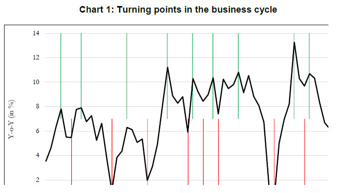 Forward Step-wise Selection The forward step-wise selection procedure is a computationally efficient alternative which sequentially add candidate variables to assess their predictive power around the turning points in GDP. In particular, at each step the variable that gives the highest incremental improvement (to the fit) is included in the model. The summary Table 1(c) below provides a relative ranking of the variables in terms of their relevance around turning points. In terms of relative ranking, IIP-Consumer goods, auto sales and NEER have highest relevance around the turning points in GDP. Lasso  Lasso yields a sparse model, which involves a subset of the variables that make model interpretation easier. Based on the Lasso criterion, a list of indicators that are found to be relevant around turning points in the GDP growth cycles is reported in the summary Table 1(c). Lasso technique suggests that indicators such as IIP-consumer goods, auto sales, NEER, IIP-core, rail freight, Sensex and exports are relevant for India’s GDP turning points. Interestingly, the forward step-wise selection method assigns the highest rank to the same set of indicators, thereby confirming the relevance of such indicators around turning points.
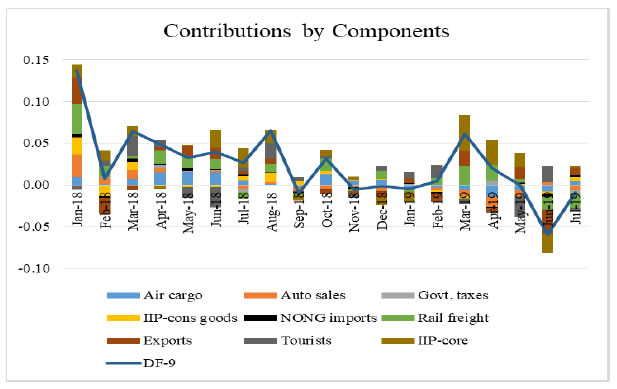
To summarize, our main objective is to construct an economic activity index for India based on high-frequency indicators that co-move strongly with the target variable. Our first and second rounds of screening are based on the review of literature and dynamic correlations between high-frequency indicators and GDP, respectively. Further, to refine relevant indicators around turning points, we look at the forward step-wise selection and Lasso criteria. In the next section, we construct a battery of economic activity indices that include a DF-6 model covering exclusively domestic economic activity indicators, a DF-9 model incorporating trade and services sector, and finally a DF-12 which incorporates financial variables. Furthermore, we equally consider experts’ views, literature and judgement in identifying and grouping variables. IV. 2 Dynamic Factor Model After selecting the relevant variables to be incorporated in our model, we proceed to estimate a single factor representing the common trend underlying these variables. The single factor is obtained by estimating a dynamic factor model (DFM), a procedure widely popular in the recent literature. For analytical clarity, we sequentially estimate 6-indicators, 9-indicators and 12-indicators DFMs. Our dynamic factor model contains the following set of equations representing a state-space form.  We estimate the DFM using a multivariate autoregressive state-space model12. The time-series of economic indicators (y) is modelled as a linear combination of the hidden trend (x) and factor loadings (Z) plus some offset ‘a’. For example, the DF-6 model consists of IIP-consumer goods, non-oil and non-gold imports, domestic auto sales, rail freight, air cargo and government receipts represented by six observed time series. The model extracts the common underlying trend in the observed time-series as a single-index dynamic factor. The MARSS specification consists of two stochastic components: an unobservable common component, xt and an idiosyncratic component vt. Both of these components are modelled as autoregressive stochastic processes. xt is an estimate of DFs and Z represents the loadings of the economic indicators on the common component. The identifying assumption in the above model is that the co-movements in the time series indicators arise from the single source xt, i.e. xt enters each indicators with different loadings, Zi, i=1…. ,6. This is ensured from our assumption that vit and xt are mutually uncorrelated at all leads and lags for all the 6 observed economic indicators. The same model is estimated further by including three additional variables (DF-9) and six additional variables (DF-12). It is noted that all these three track actual GDP turning points quite closely. An important issue is related to the choice of number of indicators in generating dynamic factors. While it makes sense to derive a dynamic factor based on a large set of economic indicators, typically 100 or more, however, from a policy point of view it is more meaningful to generate an economic activity index based on a set of shortlisted indicators. We have multiple rounds of screening procedure to weed out indicators that are either not significantly correlated with GDP series or not significantly relevant around turning points in GDP. A dynamic factor generated out of relevant indicators can accurately help us gauge the contribution made by activity indicators, especially identify indicators that are driving or dragging the dynamics in the common factor. Next, we focus on the dynamics of DF-6 in the recent quarters. Chart 2 represents both year-on-year (Y-o-Y) and month-on-month (M-o-M) variation in DF-6. To iron out the monthly fluctuations, we present three-month moving average of both the series. The M-o-M series indicates monthly momentum in economic activity while the Y-o-Y series captures the yearly dynamics. The M-o-M series suggests a sharp deceleration coinciding with the period of demonetization, and also a sharp recovery quickly thereafter. Subsequently, since early 2018, the monthly momentum suggests a gradual moderation in economic activity. The Y-o-Y series, like the monthly series, captures the demonetization downturn and the subsequent recovery, which peaked in December 2017, helped by the low base of the previous year. The Y-o-Y series also suggests economic deceleration as indicated by the M-o-M series since early 2018 (Chart 2). 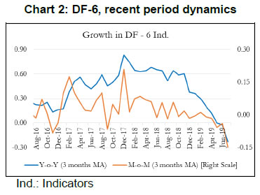 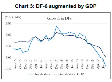 Some authors include GDP along with other high frequency indicators of activity to construct a coincident indicator (Dua et al. 1999). Following this, we also include GDP in DF-6 which is represented in Chart 3.13 It is noted that the dynamics of DF-6 doesn’t change considerably with/ without GDP and both indicate a downturn in economic activity in 2018-19. Chart 4 plots the contribution14 of each of the indicators included in the model to explain the variation in M-o-M (3 months MA) DF-6. We also report the contribution of each indicator in Table 2. It is evident that recent deceleration has been broad based. Both consumption indicators – auto sales and IIP-consumer goods, and investment indicators – rail freight and air cargo have contributed significantly in the recent deceleration. 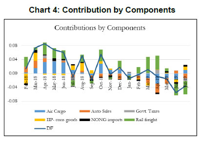 As indicated earlier, we expand our indicator list to include IIP-core, foreign tourist flows and exports. These additional variables represent investment and services activities. Chart 5 plots the recent dynamics of DF-9, which is in line with DF-6. It is noted that while broadly tracking economic activity well, DF-6 and DF-9 still miss some of the turning points, for example the quarter ending June 2017, which was impacted by Goods and Services Tax led disruption, and the extent of the recent slowdown (Chart 8). To address this problem in DF-6 and DF-9, we augment the model by including a financial block to improve the tracking of GDP growth, our target variable. While some of the financial variables might display leading properties and therefore deviate from the core principles of tracking contemporaneous economic activity, we still included Sensex, bank credit and NEER which are likely to better capture turning points (MSM No.10).15 DF-12 points towards some recovery in economic activities, contrary to DF-6 and DF-9, in the recent times (Chart 6). This is on account of a sharp improvement observed in all financial indicators – bank credit, Sensex and NEER – in the recent period painting a somewhat optimistic picture of economic activity. 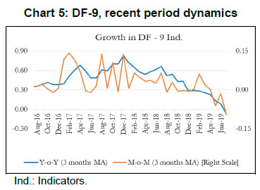 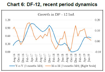 IV. 3. Nowcasting India’s GDP Growth Taking a cue from the literature, we use the estimated DFs to nowcast current quarter GDP growth well before (at least 8 weeks in advance) the official release. For this purpose, we estimate a parsimonious AR model of GDP growth augmented by DFs (Y-o-Y). The model estimates are presented in Table 3. The nowcasts based on 6, 9 and 12 indicator models along with actual GDP growth are plotted in Chart 7. It is observed that the GDP nowcasts track the actual GDP growth reasonably well over the estimation sample. It is also observed that the nowcasts were able to track the recent slowdown particularly well (Chart 8). 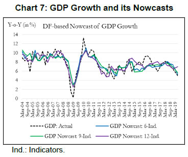 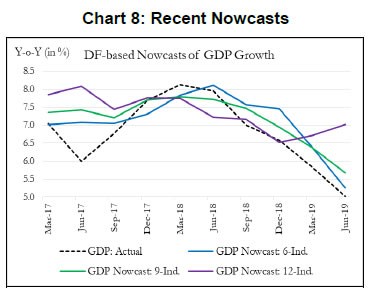 IV.4. Model Performance The next step in model building pertains to the evaluation of model performance. We estimate a parsimonious AR model of GDP growth augmented by DFs (Y-o-Y). Alternatively, we could have used multiple time series indicators in a bridge equation framework to nowcast current quarter GDP growth. We prefer the former keeping in view the problem of overfitting. In time-series, we encounter the overfitting problem when the model starts to learn inherent idiosyncrasies in the training data to the extent that the performance of the model gets severely impacted on new dataset. This is only possible when the random fluctuation in the training sample gets picked up as a consistent pattern by the model and, thereby, hinders the model’s ability to produce credible forecast/nowcast. One way to prevent the problem is to generate dynamic factors that can capture the common trend underlying several economic activity indicators. In other words, instead of fitting multiple time series indicators in a bridge equation framework to nowcast current quarter GDP growth, we prefer estimating a parsimonious AR model of GDP growth augmented by DFs. Keeping in mind structural change (or crisis) in the economy, one should rely on the robustness of the model, and not just on optimization based on backfitting which works only for the past and is often suboptimal for the future. Accordingly, we examine the out-of-sample performance of the nowcasting models during 2017Q1-2019Q1. It is observed that the out-of-sample performance, measured in terms of root mean squared error (RMSE), is better for the DF-6 model compared to the DF-9 and DF-12 models (Chart 9 and Table 4). We further examine forecast accuracy gains obtained from DF based growth nowcast estimates that have incremental information in the form of jagged edge data embedded in them. The high-frequency economic activity data releases in India are non-synchronous in nature. For example, monthly production of coal and crude oil is typically released on the last working day of the month, monthly production of commercial vehicles is released during the middle of a month, and railway freight traffic (of major commodities) is released during the first 10 days of every month. Also, there are varying lags in data releases. Together, this results in jagged-edge data. The out-of-sample performance suggests that DF-based nowcasts obtained from jagged-edge data structure perform marginally better than nowcast estimates obtained from data set without rough edges. The jagged-edge DF estimates consistently record a lower RMSE for 6, 9 and 12-indicator models compared to those without jagged edges. Next, we apply mixed data sampling (MIDAS) regression to exploit the rich information contained in our monthly DFs to nowcast quarterly GDP and improve out-of-sample performance. We compare the models that adopt OLS method with those that use MIDAS method, which are specially equipped to handle mixed frequency data (details in Annex Note III). In general, the baseline DF-6 model performs better out-of-sample compared to DF-9 and DF-12 models. However, we do not observe much of a forecast accuracy gains from applying MIDAS over OLS regression for DF-6, DF-9 and DF-12. 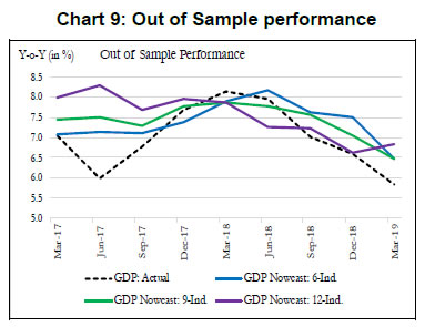
To do a comparative analysis of GDP nowcast performance across different models, we report the out-of-sample performance of 6-indicator, 9-indicator and 12- indicator models. Table 3 reports the out-of-sample root mean squared error (RMSE) over the recent nine quarters i.e., 2017Q1-2019Q1. We compare the models that utilize dataset with jagged edges and use MIDAS with those that do not, for the 6- indicator, 9-indicator and 12-indicator models. The 6-indicator model using the jagged edge dataset records the lowest out-of-sample RMSE. Broadly, the analysis from using the jagged edge dataset seems to suggest that by exploiting the incremental information that is available from the actual flow of data releases, we are able to improve model performance. We evaluate the performance of our model against that of the professional forecasters and market analysts. In this context, as mentioned in Section II, professional forecasters use their proprietary models, and they share their projections with Bloomberg. We plot the mean of such projections along with DF based nowcasts (Chart 10). In terms of forecast performance, DF-6 and DF-9 display accuracies comparable to that of the professional forecasters. In addition, DF based model is able to track turning points timely because it exploits the current flow of information available in high frequency indicators instead of only relying on a backward looking information set. 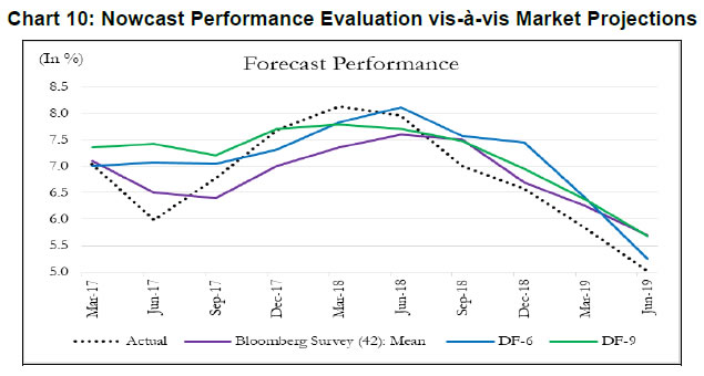 Finally, as a test of robustness, we compare the dynamics of DFs with an alternative and unconventional measure of economic activity captured in the nightlight data (luminosity index).16 Notwithstanding the seasonality (September–October spike), limited availability (up to 2017) and aggregation problems (national average), luminosity index is expected to capture economic activities well, particularly in economies with dominant informal sectors. It is reassuring to note that Y-o-Y dynamics of DF-6 corresponds well with the nightlight data, which is provided by an independent source and is being extensively used of late (Chart 11). 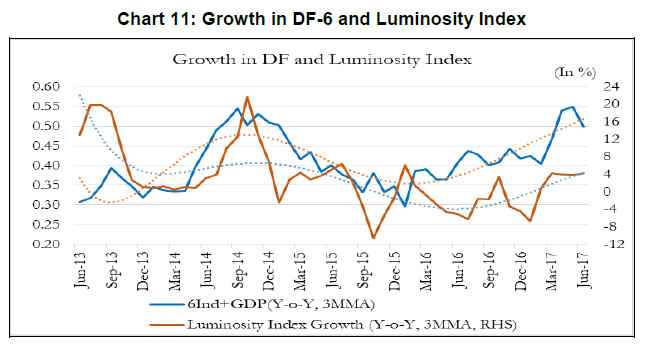 A core concern in policy-making is identifying the signs of expansions and contractions in economic activity. At any point in time, diverse economic activity indicators may indicate mixed trends. Therefore, combining all of these together in an appropriate way to arrive at the underlying (or unobserved) trend has traditionally occupied the attention of both governments and businesses. Our aim has been to contribute to the existing literature by combining high frequency indicators, which are useful proxies of economic activity, to nowcast GDP growth of India. To provide an early estimate of the current quarter GDP growth, we construct single-index dynamic factors using 6, 9 and 12 high-frequency indicators. These indicators represent various sectors, display high contemporaneous correlation with GDP, and co-move in line with the GDP turning points. While DF-6 includes domestic economic activity indicators, DF-9 combines indicators of trade and services and DF-12 adds financial indicators in the model. In addition to conventional economic activity indicators, we include a financial block in DF-12 to reflect the growing influence of financial sector on economic activity. DFs are estimated using a dynamic factor model which extracts a common trend underlying the high-frequency indicators. The extracted trend provides a real time assessment of the state of the economy and helps identify sectors contributing to economic fluctuations. Further, GDP nowcast using dynamic factors show considerable gains in in-sample and out-of-sample accuracy. In particular, DF based nowcast is observed to closely track the recent slowdown in the Indian economy. @Soumya Bhadury is Manager-Research in the Strategic Research Unit (SRU), Reserve Bank of India (RBI) (soumyasbhadury@rbi.org.in). Saurabh Ghosh (saurabhghosh@rbi.org.in) and Pankaj Kumar (pankajk@rbi.org.in) are Directors in SRU, RBI. 1 The views and opinions expressed in this paper are those of the authors and do not necessarily represent those of RBI. Authors would like to thank Prof. Pami Dua, Dr. Jay Surti, and seminar participants in DEPR Study Circle and CAFRAL for their valuable comments and suggestions. 2 GDPNow forecasting model by FRBA does a "nowcast" of the official estimate prior to its release by estimating GDP growth using a methodology similar to the one used by the U.S. Bureau of Economic Analysis. 3 The FRBNY nowcast model produces forecasts of GDP growth for all variables taking into account their dynamic interactions. 4 The European Central Bank models the monthly data as a parametric dynamic factor model cast in a state-space representation against the quarterly GDP. 5 Norges Bank analyzes unstructured textual information of a business newspaper to decompose daily news topics and nowcast quarterly GDP growth for policy rate decisions. 6 Rabobank combines predictions from Bayesian Vector Autoregressive (BVAR) model and an Ordinary Least Square (OLS) model for GDP forecasts. Link: https://economics.rabobank.com/publications/2019/february/nowcasting-the-indian-economy/ 7 Bloomberg tracks real time GDP data using a weighted methodology to nowcast GDP from high frequency volume based economic indicators. 8 The Ministry of Statistics and Programme Implementation has decided to merge the CSO and National Sample Survey Office (NSSO) into National Statistical Office (NSO). 9 CEIC is a data aggregator that collects data from different ministries, government documents and other data originators. 10 As a robustness exercise, we also use the downwardly revised Y-o-Y growth of the new back series. This, however, does not change our estimates significantly. 11 OECD uses the turning point detection algorithm, which is a simplified version of the original Bry and Boschan (B&B) routine. B&B routine parses local minima and maxima in the cycle series and applies the censor rules to guarantee alternating peaks and troughs. OECD’s CLI based approach has identified 10 such turning points for the Indian economy with +1 set for a peak and -1 set for a trough. The reference chronology of the turning points are as follows: trough in October-1997, peak in December-1999, trough in January-2003, peak in September-2007, trough in March-2009, peak in December-2010, trough in July-2013, peak in March-2016, trough in July-2017, and peak in May-2018. 12 The model is estimated using the MARSS package in R. 13 In our sample, quarterly GDP is available until June 2019. The jagged edge methodology is used to handle the missing observations of GDP for recent months. 14 Contribution of a component = M-o-M growth of component*Regression coeff. of M-o-M growth in component on M-o-M growth of DF. 15 /en/web/rbi/-/working-capital-constraints-and-exports-evidence-from-the-gst-rollout 16 Infrared Imaging Radiometer Suite (VIIRS) of National Aeronautics and Space Administration (NASA) and National Oceanic and Atmospheric Administration (NOAA), USA. VIIRS data has a wider radiometric detection range than former generation of similar satellites, which solves the issue of over-saturation at bright core centres (Elvidge et al. 2013). However, the publicly available VIIRS data still requires processing before use, as some temporary lights and background noise remain. We follow the procedure discussed in Beyer et al. (2018) and remove all observations from areas categorized as background noise mask. After outlier removal, these areas are identified by clustering the remaining observations based on their intensity. References Acharya, V., Bhadury, S., & Surti, J. (2020). Financial Vulnerabilities and Risk to Growth in India. Forthcoming. Bańbura, M., & Modugno, M. (2014). Maximum Likelihood Estimation of Factor Models on Datasets with Arbitrary Pattern of Missing Data. Journal of Applied Econometrics, 29(1), 133-160. Bańbura, M., Giannone, D., & Reichlin, L. (2010). Large Bayesian Vector Auto Regressions. Journal of Applied Econometrics, 25(1), 71-92. doi: 10.1002/jae.1137 Bhadury, S., Pohit, S., & Beyer, R. (2018). A New Approach to Nowcasting Indian Gross Value Added. NCAER Working Paper No.115, National Council of Applied Economic Research. Bhattacharya, R., Pandey, R., & Veronese, G. (2011). Tracking India Growth in Real Time. National Institute of Public Finance and Policy, Working Papers 11/90. Bok, B., Caratelli, D., Giannone, D., Sbordone, A., & Tambalotti, A. (2018). Macroeconomic Nowcasting and Forecasting with Big Data. Annual Review of Economics, 10(1), 615-643. doi: 10.1146/annurev-economics-080217-053214 Bragoli, D., & Fosten, J. (2018). Nowcasting Indian GDP. Oxford Bulletin of Economics and Statistics, 80(2), 259-282. doi: 10.1111/obes.12219 Burns, A., & Mitchell, W. (1946). The Basic Measures of Cyclical Behavior. In Measuring Business Cycles (pp. 115-202). National Bureau of Economic Research Book Series Studies in Business Cycles. Caruso, A. (2015). Nowcasting Mexican GDP. European Center For Advanced Research In Economics and Statistics Working Paper No.40. Chikamatsu, K., Hirakata, N., Kido, Y., & Otaka, K. (2018). Nowcasting Japanese GDPs. Bank of Japan Working Paper Series, 18-E-18. Dahlhaus, T., Guénette, J., & Vasishtha, G. (2017). Nowcasting BRIC+M in real time. International Journal of Forecasting, 33(4), 915-935. doi: 10.1016/j.ijforecast.2017.05.002 Dua, P., & Banerji, A. (1999). An Index of Coincident Economic Indicators for the Indian Economy. Journal of Quantitative Economics, 15, 177-201. Dua, P., & Banerji, A. (2001). An Indicator Approach to Business and Growth Rate Cycles: The Case of India. Indian Economic Review, 36(1), 55-78. Dua, P., & Sharma, V. (2016). A Comparison of Economic Indicator Analysis and Markov Switching Methods Concerning the Cycle Phase Dynamics. Journal of Business Cycle Measurement and Analysis, OECD, 2015(2), 1-27. doi: 10.1787/jbcma-2015-5jm22pfhmhlp Ghysels, E., Santa-Clara, P., & Valkanov, R. (2004). The Midas Touch: Mixed Data Sampling Regression Models. CIRANO Working Papers, CIRANO. https://EconPapers.repec.org/RePEc:cir:cirwor:2004s-20 Giannone, D., Reichlin, L., & Small, D. (2008). Nowcasting: The Real-Time Informational Content of Macroeconomic Data. Journal of Monetary Economics, 55(4), 665-676. doi: 10.1016/j.jmoneco.2008.05.010 Kumar, G. (2013). High-Frequency Real Economic Activity Indicator for Canada. Bank of Canada Working Paper, 2013(42). Luciani, M., Pundit, M., Ramayandi, A., & Veronese, G. (2018). Nowcasting Indonesia. Empirical Economics, 55(2), 597-619. Moore, G. (1950). Statistical Indicators of Cyclical Revivals and Recessions. New York: National Bureau of Economic Research. Reserve Bank of India. (2007). Report of the Technical Advisory Group on Development of Leading Economic Indicators for Indian Economy. Stock, J., & Watson, M. (1989). New Indexes of Coincident and Leading Economic Indicators. Macroeconomics Annual, National Bureau of Economic Research, 4, 351-409. 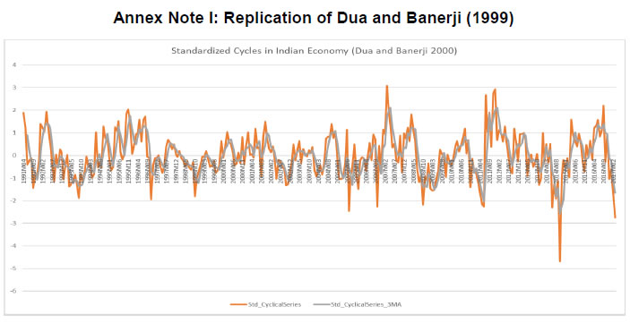 Step involved in replication and updating 1. All data monthly, and seasonally (Census X-11) adjusted
2. Output: Two different measures of CEI which correspond to the following two different variables for output:
3. Index of Industrial Production: Monthly data available
4. Income: Annual wage data from the ASI are interpolated into monthly data using a monthly adjustment factor.
Employment: Monthly seasonally adjusted unemployment numbers from the Monthly Abstract of Statistics (MAS)
5. Trade: In this paper, trade is all domestic. Industrial production of consumer goods at constant prices and seasonally adjusted. 6. Data on actual production levels are not available. We therefore use monthly consumer goods IIP – after necessary splicing to get monthly series at the 1980-81 base.
 The explanatory variables can also have frequencies different from each other. The basic equation for MIDAS is similar to that of distributed lag models, exhibiting a dynamic relationship between the dependent and independent variables. However, there are still significant differences between the two methods. The basic equation for MIDAS is (Ghysels et al. 2004): 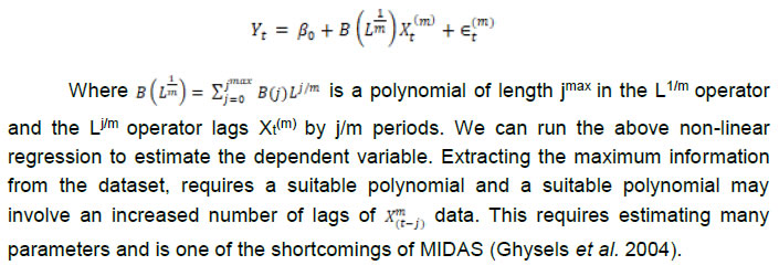 | ||||||||||||||||||||||||||||||||||||||||||||||||||||||||||||||||||||||||||||||||||||||||||||||||||||||||||||||||||||||||||||||||||||||||||||||||||||||||||||||||||||||||||||||||||||||||||||||
கடைசியாக புதுப்பிக்கப்பட்ட பக்கம்:


