 IST,
IST,


RBI WPS (DEPR): 10/2022: Monetary Policy Transmission in India under the Base Rate and MCLR Regimes: A Comparative Study
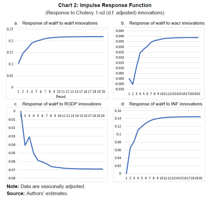
| RBI Working Paper Series No. 10 Monetary Policy Transmission in India under the Base Rate and MCLR Regimes: A Comparative Study Sadhan Kumar Chattopadhyay and Arghya Kusum Mitra@ Abstract *The paper estimates the degree of pass-through of monetary policy to bank lending rates under both the base rate and the marginal cost of funds based lending rate (MCLR) regimes using dynamic panel data regression. Using nine different models for nine individual bank-specific variables, the study estimates that a 100 basis point increase in the policy rate leads to an increase in the weighted average lending rate on fresh rupee loans sanctioned by banks over the long run by 26-47 basis point - depending on the model specification - during the MCLR regime as against 11-19 basis point during the base rate regime. Hence, irrespective of the model chosen, transmission is higher during the MCLR regime than base rate regime. The alignment of liquidity management with the monetary policy stance, introduction of the flexible inflation targeting (FIT) framework and the deceleration in economic activity reducing credit demand could be contributory factors for better transmission during the MCLR regime. JEL classification: E44, E51, E52, G21 Key Words: Monetary Policy, monetary transmission, Generalized Method of Moments (GMM), Arellano-Bond model. Introduction The effectiveness of the monetary policy transmission is built on the idea of how much and how fast monetary policy can influence its ultimate goals, viz., price stability and growth. In India, the banking system being the pre-dominant sector for financial intermediation, it is imperative that monetary policy signals pass through the banking system without any ‘leakage’ and in quick time. Effective transmission requires fulfillment of various pre-conditions. A crucial pre-condition is transparency in the process of pricing of loans by banks, not only for customer protection but also for better assessment of transmission by the monetary authority. In India, simultaneously with interest rates deregulation in October 1994, the banking regulator has been stipulating the adoption of a specific benchmark for pricing of loans by banks. Benchmarks can be either internal to the banks like the cost of funds or lending rates charged to the best customers, or it can be external to the banking system, e.g., market determined T-bill rate. Since deregulation of lending rates was one of the first steps towards financial sector liberalisation which had begun a couple of years ago, no suitable external benchmark was available for the pricing of loans. Accordingly, RBI mandated an internal benchmark – prime lending rate (PLR) - in October 1994.1 In April 2003, the RBI supplanted PLR with the benchmark PLR (BPLR), which was followed by the base rate in July 2010 and MCLR in April 2016. None of these benchmarks met the expectations. Effective October 2019, RBI mandated an external benchmark system for retail and micro & small enterprises (MSE) sectors, which was expanded to include medium enterprises, effective April 2020. Against this backdrop, this study examines the nature of pass-through to lending interest rates in India under three different internal benchmark regimes, viz., BPLR, base rate and MCLR during the period April 2004-July 2019. For econometric analysis, however, our study covers the period Q4:2012-13 to Q2:2018-19, where we study the interest rate channel of monetary transmission in India during the base rate and the MCLR regimes using the quarterly bank-level data of all domestic banks.2 The beginning of the time period of our study is keeping in view the availability of data on the main variable under study. To our knowledge, it is probably the first study of its kind where transmission during two different interest rate benchmark regimes has been compared. Section II surveys the literature on the related fields which are relevant to our study. Section III discusses the stylised facts covering the three internal benchmark regimes. Section IV deals with the data and methodology for econometric analysis adopted in the study. Section V presents the empirical findings. Concluding remarks are provided in Section VI. Literature on monetary policy transmission and its channels is nearly a century old, starting, perhaps with Keynes (1936). Some of the key contributors to the literature over the decades include Friedman and Schwartz (1963), Ando and Modigliani (1963), Tobin (1969), Taylor (1995), Obstfeld and Rogoff (1995), Meltzer (1995), Bernanke and Gertler (1995) and Edward and Mishkin (1995). More recently, Mohanty and Turner (2008), Mukherjee and Bhattacharya (2011), Mishra et al. (2010), and Trichet (2011) examined the efficacy of various channels of the monetary transmission mechanism for both developed and emerging market economies. During the last 20 years, there have been a plethora of studies on monetary transmission in India. These studies include, inter alia, Singh and Kaliranjan (2007), Bhattacharya, Patnaik and Shah (2010), Aleem (2010), Pandit and Vashisht (2011), Sengupta (2014) and Das (2015). There have been several studies on monetary transmission by researchers from the Reserve Bank of India. Mention may be made of Singh (2011), Khundrakpam (2011), Khundrakpam and Jain (2012), Patra and Kapur (2012), Mohanty (2012), Kapur and Behera (2012), Bhoi et al. (2017), etc. These studies have examined the monetary transmission mechanism by taking the Indian data. Most of the initial studies in the international literature have employed aggregate time-series data to examine monetary policy transmission in their analyses. Over the last three decades or so, studies have often employed individual bank-level data to capture the effect of bank-specific characteristics to examine the effectiveness of various channels of monetary transmission mechanism. In this respect, Gambacorta (2008), Were and Wambua (2014), Altavilla et al. (2016), Yang et al. (2016), Holton et al. (2018), Gambacorta and Shin (2018), Abuka et al. (2019), Sapriza, et al. (2020) are important to be mentioned. All these studies have taken bank-level data for different counties to examine the impact of bank-specific characteristics on the transmission mechanism. There are a few studies available on the Indian economy which used bank-level data to explore the interest rate channel of the transmission process. In this regard, Bhaumik et al. (2011), Das (2013), John et al. (2018), Mishra et al. (2017), Ghosh et al. (2021) are worth mentioning. III. Stylised Facts on Monetary Policy Transmission in India under Various Interest Rate Regimes In 1994, the Reserve Bank directed the banks to reveal their PLRs (Prime Lending Rates), which are the lending rates charged by banks to their prime customers. Subsequently, the Reserve Bank replaced PLR with benchmark prime lending rate (BPLR) to serve as a reference rate for banks in 2003. Banks were required to compute the BPLR by considering “the cost of funds, operational costs, minimum margin to cover regulatory requirement (provisioning and capital charge), and profit margin” (RBI, 2017). However, lack of transparency in the process of determination of internal benchmark under the BPLR system hampered the efficacy of the monetary transmission mechanism. To usher in transparency for making a better assessment of transmission, the Reserve Bank brought forth the base rate system in July 2010 in place of the BPLR system. The lack of uniformity in the manner of calculation of base rate across banks and the inclusion of arbitrary elements in the formula by banks, however, hampered the assessment of transmission during the base rate regime. Besides, the prevalence of price discrimination of old customers vis-à-vis the new borrowers hampered transmission to outstanding loans (RBI, 2017). To improve the internal benchmark system, the Reserve Bank instituted the marginal cost of funds-based lending rate (MCLR) system on April 1, 2016. Under this system, banks were expected to determine their benchmark based on the formula prescribed for the calculation of the marginal cost of funds, reducing the scope for discretion from that during the base rate regime. While the MCLR formula was given to the banks and, hence, transparent, banks could still play around with the few elements of discretion available to them (RBI, 2017; see Box II.4, pg.16). During April 2004 and July 2019, the monetary transmission was subject to variable lags across internal benchmark regimes and policy cycles (Table 1). Transmission to lending rates was usually – though not always - higher during the tightening cycle than the easing cycle regardless of the regimes. Unlike the base rate regime, which experienced policy tightening (39 months) and easing (30 months) for relatively similar time periods, MCLR regime was almost entirely characterised by policy easing with only 8 months of policy tightening (June 2018-January 2019). Transmission during MCLR regime was muted during April-October 2016 but post-demonetisation, it gathered pace aided by the surfeit of liquidity, which encouraged domestic banks to reduce their saving deposit rates during Q2:2017-18 for the 1st time since the deregulation of saving deposit rates in October 2011 and also their term deposit rates. The reduced cost of funds prompted banks to reduce their MCLRs sharply. Shorn of the one-off demonetisation impact on the cost of funds, the performance of MCLR regime on transmission was not very satisfactory (RBI, 2017). There is a wide disparity in the manner BPLR as the benchmark was determined as opposed to the base rate and MCLR. The median BPLR was sharply higher than the median base rate and MCLR (Chart 1). This is because the BPLR, rather than serving as the benchmark for lending rates to best (prime) customers, typically served as a ceiling for lending rates, with as much as 77 per cent of loans contracted at sub-BPLRs in September 2008 (RBI, 2017). Besides, the correlation coefficient between the BPLR and policy repo rate was found to be very low at 0.2. On the contrary, both the base rate and the MCLR operated as floor to lending rates, thereby lowering the gap between the benchmark rate and the policy rate. 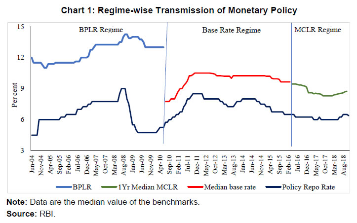 The focus of the study is to estimate the degree of monetary policy pass-through to domestic banks’ lending rates during the latter half of Base Rate regime (Q4:2012-13 to Q4:2015-16) and MCLR regime (Q1:2016-17 to Q2:2018-19). IV.1 Aggregate Analysis Before examining the pass-through of monetary policy to individual banks’ lending rates, we analyse the same at the aggregate level for the entire period under study. Here, we consider four variables, viz. the weighted average lending rate on fresh rupee loans sanctioned by domestic banks (walrf), monetary policy variable – weighted average call rate (wacr), inflation and real GDP. Our main objective is to verify the impact of monetary policy changes (wacr) on walrf. Inflation and real GDP are the control variables of the model. We examined the impact in a VAR framework, for which impulse response function has been estimated. As per the Augmented Dickey-Fuller (ADF) test, all the variables were found to be I(1). Then we examined if the variables are cointegrated. Accordingly, we checked the long-run relationship using Johansen cointegration model. The idea is if they are cointegrated then we go for Vector Error Correction (VECM) model estimation and if they are not cointegrated, then we adopt VAR model. The Johansen cointegration test results are given below in Table 2. Results of the Johansen cointegration test show that there exists a cointegrating relation as per both the trace test and the maximum eigenvalue test, under the 5 per cent significance level. In other words, there is a stable long-term equilibrium relationship among the variables. We now run the Vector Error Correction Model (VECM) to examine both the short-run and long-run dynamics of the series. Conventional ECM for cointegrated series are:  where, zt-1 is the error correction term and is the OLS residual from the following long-run cointegrating regression:  and is defined as  The coefficient of ECT, φ, is the speed of adjustment, because it measures the speed at which y returns to equilibrium after a change in x. It is observed from Table 3 that the relationship between walrf of domestic banks and wacr is positive and statistically significant at 1 per cent level of significance. From the long run equation of cointegrated model, we can infer that a 1 percentage point increase in the walr leads to a 0.36 percentage point increase in the walrf (Table 3 and Chart 2). It is our contention, however, that there is considerable heterogeneity among banks in passing on the monetary impulses to their respective lending rates driven by bank-specific factors. Therefore, it is prudent to estimate the impact of a policy shock in the ΔWACR based on a dynamic panel data regression model (GMM model) controlling for this heterogeneity. The remainder of this paper focuses on the disaggregated level, which is discussed in the following section.
 IV.2 GMM Model Banks typically determine their interest rates on deposits and loans in an oligopolistic market setting (Santomero, 1984; Gambacorta, 2008). Banks are, therefore, not price-takers but price their loans depending on both macroeconomic and microeconomic (i.e., individual bank-specific) factors - the latter including cost of funds, operating costs, asset quality, etc. Since the main objective of this study is to assess the nature of transmission of the change in the monetary policy rate to the lending rates of individual banks under different interest rate benchmarks, we have introduced some control variables in the model. Apart from bank-specific characteristics, inflation and real GDP are also included as control variables in the study. Against this backdrop, we estimate the following equation to examine the monetary transmission process: 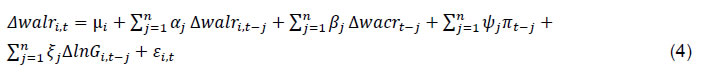 and 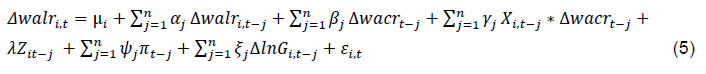 where, i = 1…. N; j = 1...n; and t = 1 …. T; where N = number of banks; n = the number of lags in the model, Here equation (4) represents the benchmark model without inclusion of any bank-specific variables and equation (5) represents the model including bank-specific characteristics. The selection of instruments is done based on diagnostic tests (viz., AR(1), AR(2) and Sargan). We have added real GDP growth and inflation in the model to control for the demand effects [Ehrmann et al. (2001), Gambacorta (2001), Holton et al. (2018)].4 Since all the variables in level are integrated of order one, we have taken the difference of the variables in our model (Appendix Table A). All the data were seasonally adjusted to take care of the seasonality aspect. The above model would have been appropriate if wacr was the proxy for the repo rate for the entire period. However, during Q2 and Q3:2013-14, the marginal standing facility (MSF) rate had become the de facto policy rate supplanting the repo rate. This happened when responding to the hurried flight to safety by FIIs following the Fed announcement on withdrawal of the stimulus, the RBI raised the MSF rate to defend the exchange rate even as the repo rate – a tool to indicate the monetary policy stance on domestic price stability – was left unchanged resulting in a spread of 300 bps between the MSF rate and the repo rate (from 100 bps earlier). As liquidity tightening measures were also taken, wacr shot up and remained aligned to the MSF (instead of the repo rate) during this period. Once normalcy was restored in the financial markets, MSF rate was reduced; while simultaneously, the repo rate had to be raised to contain the inflationary pressures resulting in a peculiar situation of the wacr declining even as the repo rate was rising. In equation (4), therefore, we have introduced a dummy variable D1 for the two quarters (2013-14: Q3 to 2013-14: Q4) to capture the impact of taper tantrum on walr. We also introduce the dummy D2 for 2016-17: Q3 to 2017-18: Q1 to capture the demonetization effect on WALR. After the introduction of the dummy variable, our model becomes: 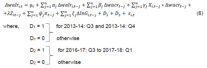 Consistent with the literature5, the bank-specific characteristics have been reparametrized in the following way:  where, Xi,t is the normalised bank-specific characteristic explained later. Here ϕi,t is observation of ith bank in period t and Nt is the total number of banks in period t. Further, T is the total number of periods. That means each observation of a particular bank for period t is normalised with respect to the number of banks and number of periods. In other words, each indicator/ bank-specific characteristic is normalised with respect to the averages across all the banks in the respective sample so that the sum over all observations becomes zero. Since the average of the interaction term between the monetary policy variable (Δwacrt-j) and Xi, t-j in equation (4) is zero for the average bank, the parameters βj can be directly interpreted as average monetary policy effect [Ehrmann et al. (2001), Gambacorta (2001), Holton et al. (2018)]. Since there is heterogeneity in interest rate pass-through across the whole banking system, each variable is required to be normalised with respect to the average across all banks in each period of time. Following Gambacorta (2001), we have normalised the size indicator in respect of both - the mean over the whole sample period as well as for every single period - to remove the unwanted trends6. Dependent Variable To measure the impact of pass-through under different regimes, we use the q-o-q change in the weighted average lending rate (walr) on fresh rupee loans sanctioned by banks during the month as the dependent variable. Fresh rupee loans have been preferred as the dependent variable to outstanding rupee loans as the former is priced with reference to the prevailing benchmark, unlike outstanding rupee loans which have a sizeable share of loans priced to the earlier benchmark(s). Independent variables The objective of this study is to examine the relationship between a monetary policy indicator and lending rates. Instead of the policy repo rate, we have used the weighted average call money rate (wacr), which is the operating target of monetary policy and mimics the policy repo rate as the indicator of monetary policy stance in our model: the correlation coefficient between the two was found to be as high as 0.94 for the period under study (March 2013 - September 2018). While the repo rate depicts a step-wise movement, the wacr fluctuates daily also, reflecting the liquidity condition in the system and thus, better reflects the overall stance of monetary policy. We include two important macro variables - CPI inflation and real GDP growth - as controls in our regression model. These variables capture the risk of lending to certain markets and the demand for credit, respectively. According to Holton et al. (2018), there is no clear-cut direction of the effect of CPI inflation and real GDP growth on the interest rates. The relationship between each of the macro variables and wacr can be either negative or positive depending on the dominance of demand or risk. When growth is decelerating (and inflation declining) accompanied by declining credit demand, we may expect lending rates to fall. However, a slowdown in real economic activity (accompanied by a decline in inflation) may damage borrowers’ creditworthiness resulting in a rise in risk premia, thereby raising their cost of borrowings. Bank-level variables Pricing of loans extended by a bank depends on bank-specific characteristics. In each of the 9 models, we have used a unique bank-specific variable: term deposit rate, total asset size, liquidity, capital to risk-weighted assets ratio (CRAR), return on assets, non-performing assets, non-interest income, operating expenses and investments in securities approved for statutory liquidity ratio (SLR). The rationale behind choosing these variables is detailed below. Bank deposits are one of the most important components of funding in India. In a cost-plus pricing structure, a direct relationship between the cost of funding and lending rates is expected. However, the deposit rate may not respond 1-1 to the change in monetary policy, impeding transmission to lending rates.7 There is a contrasting view on the relationship between the size of bank assets and the lending rate. Maudos and De Guevara (2004), Angbazo (1997) found a negative relationship between bank size and net interest margins (interest income minus interest expenditure). Holton et al. (2018) reported that an increase in the size of the bank leads to a decrease in the overall pass-through of money market rate. Sensarma and Ghosh (2004) found that there is a significant positive relationship between the size of Indian banks and NIM. Further, John et al. (2018) reported contrasting results for bank groups in India depending on the chosen time period. Liquidity is considered as a barometer to measure the balance sheet condition of a bank; it also influences the degree of pass-through (Holton et al., 2018). Bluhm et al. (2014) found that banks with illiquid assets were subjected to shocks during a crisis and compelled to deleverage. Gambacorta and Mistrulli (2011) showed that banks with liquid assets transmit more in response to monetary policy during an expansionary phase. Capital to Risk-Weighted Asset Ratio (CRAR) is the ratio of a bank's capital in relation to its risk-weighted assets. Scheduled commercial banks in India are required to maintain a CRAR of 9 per cent8. Prudent banks may prefer to maintain additional capital over and above the regulatory requirements to meet unanticipated future requirements in an uncertain market environment, which could impede monetary transmission during the expansionary phase (Behera et al., 2020). Since higher CRAR raises costs of intermediation, we expect that banks will pass on the higher costs to their lending rates. In case of return on assets (RoA), the relationship between the lending rates and RoA is not linear; it depends on the monetary policy cycle, the health of the bank balance sheet and whether the bank is driven by the objective of maximisation of profits or sales. For example, a bank with a stronger balance sheet and a higher RoA may be motivated to capture a higher market share irrespective of the policy cycle; hence, it may lower its lending rates faster vis-à-vis its competitors during an easing cycle but may not increase its lending rates during tightening of monetary policy. Therefore, the relationship between the two is not clear-cut. Regarding asset quality, a high degree of non-performing assets may prompt reduced pass-through. This is exactly corroborated by the empirical literature (Holton et al., 2018). In the Indian case, John et al. (2018) have found that deterioration of asset quality impacted monetary transmission. Non-interest income (NII) is an increasingly important source of income for banks. Banks look at the totality of income – interest and non-interest - from a customer. Banks may aim at expanding their customer base by providing loans at a lower rate of interest to those providing fee-based income to banks to maximise their total income (Dumicic and Ridzak, 2013; Moudos and Solis, 2009; Carbo and Rodriguez, 2007, John et al., 2018). We may, therefore, expect a negative relationship between the non-interest income and lending rates of banks. Operating expenses are expenses in relation to the operations of a business on a daily basis. Various components such as salaries and pensions, administrative expenses, software costs, occupancy costs, etc. come under this head (John et al., 2018; Dumicic and Ridzak, 2013). There is an agreement in the literature that banks normally transmit the burden of operating costs to the customer. This is feasible in an oligopolistic setting. However, where banks are driven by considerations of social banking or where the majority owner itself has considerations other than profit maximisation, a negative relationship between operating costs and lending rates could be observed. Further, when banks already earn a very high NIM, they may have the leeway to absorb the rise in operating costs and not pass it on to their customers. Even when a bank prices its loans off an internal benchmark, which has operating cost as one of its components, the bank can reduce the spread it charges over the benchmark to prevent the lending rate charged to the customer from rising to the full extent of the rise in operating costs. In view of this, we may not expect an unambiguous relationship between the lending rates and operating expenses. Another measure of liquidity is investments in approved securities to maintain the statutory liquidity ratio (SLR). Investments in approved securities over and above SLR can be used for availing liquidity.9 An individual bank with more liquid assets may be able to offload the securities to fund credit growth while efficiently transmitting policy rate signals during an easing phase. However, when the overall SLR in the banking system is high and banks are unable to offload the securities to fund credit demand without booking losses, credit may get crowded out and transmission to lending rates impeded. Estimation For our estimation, we have used system GMM dynamic panel data model developed by Arellano and Bond (1991) and Arellano and Bover (1995). The rationale for choosing GMM/ instrumental variables (IV) method for our empirical exercise is that it addresses various pitfalls associated with the least square based inference methods when the model is dynamic, i.e., dependent variable (in our case walr) is regressed on its past values (Bun and Sarafidis, 2015). In such a case, when lagged dependent variables are taken on the right-hand side of the equation, the problem of endogeneity emerges. Arellano-Bover (1995) method resolves this problem by including instrumental variables (IV) in the equation. Further, it also ensures efficiency and consistency of the estimates as compared with the least squares-based inference methods, provided that the model is not subject to a serial correlation of order two and that the instruments used are valid (Gambacorta, 2008). While the validity of the instruments (over-identification of the model) is tested with the help of Sargan test, serial correlations of the residuals are tested with the help of A-B serial autocorrelation (AR1 and AR2) test in residuals for the first order and second order.10 The use of lagged values of dependent and explanatory variables as IVs is crucial to avoid endogeneity problems. For example, real GDP growth and CPI inflation not only determine the loan demand, they determine the policy rate as well. In our econometric exercise, we have chosen appropriate lags and dropped the insignificant lagged variables. The data set has been seasonally adjusted to remove the seasonality bias. Our analysis is based on all the domestic (public and private sector) banks. The study has been conducted by taking bank-specific data of individual banks. All the bank-specific data have been collected from the Reserve Bank. The remaining data have also been collected from RBI publications, such as the Handbook of Statistics on India, Statistical Tables relating to Banks in India and Database on Indian Economy. A summary of statistics in respect of the base rate and MCLR regimes is presented in Table 411. Following are the highlights from the table: The size of the banks increased over time (in nominal terms), while the return on assets declined sharply. Non-performing assets of banks increased sharply following the asset quality review (AQR), which coincided with the introduction of the MCLR regime. Operating expenses remained unchanged throughout the period. Non-interest income was 10.4 per cent of total income in the base rate period and increased to 13.6 per cent in MCLR regime. Surplus liquidity in the banking system was higher during the MCLR regime. CRAR changed marginally - increasing from 12.4 per cent during the base rate period to 12.6 per cent in the MCLR regime. We have estimated Equation (4) by using the system GMM as suggested by Arellano-Bover (1995). GMM is efficient when N (number of cross-sections – banks in our case) is large and T (time period) is small. Accordingly, it is appropriate to use GMM. We have used the test statistics in our results as diagnostic tests. The regression results are presented in Tables 5-8 for the whole period and the two sub-periods as discussed earlier12. It may be stated that although we included GDP growth in our model at the beginning, subsequently, we dropped the variable, since the inclusion of growth creates multicollinearity problem when dummy variables are introduced. Following Ehrmann et al. (2003) and Gambacorta (2008), we discuss the estimated long-run coefficients only. Table 5 depicts the benchmark regressions results without the addition of any bank-specific characteristics as shown in equation (4). It is observed that a 1 percentage point change in the wacr leads to 0.12 percentage point change in walrf in the same direction for the whole sample in the long run, while the figures are 0.12 percentage point and 0.21 percentage point, respectively, in case of base rate and MCLR regimes. Thus, the impact of monetary policy on walrf is more during the MCLR regime in comparison to the base rate regime in benchmark regressions. The impact of inflation on lending rates is statistically significant and on expected lines. V.1 Whole Sample: 2012-13: Q4 to 208-19: Q2 In this sub-section, we introduce the nine bank-specific characteristics and the interaction term of the monetary policy indicator (wacr) with each of these characteristics separately to estimate equation (5) in Models 1-9 for the entire sample period. The introduction of the interaction terms is to estimate the influence of each bank-specific characteristic on the lending rate (walrf) for any change in the wacr. These variables have been re-parameterised such that yj in equation (5) can be interpreted as average effect. The results for the whole sample in Table 6 indicate that the long-run effect of wacr on lending rates is significantly different from zero in all the models. Further, the estimated long-run multipliers of wacr have the expected positive sign and are significantly different from zero in all models. The estimates imply that a 1 percentage point increase/decrease in the wacr leads to an increase/decrease in the walrf by 0.13-0.24 percentage point in the long run (Models 1-9). On the effects of inflation on lending rates, the long run relationship is positive and statistically significant in all cases except one. The coefficient of the interaction term between the term deposit rate (watdr) and wacr (Model 1) is significant and positively related, implying higher the deposit rate, the higher is the lending rate, which is in line with our expectations. The coefficient of the interaction term between size and wacr (Model 2) is significant and positive. This implies that a larger-sized bank increases its lending rate when there is an increase in wacr and vice versa. In the case of CRAR, the relationship is significant and negative. This implies that banks with higher CRAR provide credit at a lower rate in response to the easing of monetary policy. In the case of operating expenses, the relationship is significant and positive. This indicates that banks with higher operating expenses provide credit at a higher lending interest rate irrespective of the stance of monetary policy. This is in line with our expectations. That means, higher operating expenses hinder the transmission mechanism of monetary policy during an easing phase. The interaction terms for the remaining five variables are observed to be statistically insignificant.
In our sample, the base rate regime covers the period from 2012-13:Q4 to 2015-16:Q4. The results for this period reported in Table 7 show that 1 percentage point change in wacr leads to change in the walrf in the range of 0.22-0.35 percentage point after one quarter (lagged coefficient). And the relationship is observed to be statistically significant in all the cases. Regarding the long-run relationship, the effect of change in wacr on change in walrf is significantly different from zero in all the 9 models. Further, the long-run coefficients of wacr have the positive sign as expected. The estimates indicate that a 1 percentage point increase in the monetary policy indicator (wacr) leads to an increase in the walrf of 0.11-0.19 percentage point in the long run. On the effects of macroeconomic variables (i.e., inflation), banks expectedly raise their lending rates in an inflationary situation. The coefficients of the interaction terms between wacr and CRAR (Model 4), and NII (Model 7) are found to be statistically significant at conventional values. Thus, the results indicate that banks with higher CRAR charge lower lending rates, as observed in the whole sample period. The sign of the CRAR is against our expectations. Higher capital motivates banks to decrease their lending rates, thereby facilitating the transmission process during the easing cycle. In the case of NII, monetary transmission is hindered by the high non-interest income during the easing cycle: this is because when the banks’ non-interest income is high, they appear to be reluctant to reduce their lending rates in response to the reduction of the policy rate. The coefficients of the interaction terms between the remaining seven bank-specific indicators and wacr are statistically insignificant at the conventional level.
V.3 MCLR Regime The MCLR regime covers the period from 2016-17:Q1 to 2018-19:Q2. The results including their statistical significance vary across models 1-9 (Table 8). The long-run coefficients of wacr have the positive sign as per expectations and are statistically significant in all the models. The estimates show that a 1 percentage point increase/decrease in the monetary policy indicator (wacr) leads to an increase/decrease in the lending rate (walrf) by 0.26-0.47 percentage point in the long run, which is more than that during the base rate regime for each of the models. This is notwithstanding the worsening in the bank balance sheets during the MCLR regime when one would have expected banks to load risk premia onto their lending rates impeding transmission; besides, monetary policy was undergoing an easing cycle (except for 2018-19:Q2), when the speed of transmission to lending rates is usually lower (Singh, 2011; RBI, 2011). Since the demonetiation dummy was not significant, we could not conclude that transmission during the MCLR regime was facilitated by demonetisation, which was independent of monetary policy. As in the case of the whole sample period, in some cases, the long-run coefficients are lower than the sum of the lagged coefficients for monetary policy during MCLR regime.13 On the effects of macroeconomic variables, an increase in inflation expectedly leads to an increase in lending rates of banks, similar to our findings in case of the whole sample period and base rate regime. The coefficient of the interaction terms with the monetary policy indicator (wacr) are found to be statistically significant in case of four models, viz., deposit rate (Model 1), size (Model 2), liquidity (Model 3) and NPA (Model 6). Except for the sign of the coefficient for NPAs, the other three are on the expected lines. In other models, the coefficients of the interaction terms are insignificant. From the results, the following inference can be drawn. The coefficient of the interaction term between the deposit rate (watdr) and wacr (Model 1) is statistically significant and positively related, implying higher the deposit rate, higher is the lending rate, which is in line with our expectations. Further, as in the whole sample period, higher the size, higher is the lending rate. That means, during the easing cycle transmission process is hampered since banks do not reduce their lending rates in response to reduction in policy rate. Second, due to the existence of excess liquidity in the banking system, walr declined more in response to the reduction in the policy rate. Lastly, unlike the Base Rate regime, we observe a negative significant relationship between NPA and wacr in the MCLR regime; hence higher the NPA, lower is the walr, which is against our expectations, but consistent with the findings of John et al. (2018). If banks were to price in risk premia to their lending rates, one would have expected a positive correlation; the negative relationship could perhaps be attributed to the risk averse strategy adopted by many banks following the introduction of Asset Quality Review (AQR) that resulted in a spurt in NPAs; several banks were also barred from risky lending under the prompt corrective action (PCA) framework. As a result, banks altered their lending strategy to focus more on collateralised retail loans like housing and vehicle financing where lending rates are typically lower than other sectors because of lower default risk and greater competition with many non-bank players in the credit market (RBI, 2019).
VII. Conclusion In a bank-dependent economy, efficient monetary policy transmission to banks’ lending rates is a crucial conduit for the successful implementation of monetary policy. However, transmission from policy rate to lending rates has remained partial. To mitigate this problem and ensure customer protection, the Reserve Bank has changed the lending rate benchmark over time since the deregulation of lending rates in October 1994. Against this backdrop, this study has attempted to compare the degree of transmission to the walr charged by individual banks between the two interest rate benchmark regimes – base rate and MCLR - following a change in the monetary policy rate. In our study, we have considered three different time periods, viz., whole sample period (i.e., Q4:2012-13 to Q2:2018-19) and its two sub-periods - base rate regime (i.e., Q4:2012-13 to Q4:2015-16) and MCLR regime (Q1:2016-17 to Q2:2018-19). We have used GMM model suggested by Arellano-Bover (1995) to estimate the equations for the whole sample and the two sub-periods. For each time period, we have estimated the benchmark regression followed by 9 models - each incorporating a unique bank-specific characteristic. In order to provide a reference for drawing a comparison with the individual models in a GMM framework, we have run a VEC model by taking the aggregate level time series data, since data were found to be I(1) and also co-integrated. From the VECM results, we find that there is a change in weighted average lending rate on fresh rupee loans (walrf) of domestic banks of 0.36 percentage point due to a 1 percentage point shock in the wacr – the proxy for the monetary policy rate. After doing the VECM analysis, we have focused on the bank-level data in a panel data set-up. Thus, from the GMM results, we observed that for the whole sample period, the long-run coefficients of wacr on walr are significant in all the models and have the expected positive sign. It is estimated that a 1 percentage point increase in the wacr leads to an increase in the walrf ranging 0.13–0.24 percentage point in the long-run depending on which one of the nine different models is chosen. An increase/decrease in inflation expectedly leads to an increase/decrease in lending rate; our findings are similar in this regard for the two sub-periods. Among the bank-specific characteristics, the coefficient of the interaction term with wacr were found to be statistically significant at conventional values for watdr, size, CRAR and operating expenses. Thus, a rise in the watdr (or size) of banks leads to an increase in the lending rate. This means that when the wacr increases, walr increases because of an increase in the watdr (or size). During the easing phase, on the other hand, walr declines in response to a decline in the wacr; however, walr may not decline proportionately because of higher watdr, which hinders effective monetary transmission. Monetary transmission is, therefore, stronger during the tightening period as compared with the easing phase. In the case of model with size, when the call rate declines, the lending rate declines; but due to bigger size of the bank, lending rate does not decline commensurate with decline in the call rate. Hence, monetary transmission is adversely affected during the easing cycle of monetary policy. CRAR is the third variable for which we have found a statistically significant and negative relationship between wacr and CRAR. This implies that banks with higher CRAR lower their lending rate. Hence, bank recapitalisation would facilitate transmission during the easing phase as higher capital enables banks to overcome statutory restrictions and increase lending by lowering their lending rates. Operating cost is the fourth variable for which a positive and significant relationship was found, implying that a rise in operating costs hinders transmission during the easing phase. For the 1st sub-period, a 1 percentage point increase/decrease in the wacr led to an increase/decrease in the walrf of 0.22-0.35 percentage point for a typical bank in the long run. The coefficients of the interaction term with wacr and two bank-specific variables viz., CRAR and NII were statistically significant, but not in the same direction. In case of CRAR, we have found a significant negative relationship as found in the whole sample period. In case of the model incorporating NII, although the walrf declines in response to a decline in wacr, the extent of decline gets partly offset when the non-interest income is large. That means the transmission is impeded during the easing cycle due to increased non-interest income. For the 2nd sub-period, i.e., during the MCLR regime, a 1 percentage point increase in the wacr leads to an increase in walrf of 0.26-0.47 percentage point in the long run. For all models, transmission is more during the MCLR regime than the base rate regime. The interaction term between wacr and four of the 9 bank-specific variables – deposit rate, size, liquidity, and NPA - is significant. The signs of the coefficients are on the expected lines for three of the variables viz., deposit rate, size, and liquidity. In the case of the deposit rate, it is observed that the higher the deposit rate, the higher is the lending rate, as observed in the case of both the whole sample period. Theoretically, it is consistent since a rise in the deposit rate may lead to a concomitant increase in the cost of funds. Therefore, due to the rise in the cost of funds, banks will pass on this cost to the lending rate, which we observe from our findings. In the case of size, it is observed that the higher the size, the higher is the lending rate, as observed in the case of both whole sample periods. Liquidity has a negative and significant relationship with the lending rate, implying that the walrf cannot increase commensurately with the rise in wacr in a tightening phase in the presence of higher availability of surplus liquidity in the system. Also, excess liquidity acts as a facilitator of monetary transmission during the easing phase. A major finding of the study corroborating other studies is that during the MCLR regime, banks could not price credit to reflect the sharply rising NPAs in their balance sheet following the AQR. Faced with higher NPAs prompting the tightening of regulatory norms by RBI and risk-averse strategy adopted by banks, banks were unable to increase their walrf on the aggregate lending portfolio even as credit growth decelerated sharply. Since banks did not enjoy maneuverability in the pricing of loans when NPAs rose sharply, transmission did not get obstructed during the easing regime. To conclude, irrespective of the model chosen, transmission is higher during the MCLR regime than the Base Rate regime. Furthermore, the synchronising of liquidity management with the monetary policy stance, introduction of the flexible inflation targeting (FIT) framework coupled with the deceleration in economic activity reducing credit demand could be contributory factors for better transmission during the MCLR regime. Nevertheless, transmission during the MCLR regime was far from satisfactory necessitating the introduction of external benchmark-based pricing of loans for the personal loans and micro & small enterprises, effective October 1, 2019, and for medium enterprises since April 1, 2020. The progressive shift from the various internal benchmark-based pricing of loans to the external benchmark augurs well for monetary transmission going forward. @ Sadhan Kumar Chattopadhyay (skchattopadhyay@rbi.org.in) is Director in the Department of Economic & Policy Research and Arghya Kusum Mitra (akmitra@rbi.org.in) retired as Director in Monetary Policy Department, Reserve Bank of India. * The views expressed in the paper are those of the authors and do not represent the views of the institution they are affiliated with. The authors gratefully acknowledge the encouragement received from Michael Debabrata Patra to conduct this study. The authors are thankful to Mridul Kumar Saggar, Muneesh Kapur, Joice John, Harendra Behera, Pranab Kumar Das (CSSS, Kolkata) and Samarjit Das (ISI, Kolkata) for their valuable comments/suggestions; and to Angshuman Hait and Suvendu Sarkar for making the data available for the study. Insightful comments from Pratik Mitra, an anonymous referee and participants of the DEPR Study Circle seminar in improving the content of the paper are gratefully acknowledged. 1 In 2000, the Reserve Bank allowed external benchmark-based pricing of loans by banks to run in parallel with internal benchmark-based pricing of loans; banks, however, almost always chose the latter. 2 We have excluded foreign banks operating in India because they account for less than 5 per cent of bank credit extended by scheduled commercial banks (although the number of foreign banks is more than that of public and private sector banks combined) and their business strategy (i.e., funding sources and nature of lending operations) is different from that of domestic banks. 3 Data are seasonally adjusted since they are quarterly data. 4 As stated by Gambacorta (2004), “The introduction of these two variables allows us to capture cyclical movements and serves to isolate the monetary policy component of interest rate changes.” 5 Please see Gambacorta (2001, 2008), Ehrmann, et al. (2003), Holton, et al. (2018). 6 Unwanted trend in size occurs as size is measured in nominal terms. 7 Longer maturity fixed rate term deposits, rigid saving deposit rates (banks kept their saving deposit rate unchanged from October 2011 to June 2017 irrespective of the monetary policy cycle), dependence on retail term deposits to meet their funding requirements keep their funding costs relatively rigid (Mitra and Chattopadhyay, 2020; Kumar et al., 2021; Kumar et al., 2022). The problem is typically compounded by higher small saving rates than bank term deposit rates, particularly during easing cycles. 8 Details are available in Behera et al. (2020). 9 Banks are even permitted to dip into their excess SLR to fund their temporary liquidity mismatches 10 As per the Arellano-Bond test, the first order autocorrelation should be negative and significant and the second and higher order autocorrelation should be insignificant (John et al., 2018). 11 Since comparable data under BPLR regime are not available, we have excluded the BPLR regime in the model. 12 Due to paucity of data, we could not conduct non-linearity test, which would have been useful. 13 Here the models are valid only with zero lag. Accordingly, no lag has been used in this case. References: Abuka, C., Alinda, R. K., Minoiu, C., Peydró, J., & Presbiter, A. F. (2019). Monetary policy and bank lending in developing countries: Loan applications, rates, and real effects. Journal of Development Economics, 139:185-202. Acharya, V., Imbierowicz,V. B., Steffen, S., & Teichmann, D. (2020). Does the lack of financial stability impair the transmission of monetary policy? Journal of Financial Economics, https://doi.org/10.1016/j.jfineco.2020.06.011. Aleem, A. (2010). Transmission mechanism of monetary policy in India. Journal of Asian Economics, 21(2): 186-197. Al-Mashat, R. (2003). Monetary Policy Transmission in India - Selected Issues. IMF Staff Country Report, 03/261 (Washington: International Monetary Fund). Altavilla, C., Canova, F. & Ciccarelli, M. (2016). Mending the broken link: heterogeneous bank lending and monetary policy pass-through. Working Paper Series No. 1978, European Central Bank. Ando, A., & Modigliani, F. (1963). The ‘life-cycle’ hypothesis of saving: aggregate implications and tests. American Economic Review, 53: 55–84. Angbazo, L. (1997), “Commercial Bank Net Interest Margins, Default Risk, Interest-rate risk, and Off-balance Sheet Banking”, Journal of Banking and Finance, Vol. 21, pp. 55-87. Angelini, P. (2018). Do high levels of NPLs impair banks’ credit allocation? Notes on Financial Stability and Supervision, No. 12, Banca d’ Italia, April. Arellano, M. and O. Bover (1995). Another Look at the Instrumental Variable Estimation of Error Components Models. Journal of Econometrics, 68: 29-5.1 Arellano, M. and S.R. Bond (1991), Some tests of specification for panel data: Monte Carlo evidence and an application to employment equations, Review of Economic Studies, 58: 277-297. Bennouna, H. (2018). Interest Rate Pass-through in Morocco: Evidence from Bank-level survey data. Economic Modeling. https://doi.org/10.1016/j.econmod.2018.11.003. Bernanke, B. & Gertler, M. (1995). Inside the black box: the credit channel of monetary transmission. Journal of Economic Perspectives, 9: 27-48. Bernanke, Ben S. & Blinder, A. S. (1988). Credit, money, and aggregate demand. American Economic Review Papers and Proceedings, 78: 435-439. Bhattacharya, R., Patnaik, I., & Shah, A. (2010). Monetary policy transmission in an emerging market setting. IMF Working Paper, WP/11/5. Bhaumik, S. K., Dang, V., & Kutan, A. M. (2011). Implications of bank ownership for the credit channel of monetary policy transmission: Evidence from India. Journal of Banking & Finance, 35 (2011): 2418–2428. Bhoi, B.K., Mitra, A. K., Singh, J. B. & Gangadaran, S. (2017). Effectiveness of alternative channels of monetary policy transmission: some evidence for India. Macroeconomics and Finance in Emerging Market Economies, 10(1):19-38, DOI: 10.1080/17520843.2016.1188837. Bluhm, M., Faia, E., Krahnen, J.P. (2014). Monetary Policy Implementation in an Interbank Network: Effects on Systemic Risk. Technical Report. Bun, Maurice J. G. & Sarafidis, V. (2015). Dynamic Panel Data Models. In B. H. Baltagi (Ed.), The Oxford Handbook of Panel Data. Carbo V.S., and Rodriguez, F. F. (2007), “The Determinants of Bank Margins in European Banking”, Journal of Banking and Finance, 31(7), p. 2043-2063. Cecchetti, S. G., Kohler, M., & Upper, C. (2009). Financial crises and economic activity. Paper presented at Jackson Hole Symposium Wyoming, August 10-11. Das, Sonali. (2015). Monetary Policy in India: Transmission to Bank Interest Rates. IMF WP No. 15/129. Das, T. B. (2013). Net Interest Margin, Financial Crisis and Bank Behaviour: Experience of Indian Banks. RBI Working Paper Series: 10, October. Dumicic, M., and T. Ridzak (2013). Determinants of banks’ net interest margins in Central and Eastern Europe. Financial Theory and Practice 37(1):1-30 Edwards, F., & Mishkin, F. S. (1995). The decline of traditional banking: implications for financial stability and regulatory policy. NBER Working Papers No. 4993, National Bureau of Economic Research. Ehrmann M., Gambacorta L., Martinez Pagés J., Sevestre P., & Worms, A. (2001). Financial Systems and the Role of Banks in Monetary Policy Transmission in the Euro Area in Angeloni I., Working Paper Series, ECB. Working paper No. 105, December. Ehrmann M., Gambacorta L., Martinez Pagés J., Sevestre P., & Worms, A. (2003). Financial Systems and the Role of Banks in Monetary Policy Transmission in the Euro Area. In Angeloni I., Kashyap A. and Mojon B. (Ed.), Monetary Policy Transmission in the Euro Area. Cambridge University Press. Cambridge. Friedman, M., & Schwartz, A. J. (1963). A monetary history of the United States, 1867-1960. Princeton University Press. Gambacorta L. (2001). Bank-specific characteristics cteristics and monetary policy transmission - the case of Italy. Working Paper Series, ECB. Working paper No. 103, December. Gambacorta, L. (2004). Does bank capital affect lending behavior? Journal of Financial Intermediation, 13 (4): 436-457. Gambacorta, L. (2008). How do banks set interest rates? European Economic Review, 52 (5): 792–819. Gambacorta, L. and H. S. Shin. (2018). Why bank capital matters for monetary policy. Journal of Financial Intermediation, 35:17-29. Gambacorta, L., and P. E. Mistrulli. (2011). Bank heterogeneity and interest rate setting: what lessons have we learned since Lehman Brothers? Temi di discussion (Economic working papers) 829. Bank of Italy. Economic Research and International Relations Area. Ghosh, S., A. Narayanan and P. Garg. (2021). Monetary Policy Transmission in India: New Evidence from Firm-Bank Matched Data. RBI Working Paper Series, WPS (DEPR): 01 / 2021. Gomez, M., Landier, A., & Sraer, D. (2020). Banks’ exposure to interest rate risk and the transmission of monetary policy. Journal of Monetary Economics. https://doi.org/10.1016/j.jmoneco.2020.03.011 Holton, S., & D’Acri, C.R. (2018). Interest rate pass-through since the euro area crisis. Journal of Banking and Finance. 96, 277-291. John, J., Mitra, A. K., Raj J., & Rath, D. P. (2018). Asset Quality and Monetary Transmission in India. Reserve Bank of India Occasional Papers, 37(1&2), 2016. Kapur, M. and Behera, H. (2012). Monetary Transmission Mechanism in India: A Quarterly Model. RBI Working Paper Series, WPS (DEPR): 09/2012. Keynes, J. M. (1936). The general theory of employment, interest and money. New York: Harcourt, Brace. Khundrakpam, J. K. (2011). Credit Channel of Monetary Transmission in India - How Effective and Long is the Lag? RBI Working Paper Series, WPS (DEPR): 20/2011. Khundrakpam, J. K., & Jain, R. (2012). Monetary Policy Transmission in India: A Peep Inside the Black Box. RBI Working Paper Series, WPS (DEPR): 11/2012. Kumar, A., Prakash, A and Latey, S. (2022), Monetary Transmission to Banks’ Interest Rates: Implications of External Benchmark Regime. RBI Bulletin, July 2021, Volume LXXVI Number 4. Kumar, A. and P. Sachdeva. (2021). Monetary Policy Transmission in India: Recent Developments. RBI Bulletin, July 2021, Volume LXXV Number 7. Mahathanaseth, I. and Tauer, L. W. (2018), Monetary policy transmission through the bank lending channel in Thailand. Journal of Asian Economics, Xxx, xxx–xxx. María C.S., Azofra, S. S., Olmo, B.T. & Gutiérrez, C.L. (2018). A new approach to the analysis of monetary policy transmission through bank capital. Financial Research Letters, 24: 95-104. Maudos, J. and J. F. de Guevara. (2004). Factors Explaining the Interest Margin in the Banking Sectors of the European Union. Journal of Banking & Finance 28(9):2259-2281. Maudos, J., and L. Solis. (2009).The determinants of net interest income in the Mexican banking system: An integrated model. Journal of Banking & Finance, 2009, vol. 33, issue 10, 1920-1931. Meltzer, A. H. (1995). Monetary, credit and (other) transmission processes: a monetarist perspective. Journal of Economic Perspectives, 9: 49-72. Mishra, A. and Kelly Burns b. (2017), The effect of liquidity shocks on the bank lending channel: Evidence from India. International Review of Economics and Finance, 52 (2017): 55–76. Mishra, P., Montiel, P., & Sengupta, R. (2016). Monetary Transmission in Developing Countries: Evidence from India. Indira Gandhi Institute of Development Research, Mumbai March. Mishra, P., Montiel, P. J., & Spilimbergo, A. (2010). Monetary transmission in low income countries. CEPR Discussion Paper No. DP7951. Mitra, A.K. and Chattopadhyay, S.K. (2020). Monetary Policy Transmission in India – Recent Trends and Impediments”, Reserve Bank of India Bulletin, March 2020. Volume LXXIV Number 3. Mohanty, D. (2012). Evidence of Interest Rate Channel of Monetary Policy Transmission in India. RBI Working Paper Series, WPS (DEPR): 06/2012. Mohanty, M. S., & Turner, P. (2008). Monetary policy transmission in emerging market economies: what is new? BIS Papers No.35, Bank of International Settlements. Muduli, S., & H. Behera. (2020). Bank Capital and Monetray Policy Transmission in India. RBI Working Paper Series, WPS (DEPR): 12/2020. Mukherjee, S., & Bhattacharya, R. (2011). Inflation targeting and monetary policy transmission mechanisms in emerging market economies. IMF Working Paper No. WP/11/229, International Monetary Fund. Obstfeld, M. & Rogoff, K. (1995). The mirage of fixed exchange rates. Journal of Economic Perspectives, 9: 73-96. Pandit, B.L., Mittal, A, Roy, M., Ghosh, S. (2006). Transmission of Monetary Policy and the Bank Lending Channel: Analysis and Evidence for India. DRG Study, No. 25, RBI. Pandit, B. L. & Vashisht, P. (2011). Monetary Policy and Credit Demand in India and Some EMEs. ICRIER WP, 256. Patra, M.D. and Kapur, M. (2012), “A Monetary Policy Model for India”, Macroeconomics and Finance in Emerging Market Economies, 5(1):16-39. Reserve Bank of India. (2009). Report of the Working Group on Benchmark Prime Lending Rate (Chairman: Shri D. Mohanty). Reserve Bank of India. (2017). Report of the Internal Study Group to Review the Working of the Marginal Cost of Fund Based Lending Rate System (Chairman: Janak Raj). Roodman, D. (2009). How to do xtabond2: An introduction to difference and system GMM in Stata. Stata Journal, 9(1): 86-136. Romer, C. D., & Romer, D. H. (1990). New evidence on the monetary transmission mechanism. Brookings Paper on Economic Activity, 1:149-213. Sanfilippo-Azofra, S., Torre-Olmo, B., Cantero-Saiz, M., & López-Gutiérrez, C. (2018), Financial development and the bank lending channel in developing countries. Journal of Macroeconomics, 55: 215–234. Santomero, A.M. (1984). Modeling the banking firm: A survey. Journal of Money Credit and Banking, 16(4): 576-602. Sapriza, H., & Temesvary, J. (2020). Asymmetries in the bank lending channel of monetary policy in the United States.Economics Letters, 189, 109050. Sengupta, N. (2014). Changes in Transmission Channels of Monetary Policy in India. Economic and Political Weekly, XLIX (49). Sensharma, R., and Ghosh, S. (2004), “Net Interest Margin: Does Ownership Matter”, Vikalpa, 29 (1), 41-47. Singh, B. (2011). How Asymmetric is the Monetary Policy Transmission to Financial Markets in India? Reserve Bank of India Occasional Papers, 32 (2), Monsoon. Singh, K. & Kalirajan, K. (2007). Monetary transmission in post-reform India: an evaluation. Journal of the Asia Pacific Economy, 12: 158–187. Taylor, J. B. (1995). The monetary transmission mechanism: an empirical framework. Journal of Economic Perspective, 9: 11-26. Temesvary, J. (2018). The transmission of foreign monetary policy shocks into the United States through foreign banks. Journal of Financial Stability, 39: 104-124. Tobin, J. (1969). A general equilibrium approach to monetary theory. Journal of Money Credit and Banking, 1: 15–29. Trichet, Jean-Claude (2011). Introductory statement to the press conference. European Central Bank, Frankfurt, February 3. Were, M., & Wambua, J. (2014). What factors drive interest rate spread of commercial banks? Empirical evidence from Kenya. Review of Development Finance, 4(2014): 73-82. Yang, J. & Shao, H. (2020). Impact of bank competition on the bank lending channel of monetary transmission: Evidence from China. International Review of Economics and Finance, 45: 468-481. Appendix | |||||||||||||||||||||||||||||||||||||||||||||||||||||||||||||||||||||||||||||||||||||||||||||||||||||||||||||||||||||||||||||||||||||||||||||||||||||||||||||||||||||||||||||||||||||||||||||||||||||||||||||||||||||||||||||||||||||||||||||||||||||||||||||||||||||||||||||||||||||||||||||||||||||||||||||||||||||||||||||||||||||||||||||||||||||||||||||||||||||||||||||||||||||||||||||||||||||||||||||||||||||||||||||||||||||||||||||||||||||

இந்த பக்கத்தை பகிரவும்:


இந்திய ரிசர்வ் வங்கி மொபைல் செயலியை நிறுவுங்கள் மற்றும் சமீபத்திய செய்திகளுக்கான விரைவான அணுகலை பெறுங்கள்!
எங்கள் செயலியை நிறுவ QR குறியீட்டை ஸ்கேன் செய்யவும்


கடைசியாக புதுப்பிக்கப்பட்ட பக்கம்:


