Anil Kumar Sharma and Anujit Mitra*
This paper
explores the behaviour of the forward premia for US$ vis-à-vis
INR during the five-year period of September 2000 to September 2005. Indian forex
market experienced a peculiar phenomenon in the years 2003 and 2004 where the
forward premia on US$ spot (cash) vis-à-vis Indian rupee became
negative. This phenomenon was somewhat uncommon to Indian forex market wherein
Indian rupee was always at discount to US$ in the past. The paper tests hypothesis
of uncovered interest rate parity in the context of Indian market. The paper also
tries to find out the factors that drive the forward premia in the Indian forex
market during this period. It is observed that forex premia of US$ vis-à-vis
Indian rupee is driven to a large extent by the interest rate differential in
the inter bank market of the two economies combined with FII flows, current account
balance as well as the changes in the exchange rate of US$ vis-à-vis
Indian rupees.
JEL Classification : G13, G15.
Keywords : Forward
Premia, Uncovered Interest Rate Parity
Introduction
Indian forex market experienced a peculiar phenomenon in the
years 2003 and 2004 where the forward premia on US dollar spot (cash) vis-à-vis
Indian rupee became negative. This phenomenon was somewhat uncommon to the Indian
forex market wherein Indian rupee has always been at discount to the
US dollar in the past, in conformity with the theory.which says
that currency of the country where inflation rate/interest rate is more than that
of the other country, its currency should be at discount vis-à-vis
other country’s currency. However, years 2003 and 2004 experienced the Indian
rupee gaining strength against US dollar despite of India having higher inflation
rate / interest rate vis-à-vis US economy. This generates a question
as to what drives forward premia in Indian forex market. This also raises question
on how deep is the Indian forex market, especially the forward market.
The Indian rupee is still not fully convertible on capital
account except for certain transactions carried out by foreign institutional investors,
within certain limits, and liberalisation on Investment abroad by Indian Individuals/
companies wherein they can freely convert their foreign currency/rupee assets
into Indian/foreign currency assets by way of investment in Indian/ foreign capital
market. Recently, Indian companies have also been permitted to invest, up to 25
per cent of its net worth, in shares of foreign companies, having a minimum of
10 per cent of the share capital of a company listed in a recognized stock exchange
in India. Mutual Funds are permitted to invest in ADRs/GDRs of the Indian companies,
rated debt instruments and also invest in equity of overseas companies with an
overall cap of USD 1 billion. Furthermore, under the Liberalised Remittance Scheme
of USD 25,000, resident individuals are free to acquire and hold immovable property,
shares or any other asset outside India without prior approval of RBI, enabling
them to convert their rupee denominated assets into foreign currency denominated
assets. These are steps closer to full convertibility of rupee. As all these measures
do have an impact on exchange rate of rupee as well as forward premia of US dollar
vis-à-vis Indian rupee, developments on these fronts are worth
noticing for players active in the Indian forex market. Further, banks can hold
both rupee as well as foreign currency deposits and can transmit their influence
on interest rates as well as on forward premia.
However,
with convertibility of Indian rupee on current account, India’s increasing
share in world exports (i.e. 0.84 per cent in 2004 as against only 0.52 per cent
in 1990), liberalisation on investment abroad by Indian individuals and Indian
companies, as well as almost full convertibility of Indian rupee as regard transactions
carried out by nonresident Indians, exchange rate of Indian rupee is largely market
determined. Still the share of Indian rupee in the forex market was only 0.15
per cent of global turnover in the year 2004. This was even less in the earlier
years, as indicated by the Triennial Central Bank Survey of Foreign Exchange and
Derivatives Market Activity by Bank for International Settlements (refer Table
1). With the US dollar still dominating the invoicing pattern of India’s
exports, this paper concentrates on forward premia on US dollar vis-à-vis
Indian rupee only. As the market decides forward premia in advance after taking
into account all the information available in the market at that time it also
raises question on whether Indian forex market satisfies the hypothesis of uncovered
interest rate parity or not.
During the last twenty-five years, the majority
of studies have rejected the hypothesis of uncovered interest rate parity, which
states that the (nominal) expected return to speculation in the forward foreign
exchange market conditioned on available information is zero. These empirical
studies have regressed ex post rates of depreciation on a constant and
the forward premium, and have rejected the null hypothesis that the slope coefficient
is one. In particular, a robust result in these studies is that this slope is
negative, and significantly different from one. This phenomenon is known as the
“forward premium puzzle” and implies that, contrary to the theory,
high domestic interest rates relative to those in the foreign country, predict
a future appreciation of the home currency. Different explanations have been given
to this issue. First, rejection of the null hypothesis can be related to the existence
of a rational risk premium in the foreign exchange market. Second, other authors
have claimed the existence of a “peso problem”, or even the existence
of irrational market participants.
To understand the
behaviour of forward premia in respect of the Indian forex market, an exploratory
analysis is carried out using data available in Database on Indian Economy
(culled out from Central Database Management System (CDBMS) of Reserve Bank
of India’s Data Warehouse) and other data series available in Telerate.
The paper tests the hypothesis of uncovered interest rate parity in the context
of Indian market in Section I. Section II discusses the various theoretical explanations
that are supposed to determine the forex premia in any market. The paper also
tries to find out the factors that drive the forward premia in the Indian forex
market in Section III. Section IV concludes the paper. Section
I
This paper has tried to test the UIP hypothesis,
in the Indian context. Empirical work on the relation between the forward premia
in the foreign exchange market to the expected change in the spot exchange rate
has been an area of active research for the last twenty years. In particular,
an important building block of this relationship has been the UIP, which states
that the (nominal) expected return to speculation in the forward foreign exchange
market conditioned on available information is zero:
Et[St+δ
- St] = ft - St | (1) |
where
is the logarithm of the spot exchange rate St, ft is the
logarithm of the forward rate Ft contracted at t and matures at
t +δt. As a consequence, the (log) forward exchange rate is an
unbiased predictor of the dt -periods ahead (log) spot exchange rate. For this
reason, UIP is also known as “Unbiasedness Hypothesis”.
Although
one main criticism made against UIP is that it pays no attention to issues of
risk aversion and inter-temporal allocation of wealth, Hansen and Hodrick (1983)
have given the following formulation, which is consistent with a model of rational
maximising behaviour. The conditions needed are that the spot and forward exchange
rates and the stochastic discount factor have a lognormal distribution with constant
conditional second moments. This proposition is known as “Modified Unbiasedness
Hypothesis” (Hodrick (1987), Engel (1996) and Wang and Jones (2002).
Assuming rational expectations (RE) in foreign exchange markets:
St+δ-
St = Et - [St+δ- St] + μt+δ,δt | (2) |
where
μt+δ,δt is a rational expectation error with zero mean
and uncorrelated with any variable in the time t.
Combining equations
(1) and (2) St+δ- St = ft -St
+μt + δ,δt which has motivated the following
OLS regression, as in Geweke and Feige (1979), as the usual starting point to
test UIP: St+δt-
St = β0 + β1 (ft - St)
+ μt+δ,δt | (3) |
as
a test of β0 = 0 and β1. However,
the RE assumption implies that errors are not autocorrelated as long as the sampling
interval is equal or larger than
δt. For this reason, different
authors, as Frenkel (1977) among others, have sampled data to produce a data set
with non-overlapping residuals with the corresponding waste of degrees of freedom.
On the other hand, Hansen and Hodrick (1980) showed how
to use overlapping data in order to increase the sample size, which will be reflected
in corresponding gains in the asymptotic power of tests. Using Hansen’s
Generalised Method of Moments, they obtain asymptotic standard errors that take
into account the serial correlation induced into the regression error when the
prediction horizon is higher than the sampling interval of the data. In the same
way, standard errors robust to conditional heteroscedasticity can also be computed.
Nonetheless, some points with respect to the single equation
approach have to be emphasised. First, the asymptotic covariance matrix is very
sensitive to the selection of the bandwidth and the kernel chosen in its estimation.
Secondly, the construction of the covariance matrix is infeasible if we want to
use high-frequency data in order to test UIP, given that the degree of overlapping
tends to infinity.
In order to test the UIP in the
case of India, this paper has used monthly interval data on forward premia and
exchange rate to avoid above- mentioned problems. Accordingly, let St+
=log (spot exchange rate of US$ vis-à-vis the Indian rupee at
time t+δ),δt= 1 month ft = log (one month forward
exchange rate of US$ vis-à-vis Indian rupee).
To test
UIP for Indian forex market:
St+δt-
St = β0 + β1 (ft - St)
+ μt+δ,δt | using
(3) |
If UIP holds good, i.e. β0 and β1
= 1, we estimate error terms and work out its variance-covariance matrix.
From Chart 1, it is clear that spot rate of Indian rupee vis-à-vis
US dollar started appreciating in as early as June 2002, however, one month forward
premia became negative for the first time only in October 2003. To smoothen the
volatile movements of Indian rupee, RBI absorbed almost US $ 10 billion from the
market in November, December 2003 and January 2004 (refer Table 2). While carrying
out regression as suggested in equation (3) above, it can be observed from the
results presented below that UIP hypothesis do not hold good for Indian market
as the slope coefficient is significantly different from one and is negative.
The negative slope coefficient 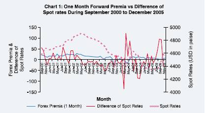
means market is expecting a steady appreciation of Indian rupee vis-à-vis
US dollar irrespective of the positive forward premia and in spite of higher
domestic interest rate in Indian market as compared with US market. Further, the
relationship with spot exchange rate and forward premia in Indian market is found
to be very weak. This means future spot rate of US dollar vis-à-vis
Indian rupee is driven by some other factors in addition to forward premia.
Based on equations (1), (2) and (3) above with µ=0 (i.e. assuming rational
expectation) for the period September 2000 to December 2005, the regression equation
in Indian context takes the following form | St+δt-
St = 0.00005 - 0.0583* (ft - St) | =
(0.028) (- 0.102) |
R2 = 0.0002;
t-statistic are give in parenthesis.
Question then arises is what does
forward premia in Indian forex market represent and what factors are accounted
for by the market players while determining the forward premia itself. The paper
endeavoured to analyse these factors in Section II in general and in section III
in respect of Indian forex market in particular. Section
II Forward Market for foreign exchange is extremely
important particularly for importers and exporters. This is so because international
trade results in exposure in foreign currencies. Forward Market helps the traders
in hedging the risks of this inevitable exposure in foreign currency. On the other
side there are players in foreign exchange market who offer the forward rates
for the foreign currency. A well-developed market helps in getting the better
rates for the traders promoting international trade and consequently the general
economic development.
Offering forward rates for any commodity always
involve trying to forecast the future price of the commodity keeping in view the
opportunity cost. It may require knowledge about how the price of the underlying
product is determined in the market. One also needs to be aware about the factors
influencing the price of the product. Countries are free to decide the type of
exchange rate arrangements, which could be described to vary in different degrees
from fixed to flexible exchange rate. It is practically impossible to strictly
follow either a completely fixed or flexible exchange rate. International Monetary
Fund publishes an annual report listing the different regimes followed by its
member countries. There are many countries that are following ‘pegged exchange
rate’ mechanism whereby their domestic currencies are fully pegged with
some other major foreign currency like USD. Forecasting the exchange rate and
thereby working out the forward rates for currencies following different regimes
would be different.
From the perspective of the economists there are three
classes of explanatory variables, viz., price level, interest rates and
the balance of payments to explain the behaviour of the exchange rate. The Purchasing
Price Parity or PPP hypothesis tries to explain how the price levels affect the
exchange rates. It says the relative exchange rate S = kP/P*, where P is
the price level in the domestic economy, P* is that in the other country and k
is a constant parameter. Taking differences after taking logarithms gives us Δs=
Δp - Δp* giving us the idea
how the forward rates could be influenced by the change in the level of prices
in the two economies. However, it is noted that over a short or medium term, PPP
hypothesis is conclusively rejected.
Though, it cannot
be said that the price levels have no impact on exchange rate movement or the
forward rates.
In the earlier section the paper has already talked about the
influence of interest rates on the exchange rates. Both the major Interest Rate
Parity hypotheses, i.e., Covered Interest Rate Parity (CIP) and Uncovered
Interest Rate Parity (UIP) have drawn lot of attention of the researchers, but
UIP is more interesting in the context of this paper because it involves the variable,
expected future spot rate, unlike CIP.
That the trade imbalances would
have a bearing on the behaviour of exchange rates has been recognised very early.
However, the earliest models to relate the current account to the exchange rate
followed the Marshallian tradition of treating the exchange rate as a relative
price to clear the market with the “elasticities approach”. The limitations
of this approach led to the emergence of “absorption approach” in
the 1950s. Among the series of subsequent models, the Mundell– Fleming model
is most referred. The Mundell-Fleming Model adds a balance of payments equilibrium
condition to the IS-LM Model. This extends the closed economy IS-LM framework
to examine the interplay between monetary policy and exchange rate policy. In
particular, the model emphasises the differences between fixed and floating exchange
rates. It is very apparent that the forward rate is supposed
to be arrived at from the expectations on the future exchange rates, which is
expected to get influenced by the sets of variables mentioned above as well as
all of the “news”. This news could indicate change in the economic
conditions or even political stability. The price of the crude oil in the international
market is found to impact the forex market. The forward premia is particularly
sensitive to any news having financial bearing and reacts or over-reacts instantly.
Coming back to the Indian context where the exchange rate regime currently followed
is largely market determined, the intervention by the regulator may also
play important role at least over short to medium term. Over the years, internationally,
the central banks are found to intervene through the Forward Market in Conjunction
with the spot market for making larger impact. In the next section the paper looks
at the behaviour of forward premia on US dollar vis-à-vis Indian
rupee. Section III
As
observed in Section I, UIP hypothesis does not hold good for the Indian market,
as the slope coefficient is significantly different from one. Furthermore, there
are other factors, which also influence the forward market in India. This section
has tried to identify the factors that affect forward premia in Indian forex market,
i.e., “What drives forward premia in Indian forex market?” - Is
it inflation-differential?
- Is it interest-rate differential?
- Is
it FII flows?
- Is it the current account balance in BoP?
To answer this question, an attempt is made to carry -out some exploratory exercise
based on Forward Premia - annualized (INR vis-à-vis US$), Inflation
differential between Indian and US economy (i.e. WPI for India* –
CPI for US economy) (Chart 2), Interest Rate differential between 91 Day Treasury
Bills in India and US (Chart 3); Interest Rate differential between MIBOR - one
month and LIBOR-one month (Chart 4), FIIs inflows and Current Account Balance
(Chart 5). Chart 2 indicates that forward premia has a weak relationship
with Inflation-differential in US and Indian Economy.
Chart 3 indicates
the relationship between 3 months forward premia (annualised) and interest rate
differential in Government of India and the US T Bills is also not strong,
though there is good co-movement some of the time. Hence the variable is considered
for further analysis.

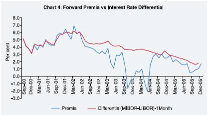
Chart
4 indicates that relationship between forward premia - 1 month (annualised) and
interest rate differential between one month MIBOR and 1 month LIBOR, is stronger
than the above two. However, there are other factors (supply
side as well as demand side), viz., fresh flows by Foreign Institutional
Investors (FIIs) and current account balances play important roles in determining
the forward premia as can be seen from the respective regression equation and
its analysis given below. In Chart 5 below the premia is shown with the 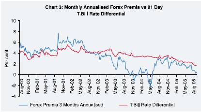
current
account balance (USD 100 million) and FII net investment (in USD 100 million).
Performing the regression of one month Forward Premia for USD vis-à-vis
INR (Annualised) vs Inflation Differential, Interest Rate Differential
(one month MIBOR – one month LIBOR), FII Portfolio Investment (net flows)
and India’s current account balance (CAB) over the entire period Septemer
2000 to September 2005, it is observed that the coefficient for Inflation differential
is not statistically significant, thereby prompting us to drop from final analysis.
Since, the information 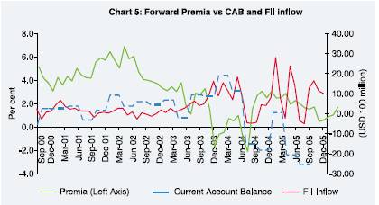
on current account balances is available to the market with a lag, introduction
of lagged value of current account balance (1 quarter lag) showed improvement.
Furthermore, balance of payments (BoP) current account quarterly balance is distributed
equally for intervening months for regression analysis, due to non-availability
of monthly CAB data. In this connection, instead of CAB, trade balance data, which
is available on monthly frequency was also tried, but did not show good result.
Equation:
Forward Premia (Y) = f (Interest rate differential (IRD),
Current Account Balance –lagged (CAB), FIIs Net flows (FIINF))
(Period : September
2000 to September 2005) | | Coefficients | Standard
Error | t Stat | P-value |
Intercept | -2.3166 | 0.5822 | -3.9788 | 0.0002* |
IRD | 1.4393 | 0.1316 | 10.9339 | 0.0000* |
CAB | -0.1039 | 0.0145 | -7.1897 | 0.0000* |
FIINF | -0.0917 | 0.0212 | -4.3220 | 0.0001* |
* : Siginificant at 5 per cent. |
Regression
Statistics | R
Square | 0.7695 |
Adjusted R Square | 0.7574 |
Standard Error | 0.9870 |
Durbin-Watson D | 1.084 |
Furthermore to check the influence of RBI intervention
on forward premia, RBI’s Intervention (Net Purchase of USD) has also been
tried as regressor and it was found that the variable is not statistically significant
indicating that RBI intervention in forex market does not make significant impact
in determination of forward premia and it only helps in smoothing the volatility
in forex premia. Similarly 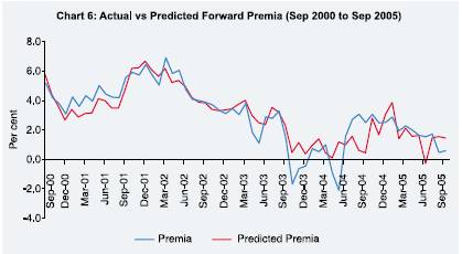
inclusion of Trade Balance as regressor in place of Current Account Balance
has not resulted in improvements. Though the regression
above shows a reasonable fit with expected signs, in the actual and estimated
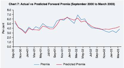
premia plot in Chart 6 some change in pattern is observed over the period. This
motivated breaking the period of observation into two parts, i.e., September
2000 to March 2003 and April 2003 to September 2005 and explores the behaviour
separately. For the September 2000 to March 2003 period, the regression
gives the following result:
| Coefficients | Standard
Error | t
Stat | P-value |
Intercept | -1.3441 | 0.5754 | -2.3357 | 0.0272 |
IRD | 1.2402 | 0.1164 | 10.6567 | 0.0000* |
CAB | -0.0610 | 0.0198 | -3.0746 | 0.0048* |
FIINF | -0.0076 | 0.0452 | -0.1678 | 0.8680* |
* : Siginificant
at 5 per cent |
Regression
Statistics | R
Square | 0.8135 |
Adjusted R Square | 0.7928 |
Standard Error | 0.4800 |
Durbin - Watson D | 0.980 |
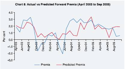
For the period April 2003 to September 2005 period, the regression gives
the following result:
| Coefficients | StandardError | t
Stat | P-value |
Intercept | -0.5304 | 1.3627 | -0.3892 | 0.7003 |
IRD | 0.7686 | 0.4251 | 1.8081 | 0.0822* |
CAB | -0.0842 | 0.0240 | -3.5074 | 0.0017* |
FIINF | -0.0682 | 0.0309 | -2.2041 | 0.0366* |
* : Siginificant at 5 per cent |
Regression
Statistics | R
Square | 0.3324 |
Adjusted R Square | 0.2554 |
Standard Error | 1.2429 |
Durbin - Watson D | 1.121 |
As observed there is a marked difference in the regression results in the two
periods. Also, the Durbin Watson D statistics, for the regression run for the
full study period, indicates the possible presence of first order autocorrelation.
One way to deal with the autocorrelation is to include the lagged value of the
dependent variable as a regressor. However, it is felt that the past forward premia
might have less influence on the current forward premia compared to the observed
change in the exchange rate in the immediately preceding period. It was indeed
found out that introducing the lagged forward premia was not improving the regression.
Therefore, another variable AOCER : Annualised observed change in exchange rate
of USD vis-à-vis INR was introduced. This variable captures the immediate
trend in the exchange rate. Further, this also goes well with self-fulfilling
nature as observed during the times of volatility in any financial market. The
regression results based on the four variables for the period of October 2000
to September 2005 are as follows:
| Coefficients | Standard
Error | t
Stat | P-value |
Intercept | -2.0894 | 0.5210 | -4.0107 | 0.0002* |
IRD | 1.3955 | 0.1186 | 11.7658 | 0.0000* |
CAB | -0.1109 | 0.0130 | -8.5095 | 0.0000* |
FIINF | -0.0889 | 0.0187 | -4.7451 | 0.0000* |
AOCER | 0.0477 | 0.0113 | 4.2146 | 0.0001* |
* : Siginificant at 5 per cent. |
Regression
Statistics | R
Square | 0.8236 |
Adjusted R Square | 0.8108 |
Standard Error | 0.8702 |
Durbin-Watson D | 1.144 |
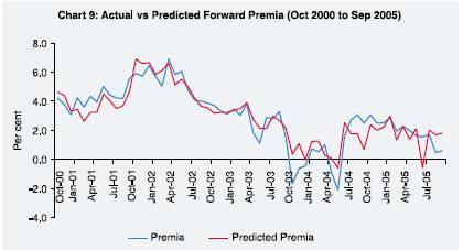
It
is observed that the incorporation of the exchange rate variable, i.e, AOCER has
improved the fitness in terms of the Adjusted R Square (0.75 to 0.81) and other
parameters. More importantly, it is observed that the fit is good uniformly and
in particular much better in the second half of the study period, which experienced
volatile movements in forward premia. It is also observed that the first order
autocorrelation has come down though its presence cannot still be ruled out. This
leaves further scope for exploratory analysis in this area especially in respect
of Indian forex market, which is still emerging. Section
IV
Conclusion
In
Section I, we have seen that the UIP hypothesis does not hold good for Indian
market. It has been explored that individually no single factor is able to explain
the behaviour of the forex premia in Indian forex market. From the analysis carried
out above, we could see that in specific time window one of the factors may have
dominated in determining the movement of the forex premia. The paper has also
explored the movement of the forex premia by dividing the study period in two
parts and observed that in the first part (September 2000 to March 2003) of the
study period the coefficient of the interest rate differential was much higher
than the second part (April 2003 to September 2005). The role of foreign institutional
investment in driving the forward premia is observed to be more dominant in second
part than the first. This vindicates the perception that the premia is more and
more being influenced by demand and supply factors rather than the interest rate
differential in recent times. Though these two variables along with the interest
rate differentials were able to explain the behavior of the premia in the first
part of the study period, the relationships have weakened considerably in recent
times.
In a longer time horizon, differential between
interest rates (i.e. LIBOR-MIBOR differential) together with foreign institutional
investment in Indian market, current account balance and the change in the observed
Exchange rate are largely able to explain the behaviour of the forex premia in
Indian forex market. The findings suggest that forex premia of US$ vis-à-vis
Indian rupee is driven to a large extent by the interest rate differential in
the inter bank market of the two economies coupled with capital receipts and excess
of current accounts payments on accounts of imports in relation to exports as
well as the change in the exchange rate of USD vis-à-vis Indian
rupees.
Table
1 : Currency distribution of reported foreign exchange market turnover1 |
Percentage
shares of average daily turnover in April | Currency | 1989 | 1992 | 1995 | 1998 | 2001 | 2004 |
US dollar | 90 | 82.0 | 83.3 | 87.3 | 90.3 | 88.7 |
Euro | . | . | . | . | 37.6 | 37.2 |
Deutsche mark2 | 27 | 39.6 | 36.1 | 30.1 | . | . |
French franc | 2 | 3.8 | 7.9 | 5.1 | . | . |
ECU and other EMS currencies | 4 | 11.8 | 15.7 | 17.3 | . | . |
Japanese yen | 27 | 23.4 | 24.1 | 20.2 | 22.7 | 20.3 |
Pound sterling | 15 | 13.6 | 9.4 | 11.0 | 13.2 | 16.9 |
Swiss franc | 10 | 8.4 | 7.3 | 7.1 | 6.1 | 6.1 |
Australian dollar | 2 | 2.5 | 2.7 | 3.1 | 4.2 | 5.5 |
Canadian dollar | 1 | 3.3 | 3.4 | 3.6 | 4.5 | 4.2 |
Swedish krona3 | … | 1.3 | 0.6 | 0.4 | 2.6 | 2.3 |
Hong Kong dollar3 | … | 1.1 | 0.9 | 1.3 | 2.3 | 1.9 |
Norwegian krone3 | … | 0.3 | 0.2 | 0.4 | 1.5 | 1.4 |
Korean won3 | … | … | … | 0.2 | 0.8 | 1.2 |
Mexican peso3 | … | … | … | 0.6 | 0.9 | 1.1 |
New Zealand dollar3 | … | 0.2 | 0.2 | 0.3 | 0.6 | 1.0 |
Singapore dollar3 | … | 0.3 | 0.3 | 1.2 | 1.1 | 1.0 |
Danish krone3 | … | 0.5 | 0.6 | 0.4 | 1.2 | 0.9 |
South African rand3 | … | 0.3 | 0.2 | 0.5 | 1.0 | 0.8 |
Polish zloty3 | … | … | … | 0.1 | 0.5 | 0.4 |
Taiwan dollar3 | … | … | … | 0.1 | 0.3 | 0.4 |
Indian rupee3 | … | … | … | 0.1 | 0.2 | 0.3 |
Brazilian real3 | … | … | … | 0.4 | 0.4 | 0.2 |
Czech koruna3 | … | … | … | 0.3 | 0.2 | 0.2 |
Thai baht3 | … | … | … | 0.2 | 0.2 | 0.2 |
Hungarian forint3 | … | … | … | 0.0 | 0.0 | 0.2 |
Russian rouble3 | … | … | … | 0.3 | 0.4 | 0.7 |
Chilean peso3 | … | … | … | 0.1 | 0.2 | 0.1 |
Malaysian ringgit3 | … | … | … | 0.0 | 0.1 | 0.1 |
Other currencies | 22 | 7.7 | 7.1 | 8.2 | 6.5 | 6.1 |
All currencies | 200 | 200.0 | 200.0 | 200.0 | 200.0 | 200.0 |
1 Because two currencies
are involved in each transaction, the sum of the percentage shares of individual
currencies
totals 200% instead of 100%. The figures relate to reported “net-net”
turnover, i.e., they are adjusted for both
local and cross-border
double-counting, except for 1989 data, which are available only on a “gross-gross”
basis.
2 Data for April 1989 exclude domestic trading involving the Deutsche
mark in Germany.
3 For 1992-98, the data cover local home currency trading
only.
Source : Triennial Central Bank Survey 2004,
BIS |
Table
2 : Reserve Bank’s Sale and Purchase of USD (in Million) |
Month | Sales
in US Dollar | Purchase
in US Dollar | Net
in US Dollar | 2000:09
(SEP) | 1,015.1 | 728.0 | -287.1 |
2000:10 (OCT) | 1,004.5 | 510.5 | -494.0 |
2000:11 (NOV) | 4,392.5 | 8,078.6 | 3,686.1 |
2000:12 (DEC) | 2,204.5 | 2,049.4 | -155.1 |
2001:01 (JAN) | 1,334.7 | 2,166.3 | 831.6 |
2001:02 (FEB) | 456.5 | 1,080.4 | 623.9 |
2001:03 (MAR) | 1,138.7 | 1,745.0 | 606.3 |
2001:04 (APR) | 1,626.8 | 1,608.5 | -18.3 |
2001:05 (MAY) | 613.5 | 1,082.3 | 468.8 |
2001:06 (JUN) | 1,169.2 | 1,205.5 | 36.3 |
2001:07 (JUL) | 1,130.7 | 859.0 | -271.7 |
2001:08 (AUG) | 1,052.0 | 1,733.8 | 681.8 |
2001:09 (SEP) | 2,326.1 | 1,432.0 | -894.1 |
2001:10 (OCT) | 1,043.4 | 1,280.8 | 237.3 |
2001:11 (NOV) | 1,435.0 | 2,977.1 | 1,542.1 |
2001:12 (DEC) | 1,341.2 | 2,381.6 | 1,040.4 |
2002:01 (JAN) | 1,390.5 | 2,781.7 | 1,391.2 |
2002:02 (FEB) | 1,202.5 | 1,769.3 | 566.8 |
2002:03 (MAR) | 1,428.0 | 3,710.6 | 2,282.5 |
2002:04 (APR) | 1,605.5 | 2,082.0 | 476.5 |
2002:05 (MAY) | 1,146.5 | 1,232.5 | 86.0 |
2002:06 (JUN) | 571.3 | 812.0 | 240.8 |
2002:07 (JUL) | 685.0 | 2,514.1 | 1,829.1 |
2002:08 (AUG) | 1,459.0 | 2,637.8 | 1,178.8 |
2002:09 (SEP) | 1,956.4 | 2,921.5 | 965.1 |
2002:10 (OCT) | 1,422.5 | 2,593.5 | 1,171.0 |
2002:11 (NOV) | 972.0 | 3,086.5 | 2,114.5 |
2002:12 (DEC) | 1,551.5 | 3,230.5 | 1,679.0 |
2003:01 (JAN) | 1,046.0 | 2,830.5 | 1,784.5 |
2003:02 (FEB) | 1,171.0 | 3,505.5 | 2,334.5 |
2003:03 (MAR) | 1,339.1 | 3,188.5 | 1,849.4 |
2003:04 (APR) | 1,511.0 | 2,942.5 | 1,431.5 |
2003:05 (MAY) | 1,636.0 | 3,978.0 | 2,342.0 |
2003:06 (JUN) | 982.1 | 1,878.5 | 896.4 |
2003:07 (JUL) | 2,950.0 | 6,095.5 | 3,145.5 |
2003:08 (AUG) | 1,360.0 | 3,711.5 | 2,351.5 |
2003:09 (SEP) | 4,229.4 | 6,574.0 | 2,344.6 |
2003:10 (OCT) | 5,227.7 | 6,821.0 | 1,593.3 |
2003:11 (NOV) | 580.0 | 4,029.0 | 3,449.0 |
2003:12 (DEC) | 484.4 | 3,372.5 | 2,888.1 |
2004:01 (JAN) | 1,028.0 | 4,321.5 | 3,293.5 |
2004:02 (FEB) | 2,163.0 | 5,519.5 | 3,356.5 |
2004:03 (MAR) | 2,789.0 | 6,170.5 | 3,381.5 |
2004:04 (APR) | 3,332.9 | 10,758.5 | 7,426.5 |
2004:05 (MAY) | 3,439.5 | 3,219.5 | -220.0 |
2004:06 (JUN) | 1,383.0 | 969.5 | -413.5 |
2004:07 (JUL) | 1,179.5 | | -1,179.5 |
2004:08 (AUG) | 880.5 | 5.0 | -875.5 |
2004:09 (SEP) | 124.0 | 143.0 | 19.0 |
2004:10 (OCT) | 104.0 | 5.0 | -99.0 |
2004:11 (NOV) | | 3,791.5 | 3,791.5 |
2004:12 (DEC) | 108.2 | 1,501.5 | 1,393.3 |
2005:01 (JAN) | | | 0 |
2005:02 (FEB) | | 4,974.0 | 4,974.0 |
2005:03 (MAR) | | 6,030.0 | 6,030.0 |
2005:04 (APR) | | | 0 |
2005:05 (MAY) | | | 0 |
2005:06 (JUN) | 103.6 | | -103.6 |
2005:07 (JUL) | | 2,473.0 | 2,473.0 |
2005:08 (AUG) | 451.0 | 2,003.0 | 1,552.0 |
2005:09 (SEP) | | | 0 |
2005:10 (OCT) | | | 0 |
Source
: Reserve Bank of India Bulletin. | References
Baillie, R.T., R. E. Lippens, and P. C. McMahon (1983): “Testing Rational
Expectations and Efficiency in the Foreign Exchange Market”,
Econometrica,
51, 553-564
Bekaert, G. and R. Hodrick (2001): “Expectations Hypotheses
Tests”, Journal of Finance, 56, 4, 1357-1393.
Cochrane, J.
(2001): Asset Pricing, Princeton, N.J., Princeton University Press.
Database on Indian Economy (https://cdbmsi.reservebank.org.in/)
Fama E. (1984):
“Forward and Spot Exchange Rates”, Journal of Monetary Economics,
14, 319-338.
Flood, R.P and A. K. Rose (2002): “Uncovered Interest Parity
in Crisis”, IMF Staff Papers, 49, 2, 252-266.
Frenkel, J. A.
(1977): “The Forward Exchange Rate, Expectations, and the Demand for Money:
The German Hyperinflation”, American Economic Review, 67, 653-670.
Geweke, J. and E. Feige (1979): “Some Joint Tests of the Efficiency of Markets
for Forward Foreign Exchange”, Review of Economic Statistics, 61,
334-341.
Hakkio, C. S. (1981): “Expectations and the Forward Exchange
Rate”,
International Economic Review, 22, 663-678.
Hansen
L.P. and R. Hodrick (1980): “Forward Exchange Rates as Optimal Predictors
of Future Spot “Rates: An Econometric Analysis”, Journal of Political
Economy, 88, 5, 829-853.
Hansen L.P. and R. Hodrick (1983): “Risk
Averse Speculation in the Forward Foreign Exchange Market: An Econometric Analysis
of Linear Models” in Exchange Rates and International Macroeconomics,
ed. by J.A. Frenkel. Chicago: University of Chicago Press for National Bureau
of Economic Research, 1983.
Hodrick, R. (1987): The empirical evidence on
the efficiency of forward and futures foreign exchange markets, Harwood Academic
Publishers, Chur, Switzerland Horvath M.T.K and M. W. Watson (1995): “Testing
for Cointegration When Some of the Cointegrating Vectors are Prespecified”,
Econometric Theory, 11, 5, pp. 952-984.
Lewis K. (1989): “Changing
Beliefs and Systematic Rational Forecast Errors with Evidence from Foreign Exchange”,
American Economic Review, 79, 621-36.
Mark N.C. and Y. Wu (1998):
“Rethinking Deviations from Uncovered Interest Rate Parity: The Role of
Covariance Risk and Noise”, Economic Journal, 108, 1686-706.
Phillips P.C. B. (1991): “Error Correction and Long Run Equilibrium in Continuous
Time”, Econometrica, 59, 967-980.
RBI (2005): Annual Report,
2004-05.
Triennial Central Bank Survey of Foreign Exchange and Derivatives
Market Activity by Bank for International Settlements (BIS), 2004.
Wang P.
and T. Jones (2002): “Testing for Efficiency and Rationality in Foreign
Exchange Markets - A Review of the Literature and Research on Foreign Exchange
Market Efficiency and Rationality with Comments”,
Journal of International
Money and Finance, 21, 223-239.
* Shri Anil Kumar Sharma
is Director and Shri Anujit Mitra is Assistant Adviser in Operational Analysis
Division of Department of Statistical Analysis & Computer Services (DESACS). The
authors wish to thank Dr. Balwant Singh, Adviser, DESACS for his comments on the
earlier version of the paper. An earlier version of the paper was also presented
at the Eighth Money and Finance Conference at Indira Gandhi Development Research
Institute (IGIDR) in March 2006. The views expressed in the paper are of the authors
own and do not reflect the views of the organization to which they belong. *In
the case of India, a representative CPI is not available at present. |
 IST,
IST,


