This article highlights that rural and urban inflation in India exhibit similar dynamics – in terms of trend, cycle, persistence and volatility – notwithstanding sporadic divergences which do not last long. Empirical findings on the presence of a long run cointegrating relationship between them, a statistically significant error correction process restoring alignment, and convergence across states validate the relevance of the inflation target as the nominal anchor at the national level for both rural and urban areas as well as all states.

Introduction

In a very diverse country like India, characterised by a large share of rural population (68.8 per cent as per Census 2011) and high dependence on agriculture and allied activities for livelihoods (57.8 per cent of rural workers in usual status as per Periodic Labour Force Survey 2018-19), it becomes imperative to examine the behavior of rural and urban inflation to understand their implications for policy making. Ignoring the regional dimensions of inflation may limit the effectiveness of a single monetary policy in adequately meeting the requirements of all regions equally (Weber and Beck, 2005; Weyerstrass et al. 2011) and may make inferences about economic outcomes misleading (Brandt and Holz, 2006).

Large and persistent divergence between rural and urban inflation could result in differences in real wage rates, real interest rates and inflation expectations which can pose challenges for monetary policy. From an operational perspective, such divergence, if persists, can further complicate generating reliable model-based forecast of inflation, which acts as the intermediate target of monetary policy under the flexible inflation targeting (FIT) framework. Against this backdrop, examining the dynamics of rural and urban inflation - in terms of their trend, drivers, volatility, persistence and convergence - to understand their implications for monetary policy is the main motivation of this article.

The remainder of the article is organised as follows. Section II presents an analysis of rural and urban inflation to understand the nature and pattern of inflation diversity/convergence. Section III reviews select literature on regional inflation divergence to draw inferences on their relevance to and implications for monetary policy. The co-movement of rural and urban inflation at the aggregate (all-India) level along with the nature of convergence of state level rural and urban inflation is tested in Section IV. Section V sets out the concluding observations.

II. Stylised Facts

Headline CPI inflation¹ witnessed significant and sustained moderation during 2012-13 to 2018-19, before rising thereafter. Both rural and urban inflation exhibited a similar trend with the only difference that urban inflation started rising from 2018-19. Moreover, annual average urban inflation which was ruling below rural inflation till 2017-18, moved above it during 2018-19 and 2019-20 (Chart 1a). Both food and non-food inflation contributed to the divergence between urban and rural inflation (Chart 1b).

Contributions of major groups to annual inflation, however, mask intra-year movements in inflation in the rural and urban areas, given significant differences in the composition of the CPI baskets. It can be observed from monthly data that rural and urban all groups inflation have often diverged during 2012-2020, but the divergence has not persisted long, suggesting the existence of a long-run relationship between them (Chart 2a). This is further corroborated by the fact that the divergence has been driven not by any single component over time but by different components of CPI – food, fuel and excluding food and fuel items – during different periods. For instance, the observed divergence between rural and urban inflation during 2018-2019 period largely mirrored the divergence in food inflation reflecting supply shocks (Chart 2b), while the divergence during 2015-2016 period was caused by excluding food and fuel inflation (Chart 2c). On the other hand, fuel inflation exhibits occasional large differences between rural and urban areas, reflecting the differences in the consumption pattern, increasingly market-linked pricing of fossil fuels and subdued price pressures in traditional fuel items like firewood and chips and dung cakes in rural areas (Chart 2d). In 2020-21 so far, headline inflation has firmed up further reflecting the impact of COVID-19 induced lockdown measures and associated supply chain disruptions. Rural and urban inflation, however, have displayed significant convergence, broadly mirroring the trends in food price inflation after April-May 2020. This could be attributed to the nature of the spread of COVID-19 and imposition of various lockdown measures to contain the spread, which was initially confined to urban areas before eventually spreading to rural areas.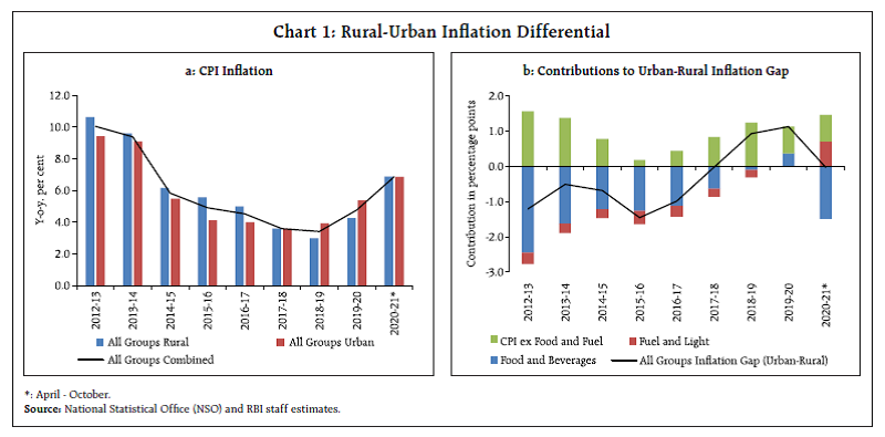

A deeper investigation into the food inflation dynamics reveals that generally urban food price inflation turns out to be higher than rural food price inflation during periods of upswings in food prices, while the opposite happens during downswings. This phenomenon is observed in both vegetables (perishables) and other food items, i.e., food ex-vegetables. Such asymmetric behavior could partly be explained by supply chain disruptions like floods, unseasonal rainfall or transporters’ strikes that make transportation of food items sourced from rural areas to urban areas difficult, which in turn lead to opportunistic pricing and hence higher urban food price inflation. However, as the supply situation normalises and the easing cycle starts, urban price fall faster as urban sellers seek to liquidate their stocks.

In the case of fuel group, after remaining high till 2018-19, rural fuel inflation started easing significantly thereafter owing to penetration of clean fuel like liquefied petroleum gas (LPG) [due to Pradhan Mantri Ujjwala Yojana (PMUY)] and electricity [due to Deen Dayal Upadhyaya Gram Jyoti Yojana (DDUGJY) and Pradhan Mantri Sahaj Bijli Har Ghar Yojana – Saubhagya], which eased price pressure in items like firewood and chips. In ex-food and fuel category, the gap between rural and urban inflation has narrowed significantly in last three years, driven mainly by clothing and footwear, health, personal care and effects, and household goods and services. Penetration of various government funded health schemes [such as Ayushman Bharat Pradhan Mantri Jan Arogya Yojana (AB-PMJAY) and other state level health insurance schemes] in rural areas would also have contributed in narrowing the gap.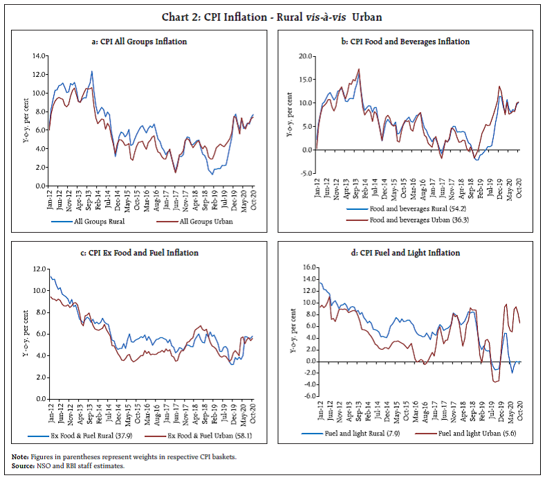

Thus, while different components have driven the divergence between rural and urban inflation in different episodes, the divergence has not persisted unidirectionally over time. As the comparison of inflation between rural and urban areas is based on the two price indices (and not raw prices), it is important to note that part of the divergence may arise from the way the price indices are constructed, i.e., because of the differences in coverage, sampling, price collection mechanism, and weights of items/sub-groups/groups in respective CPI baskets. For instance, the food group has higher weight in rural CPI (54.2 per cent) than urban CPI (36.3 per cent), while there is no housing component in rural CPI (Table 1). Another important difference was in the price collection mechanism - with National Statistical Office (NSO) collecting prices in urban areas and post offices doing the same for rural areas until October 2018, when NSO was assigned this job for both rural and urban CPI.

Even after adjusting for housing to make rural and urban inflation more comparable, annual average CPI urban inflation is found to have remained below rural all through up to 2017-18; and higher since 2019-20 (Chart 3).

An analysis of key summary statistics reveals that rural and urban inflation behave similar to CPI-C (headline) inflation, particularly in terms of mean and volatility (as measured by the standard deviation of monthly y-o-y inflation) (Table 2). The mean and volatility of food inflation in the two areas are even closer.

Sub national policy changes as well as asymmetric impact of national policy changes can also cause divergence in regional inflation. Policy changes in China played an important role in determining the price index differences between rural and urban areas for a certain period (Zhang Xuechun, 2010). In India, policy interventions in the form of tax, subsidies, agricultural marketing reforms and penetration of targeted welfare schemes would have also contributed to regional price differences, primarily due to asymmetric impact depending on the coverage/ access. In fact, there was a marked downward shift in overall inflation and major groups’ inflation in rural and urban areas during 2016-2020, albeit with some differences, which coincided with the adoption of FIT framework in India (Chart 4).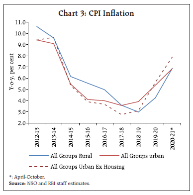

At the sub-groups level, rural inflation was higher than urban inflation prior to the adoption of FIT for most of the components. Post FIT, inflation in the subgroups seem to be clustered around 4 per cent, indicating a general reduction in inflation dispersion across the components, excluding a few such as perishables like fruits and vegetables, and pulses (Chart 5).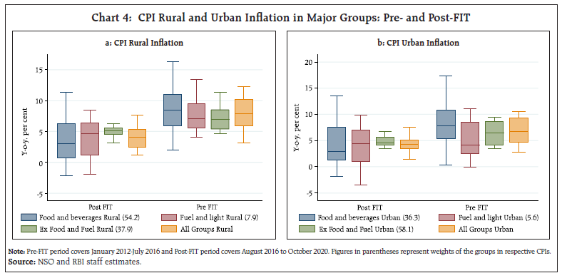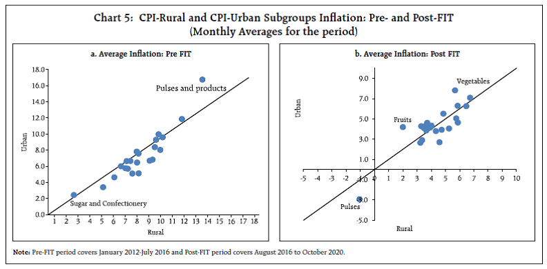

The marked shift in inflation was accompanied by moderation in inflation persistence or backward-looking price setting behavior, for both rural and urban areas until 2018, albeit with some differences (Chart 6.a). Subsequently, inflation persistence increased in both rural and urban areas on shocks to food prices from unseasonal and excessive rains impacting crops and supply disruptions, before falling² again with the gradual normalisation of supply chains. A decomposition of headline inflation into trend and cycle reveals similar behavior in trend inflation in both urban and rural areas, albeit with a relatively early reversal of declining trend in urban inflation compared to rural inflation (Chart 6.b). It is, however, interesting to note that the cyclical components in both rural and urban inflation have largely behaved similarly.

III. Literature Review

Inflation dynamics at the regional level gained particular significance in the literature after the adoption of the Euro in the Euro-area (Weber and Beck, 2005 and Beck et al., 2009). Regional price dynamics in other major economies like the USA has also been analysed to draw relevant lessons for the euro-area-wide average inflation target based on Harmonized Index of Consumer Prices (HICP) (Cecchetti et al., 2002). Given that, a single target for the entire country/ common currency area (CCA) makes sense only when inflation rates in different countries in the CCA/regions of an economy are not very different from each-other, policy makers often devote attention to the reasons behind inflation differences. Inflation differentials could represent rigidities in the economy, translating into loss of competitiveness (Alberola, 2000) and could also have a potentially destabilising asymmetric effect due to differences in real interest rates (Beck et al., 2009). A number of studies have investigated the reasons for the observed inflation differentials (Hendrikx and Chapple, 2002; ECB, 2003; ECB, 2005). Some of the reasons for divergence in inflation rates among European Union countries include differential impact of exchange rate movements (Honohan and Lane, 2003, 2004), inflation persistence (Angeloni and Ehrmann, 2004) and the role of supply shocks vis-à-vis demand shocks (Duarte and Wolman, 2002). Among emerging market economies (EMEs), a study for China highlights the role of policy changes, urban-rural retail sales of consumer goods, degree of urbanisation and fixed asset investment in explaining rural-urban price differences (Zhang Xuechun, 2010). Systematic differences in prices of goods and services across regions may imply differences in the costs of living; therefore, ignoring spatial price differences while explaining economic outcomes can be misleading (Brandt and Holz, 2006).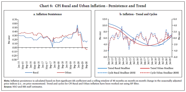

A related strand of literature has examined the mean reverting behavior and the overall cross-regional dispersion of inflation rates. Building on the work of Barro and Sala-i-Martin (1992), a study on inflation rates of individual regions of the European Union reveals fall in inflation dispersion during certain time period and significant mean reverting behavior, albeit at a relatively modest rate (Weber and Beck, 2005). A slow rate of convergence in prices has also been documented for the US cities (Cecchetti et al., 2002). Along similar lines, a study for China using cointegration and error correction technique concluded that rural price level converges to the urban price level (Zhang Xuechun, 2010). An investigation into the compliance with the Law of One Price (LOP) across six regions of Argentina for the period 2016-2019 suggests the existence of convergence in prices and cointegration across regions (González, 2020).

In the case of India, majority of the literature has focused on the factors that influence regional inflation dynamics, which include transportation costs, natural endowments of the states, restrictions on factor mobility, region-specific consumption items, inflation persistence, expenditure and tax policies of state governments, per capita income growth and other supply side and structural factors (Das and Bhattacharya, 2008; Jha and Dhal, 2019; Patnaik, 2016). On higher observed rural inflation than urban inflation, Bhandari and Srinivas (2015) concluded that structural bottlenecks are not letting rural Indians benefit fully from global disinflation. Inflation differential among the states could also be explained by convergence of prices and the subsequent inflation catch-up occurring at the state level (Patnaik, 2016). Notwithstanding observed wide dispersion in inflation across states driven by food price inflation, state level inflation tends to converge to the national inflation over time, underpinning the choice of national level CPI inflation as the nominal anchor for monetary policy in India (Kundu et al., 2018).

IV. Co-integration and Convergence

Given the close co-movement between rural and urban inflation (at the all-India level) over time, an empirical exercise is conducted in a single equation framework using fully modified ordinary least squares (FMOLS) (Phillips and Hansen, 1990) on monthly inflation data for January 2012-October 2020 to test the existence of a long-run equilibrium relationship between the two. As both rural and urban inflation series were found to be non-stationary at level but with same order of integration [i.e., I(1)], the following single equation cointegrating regression (i.e., long run equation) was estimated using FMOLS:

where DUM2013 (May-August 2013=1, ‘0’ otherwise) is introduced to capture the taper tantrum impact and temporary aberration in the direction of divergence between rural and urban inflation, while DUM2018 (October 2018 to October 2019=1, ‘0’ otherwise) is introduced to account for the shift in the data collection system for rural CPI, from post offices to the NSO field staff, in October 2018.

In the next step, similar to widely used Engle- Granger (1987) two-step approach (Gerrard and Godfrey, 1998), the one period-lagged equilibrium error (û_t-1) from eq.(1) was used for estimating the error correction mechanism (ECM) using OLS as:

where ∆ is the difference operator and β2 is the coefficient of the error correction term. A negative and significant β2 captures the speed of adjustment towards the long-run equilibrium.

The Engle-Granger tau-statistic and z-statistic from the estimated eq.(1) confirm presence of a long-run cointegrating relationship between rural and urban inflation (Table 3). Moreover, the coefficient of error correction term in eq.(2) [β2 = (-) 0.12] was also found to be statistically significant with the expected negative sign, suggesting that 12 per cent of the previous period’s disequilibrium³ (i.e., the deviation between the actual and long-run) is corrected every month. The residual diagnostics tests suggest absence of serial correlation and heteroscedasticity indicating robustness of the estimates. The stability of the parameter estimates is also validated by the cumulative sum of squares (CUSUM) test (Chart 7).

Since all-India rural and urban CPI are compiled as a weighted sum of state level rural and urban price indices, it is interesting to examine the behaviour of rural and urban inflation at the state level. The state-level mean rural and urban inflation differentials with respect to all India rural and urban inflation, respectively, have fallen over time implying convergence of state wise rural (urban) inflation to all India rural (urban) inflation (Chart 8.a). Rural and urban inflation seems to be converging across states as evident from the more or less symmetric nature of the estimated kernel density plot of the state wise annual average differential between urban and rural inflation during 2012-13 to 2019-20 (Chart 8.b). The inflation spread moves in a wide range and the distribution is also leptokurtic implying differing extent of ruralurban linkages.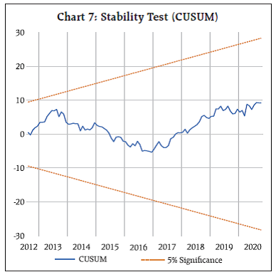

The variability of rural and urban inflation across states from the national average shows the absence of any particular trend, suggesting relative stability in the relationship between rural and urban inflation across states (Chart 9). The prevailing regional dispersion of inflation thus does not undermine inferences and analysis based on national level inflation metric.

Against this backdrop, a formal test of convergence between urban and rural inflation across states was conducted in a random effects panel regression model for the period 2012-13 to 2019-20 taking 35⁴ states and union territories (UTs). Drawing from the literature (Weber and Beck, 2005), β convergence, which allows identification of the speed of unconditional convergence was tested by estimating the following equation: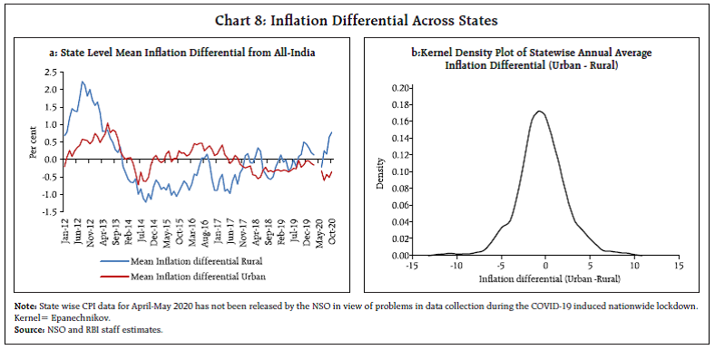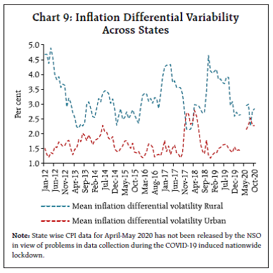

Where, ∆ is the difference operator, i represents states, πi_ut and πi_rt are state wise urban and rural annual average inflation, respectively, and ϵ_it is the error term. A negative sign of β⁵ signifies existence of convergence and its (absolute) size reflects the speed of convergence. In other words, negative sign of β would imply that states with an initial relatively high urban-rural inflation gap would experience increase in inflation more slowly (or decrease in inflation faster) in the subsequent period than states with an initial relatively low urban-rural inflation gap. Thus, the existing urban-rural inflation rate gap across states would diminish. The results of our analysis confirm existence of β convergence, i.e., convergence of rural urban inflation across states and that any shocks to inflation at the state level dissipates at a reasonable speed (Table 4). The Breusch-Pagan Lagrange Multiplier (LM) test suggests that an OLS regression is better suited than a random effects panel regression and, therefore, the OLS results are also reported as a robustness check (Table 5).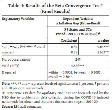

The empirically observed co-movement of rural and urban inflation at the aggregate level as well as convergence at the state level suggests that one inflation rate at the national level captures the overall inflation dynamics in India well.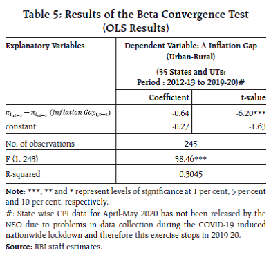

V. Conclusion

Rural urban inflation dynamics in India reveals close co-movement, with episodic divergences driven by different components – food, fuel or ex-food and fuel – which do not persist long. Both trend and cyclical components are found to be similar for urban and rural inflation. Gradual decline in inflation persistence in the pre COVID-19 period (up to 2018) was also observed for rural and urban inflation.

Empirical estimates reveal that the observed differentials between rural and urban inflation are transient and both exhibit a long-run equilibrium relationship, with a significant error correction in the short-run. At the state level also urban and rural inflation rates converge over time. These findings support the relevance of one inflation target as the nominal anchor at the national level for both rural and urban areas as well as all states.

References

Alberola Ila, E. (2000), “Interpreting Inflation Differentials in the Euro Area”, Economic Bulletin/ Banco de España, April, pp. 61-70.

Angeloni, I. and M. Ehrmann (2004), “Euro Area Inflation Differentials”, European Central Bank, Working Paper Series No. 388.

Barro, Robert. J. and Xavier Sala-i-Martin (1992), “Convergence”, Journal of Political Economy, 100(2), pp. 223-251.

Beck, Guenter W., Kirstin Hubrich and Massimiliano Marcellino (2009), “Regional Inflation Dynamics Within and Across Euro Area Countries and a Comparison with the United States”, Economic Policy, January, pp. 141–184.

Brandt, Loren and Carsten A. Holz (2006) “Spatial Price Differences in China: Estimates and Implications”, Economic Development and Cultural Change, University of Chicago Press, vol. 55(1), October, pp. 43-86.

Cecchetti, S. G, N. C. Mark, and R. J. Sonora (2002), “Price Index Convergence among United States Cities”, International Economic Review, 43(4) November, pp. 1081-1099.

Das, Praggya and Asish Thomas George (2017), “Comparison of Consumer and Wholesale Price Indices in India: An Analysis of Properties and Sources of Divergence”, RBI Working Paper Series No. 05, March.

Das, S. and K. Bhattacharya (2008), “Price Convergence across Regions in India”, Empirical Economics, 34(2), pp. 299-313.

Duarte, M. and A. L. Wolman (2002), “Regional Inflation in a Currency Union: Fiscal Policy vs. Fundamentals”, European Central Bank Working Paper Series 180.

Engle, Robert F. and W. J. Granger (1987), “Co- Integration and Error Correction: Representation, Estimation, and Testing”, Econometrica, Vol. 55, No. 2, March, pp. 251-276.

European Central Bank (ECB) (2003), “Inflation Differentials in the Euro Area: Potential Causes and Policy Implications”, Monetary Policy Committee of the European System of Central Banks, September 2003.

European Central Bank (ECB) (2005), “Monetary Policy and Inflation Differentials in a Heterogeneous Currency Area”, European Central Bank Monthly Bulletin, May, pp. 61–77.

Gerrard, W. J. and L.G. Godfrey (1998), “Diagnostic Checks for Single Equation Error Correction and Autoregressive Distributed Lag Models”, The Manchester School, Vol.66, No.2, March, pp. 222-237.

Gonzalez, Fernando. A. I. (2020), “Regional Price Dynamics in Argentina (2016–2019)”, Regional Statistics, Vol. 10. No. 2. pp. 83–94; DOI: 10.15196/ RS100205.

Hendrikx, M. and B. Chapple (2002), “Regional Inflation Divergence in the Context of EMU”, MEB Series (discontinued) 2002-19, Netherlands Central Bank, Monetary and Economic Policy Department.

Honohan, P. and P. R. Lane (2003), “Divergent Inflation Rates in EMU”, Economic Policy, 18(37), pp. 357-394.

Honohan, P. and P. R. Lane (2004), “Exchange Rates and Inflation under EMU: An Update”, The Institute for International Integration Studies Discussion Paper Series No. 31.

Jha, Arvind and Sarat Chandra Dhal (2019), “Spatial Inflation Dynamics in India: An Empirical Perspective”, Reserve Bank of India Occasional Papers, Vol. 40, No. 1.

Kundu, Sujata, Vimal Kishore and Binod B. Bhoi (2018) “Regional Inflation Dynamics in India”, RBI Monthly Bulletin, November.

Patnaik, Anuradha (2016), “Inflation Differential and Inflation Targeting in India”, Prajnan, Vol-XLV, No. 1.

Phillips, Peter C. B. and Bruce E. Hansen (1990), “Estimation and Inference in Models of Cointegration: A Simulation Study”, Advances in Econometrics, Vol 8, pages 225-248.

Weber, Axel A. and Guenter W. Beck (2005), “Price Stability, Inflation Convergence and Diversity in EMU: Does One Size Fit All?”, Centre for Financial Studies Working Paper No. 2005/30, November.

Weyerstrass, K., B. Aarle, M. Kappler and A. Seymen (2011), “Business Cycle Synchronisation within the Euro Area: In Search of a ‘Euro Effect’”, Open Economies Review, 22(3), pp. 427–446.

Zhang Xuechun (2010), “The Urban-Rural Differences of Inflation in China”, People’s Bank of China, January.

* This article is prepared by Binod B. Bhoi, Himani Shekhar and Ipsita Padhi, Department of Economic and Policy Research, Reserve Bank of India. The views expressed in this article are those of the authors and do not represent the views of the Reserve Bank of India.

¹ In India, headline inflation is measured by the year-on-year per cent change in the all-India Consumer Price Index-Combined (CPI-C) series with base year 2012=100 released by the National Statistical Office (NSO), Ministry of Statistics and Programme Implementation (MOSPI), Government of India and it has been used to define the inflation target under the flexible inflation targeting (FIT) framework since August 2016. The CPI-C, in turn, is constructed following a bottom-up approach by first compiling price index at the item level and then at the sub-group/group level for both rural and urban areas across states, which are then combined using respective fixed weights.

² The AR coefficients for the recent period i.e. May-October 2020 are not significant at 5 per cent level of significance especially for urban inflation.

³ Adjustment to long run equilibrium was found to be bidirectional.

⁴ Arunachal Pradesh is not considered as CPI urban is not published on a regular basis for this state.

⁵ As pointed in Weber and Beck, 2005; it may be noted that - unlike in the growth literature - the reported measures for the adjustment speed lack a sound theoretical foundation. Still, they can give some idea on how fast convergence occurs.

⁶ A random effects generalized least squares regression was carried out. The choice between random effects and fixed effects panel estimation was based on the Hausman test.