Press Release

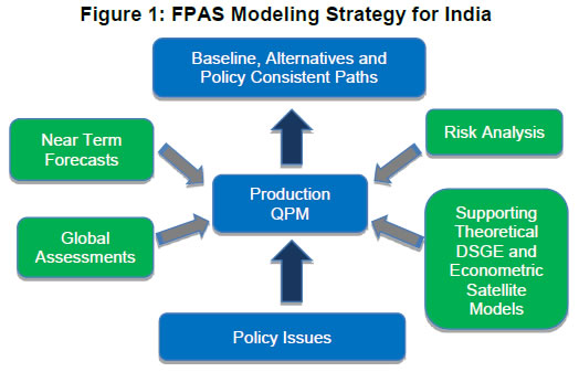
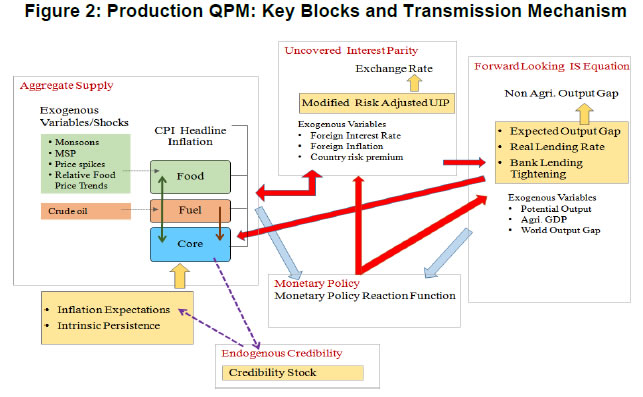
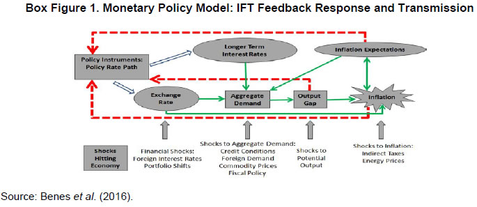
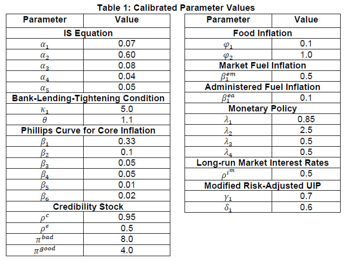
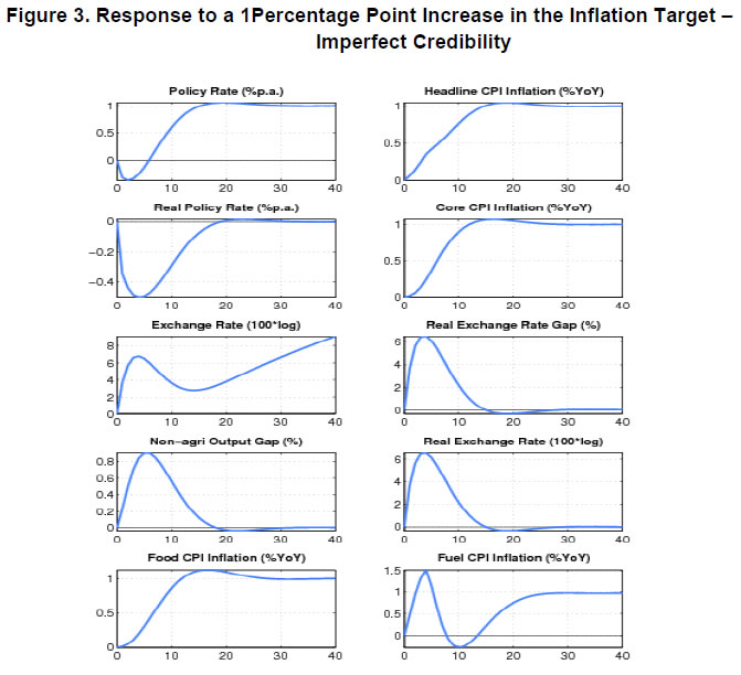
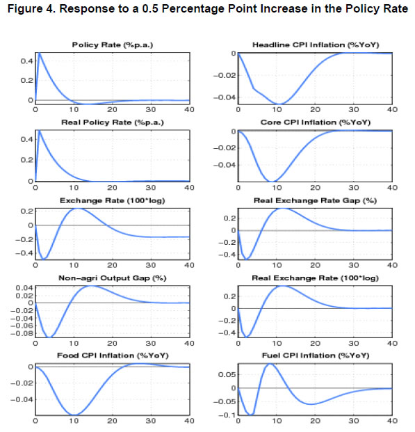
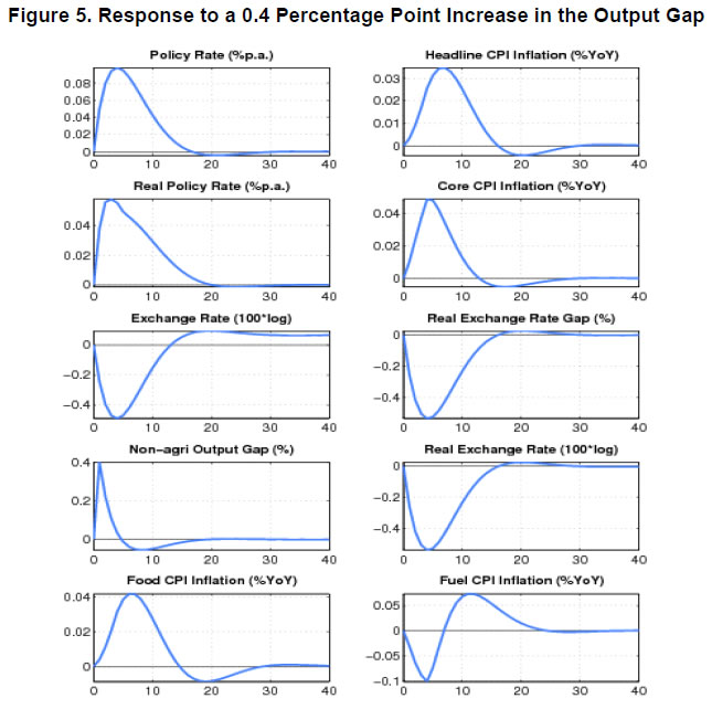
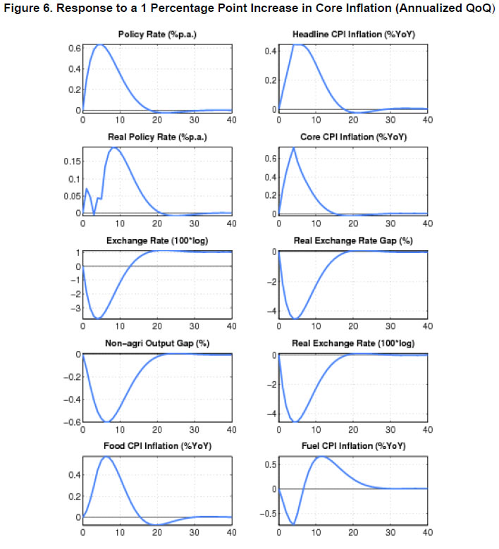
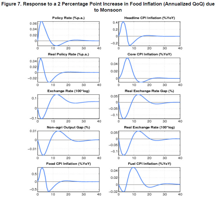
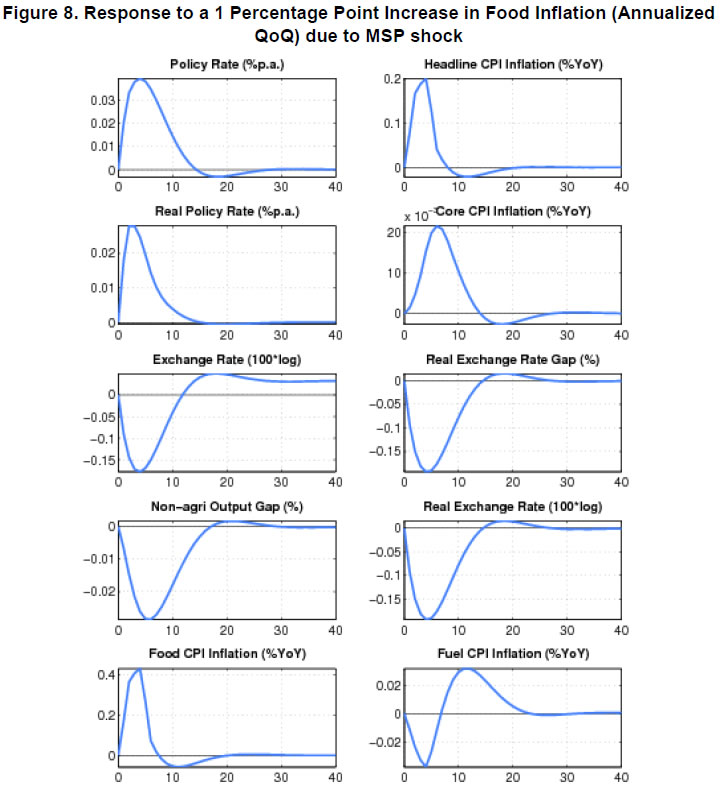
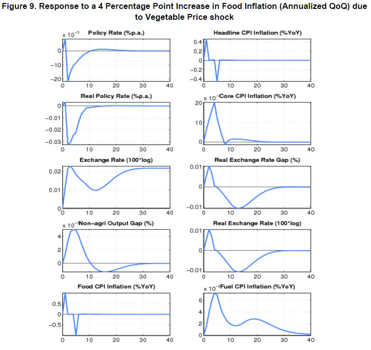
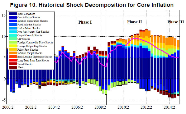
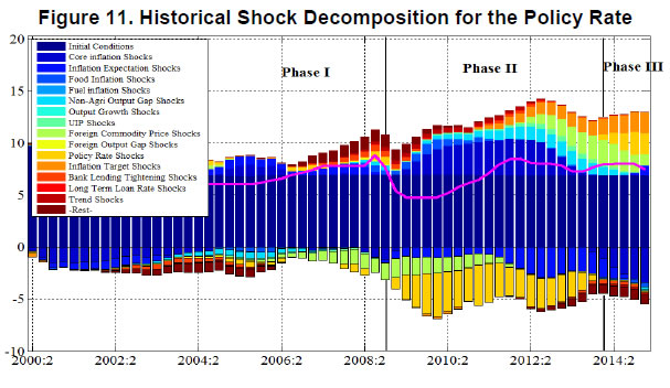
RBI Working Paper Series No. 08
Quarterly Projection Model for India: Key Elements and Properties
^@Jaromir Benes, Kevin Clinton, Asish Thomas George, Pranav Gupta, Joice John,
Ondra Kamenik, Douglas Laxton, Pratik Mitra, G.V. Nadhanael, Rafael Portillo,
Hou Wang and Fan Zhang

Abstract

¹This paper outlines the key features of the production version of the quarterly projection model (QPM), which is a forward looking open economy gap model, calibrated to represent the Indian case, for generating forecasts and risk assessment as well as conducting policy analysis. QPM incorporates several India specific features like the importance of the agricultural sector and food prices in the inflation process; features of monetary policy transmission and implications of an endogenous credibility process for monetary policy formulation. The paper also describes key properties and historical decompositions of some important macroeconomic variables.

JEL Classification: E5, Z0

Keywords: forecasting, economic projections, macroeconomic models

I. Introduction

Based on the recommendations of the Report of Expert Committee to Revise and Strengthen the Monetary Policy Framework (January 2014), the subsequent Agreement on Monetary Policy Framework signed by the Government of India (GoI) and the Reserve Bank of India (RBI) on February 20, 2015² and through the amendment of the Reserve Bank of India Act in May 2016³, the RBI has formally adopted a Flexible Inflation Targeting (FIT) framework. The FIT framework is also known as inflation forecast targeting (IFT) wherein the medium term inflation projections become the intermediate target for policy. Since there are lags in the monetary policy transmission and trade-offs between meeting an inflation target and stabilizing output growth, the successful implementation of IFT requires reliable medium-term forecasts and some knowledge of how policy actions will affect the goal variables of inflation and output. The main policy instrument which is in practice is the policy repo rate, and it has its impact on output and inflation through a complex transmission mechanism involving longer term interest rates, exchange rate, credit and expectations of households and markets among others. Hence, a regime of inflation targeting relies on forecasts and policy analysis that adequately take into account relevant India-specific linkages. In such a scenario macroeconomic models aid the policymakers to assemble their understanding of the economy and structure their thinking, discussions and forecasting exercise. It provides a systematic framework to characterize and analyze risks around any conditional baseline projection path of key macro variables and their policy implications. The fundamental role for monetary policy in this framework is to provide an anchor for inflation and inflation expectations. Under FIT in order to anchor expectations around the desired outcome, communication with the public on the rationale of the monetary policy stance becomes imperative. A small, coherent, and sensible economic model could also play a role of the useful vehicle for this sort of communication.

The purpose of this paper is to propose a model based Forecasting and Policy Analysis System (FPAS) to provide support for inflation forecast targeting (Berg, et. al. 2006a,b). In many of the central banks that have adopted FIT, a suite of models is used to arrive at an assessment of the medium term path of the economy (Black et al., 1994; Black et al. 1997; Coats, Laxton, and Rose, 2003). FPAS has a quarterly projection model (QPM), which is a forward looking open economy calibrated gap model that helps to generate a medium term policy path consistent with meeting the targets/mandate set under the FIT regime. The QPM serves as a device to organize thoughts and data coherently in the form of a baseline assessment, balance of risk to the baseline projections and the nature of policy response to various kinds of shocks (Berg, et al. 2006a). The QPM is augmented by a number of satellite models which provide insights into the trends in real variables and sectoral dynamics. The objective of this paper is to sketch out such a model with India specific features to capture the dynamics relevant to an emerging market economy. These include, inter alia, a disaggregated analysis of inflation (food, fuel and core) with a specific focus on food inflation dynamics and the dampened nature of impacts of interest rate movement on exchange rate, among others. The broad structure of FPAS is discussed in Section II. Section III describes the key elements of QPM. The important equations in QPM and its calibrations are explained in Section IV and V respectively. Section VI illustrates the model properties through impulse response functions. The historical decompositions are narrated in Section VII. Concluding remarks are presented in Section VIII.

II. Suite of Models in FPAS

The FPAS is a framework for assimilating macroeconomic information relevant to monetary policy decision making process, consistent with a theoretical framework. The FPAS uses a suite of models to achieve its objective. First among these is the QPM, which is used to produce the baseline forecasts and alternative scenarios for the outlook. A key feature of the main model is an endogenous policy interest rate, which responds to movements in the inflation rate and other variables, in a way to bring inflation back to the announced target over the medium term. This is an essential requirement under FIT, as pre-set path for the interest rate (including one implied by the current market yield curve) is not compatible with a nominal anchor. By ensuring that over time the rate of inflation and expectations of inflation converge to the target, the endogenous interest rate maintains the nominal anchor in the model.

From the operational perspective, it is desirable to have two different but closely linked versions of the QPM. The first one is core-QPM which is smaller, and can readily incorporate nonlinearities. This is important for realistic modeling of policy reaction functions, because policymakers would have high aversion to outcomes that approach dark corners in which conventional policy instruments lose effectiveness (Blanchard, 2014). For example, in major advanced economies, the main dark corner to be avoided in recent period relates to deflation and the zero lower bound on interest rates. Under circumstances where inflation and the policy interest rate are both near zero, and there is substantial excess capacity in the economy, policymakers would react much more strongly against yet another disinflationary shock than they would in a situation where the starting levels for inflation and the interest rate are well above zero, and output close to its potential level. In other times, destabilized inflation expectations have posed a threat in the opposite direction, and policymakers have reacted with a hard tightening of the screws (e.g. the Volcker disinflation in the United States, 1979-83). A quadratic policy loss function capturing central bank’s behavior in setting policy interest rate better captures this kind of risk aversion than a linear rule. The Phillips curve is another relationship in which nonlinearity may be important, in view of the widespread evidence of flattening of the curve at wide negative output gap (high levels of unemployment). Both types of nonlinearities have been accommodated within core-QPM (see Benes et al., 2016 for details).

The second version, production-QPM is used for the production of baseline and alternative forecasts and risk assessment. On account of practical considerations, it contains a large number of variables and provides disaggregated details at sectoral level that is of interest to policymakers. An advantage is that it allows tractable derivation of underlying equilibrium trends for variables such as potential output, the real interest rate, and the real exchange rate. This, however, limits the menu of options for policy reaction functions and for the Phillips curve. The ensuing discussion is devoted to explain the structure and properties of the production-QPM.

Incorporating India-specific features to the FPAS remains the most challenging task⁴. For example the large share of food in total consumption and the predominance of agriculture sector in employment make it more likely that the developments in the price of food often play a major role in determining the trajectory of the headline inflation rate. This is reflected in the structure of production QPM, which can be used to simulate various types of shocks affecting the food sector, e.g. low monsoon rains, or a change in minimum support prices by the government.

Another important challenge is how to incorporate informed judgment as an important factor in forecasts and policy analysis. This is especially the case for short-term forecasts, which are made by sectoral experts, whose knowledge of current conditions and reliable short-run indicators may result in a far greater short-term forecast accuracy than that of purely model based forecasts. The experts may rely on a variety of models for their inputs—e.g. leading indicator models, and VARs. While the short-term forecasting process may be eclectic, the output of the short-run forecasts must have consistency with production-QPM, therefore, the short-run forecasts provides initial conditions for the medium-term forecast. In effect, production-QPM imposes macroeconomic consistency requirements on the short-term sectoral forecasts. The role of each type of model in the FPAS is sketched in Figure 1.

III. Production-QPM-Key Elements

As noted in the previous section, the production-QPM can be thought of as a system which includes representations of the steady state of the economy that establishes the long-term equilibrium conditions (Figure 2). Behavioral equations are represented in terms of deviations from steady state or gaps and the model depicts the path of the economy from the initial conditions to the equilibrium steady state.

The production-QPM is based on the principles of new-Keynesian open economy models, which embody the view that monetary policy matters for output dynamics in the short-run but, unlike their Keynesian predecessors, are built to a considerable extent on micro-foundations and rational expectations. This model is structured around the standard small open-economy model, with equations for output (the IS curve), inflation (the Phillips curve), the short-term interest rate (a policy reaction function), and the exchange rate (an uncovered interest parity condition). In the model, expectations at a given point in time are based on a combination of lagged outcomes, and model-predicted future outcomes. While during the short to medium term, expectations may show a bias, over the long run they converge to the outcomes predicted by the model. The production-QPM has a built-in endogenous process for evolution of monetary policy credibility over time, considering the fact that flexible inflation targeting has only been recently adopted as the monetary policy framework (Box 1). Within this structure, the production-QPM has tried to capture key India-specific sectoral details and dynamics; both in terms of inflation process–which include food and fuel price dynamics and their spillovers into core components and credibility driven inflation expectations augmented Phillips curve – as well as India specific characteristics of monetary policy transmission (Box 2).

Box 1: Monetary Policy Feedback

The credibility of the long-run inflation target underpins FIT (Laxton and N’Diaye, 2002; Goretti and Laxton, 2005). Everything pivots around the anchor provided by the firm expectations of the public that monetary policy will keep inflation stable and near the target rate in the long run (Levin, Natalucci, and Piger, 2004; Gurkaynak et al., 2007; Gurkaynak, Levin, and Swanson, 2010). This, in turn, requires that policy responds systematically to the requirements of this objective. The dynamic process underpinning the model is depicted in Box Figure 1.

With a forward-looking policy, when unanticipated disturbances hit the economy, in order to bring inflation back to the target, the future expected path of the policy interest rate is adjusted gradually over a period of time so as to limit disruptions to output. This policy feedback, via an endogenous short-term interest rate is represented by the red dashed arrows in the flowchart which ensures that the nominal anchor holds.

Expectations of future policy rate movements over the short term and medium term play a crucial role in the transmission mechanism, as depicted by the blue hollow arrows pointing at the ovals with “Longer Term Interest Rates” and “Exchange Rate”. The cost of borrowing of businesses and households is not the very short-term rate of interest directly controlled by the central bank. They borrow at longer terms. Policy rate affects these rates more through the impact of the policy rates expected in the future, and hence the whole yield curve. This is reflected in the rectangle for the “Policy Rate Path”—the whole path expected for the medium-term, not just the current setting.

The difference between FIT with an endogenous, forward-looking policy reaction function, and some other approaches to IT, for example use of an exogenous interest rate path (including a path derived from market forward rates), is that the latter two do not have explicit feedback from the expected future inflation rate to the policy instrument. If the model were modified to represent an exogenous interest rate path, the red dashed feedback arrows would be erased.

In situations where the actual rate of inflation differs from the long-run target, monetary policy would generally have to make a choice of appropriate response. The approach may be more or less rapid, depending on policymakers’ preferences regarding the short-run output-inflation trade-off. It might involve an asymptotic approach or a planned overshoot. Often out of the available options, the central bank will implement the one that “looks best,” i.e., the one that reflects its judgment as to the best outcome.

This applies to any gap between actual inflation and the long-run target. To provide a typical example, consider how the FIT would work following a sudden drop in the world price of oil. The Projection Team (PT) of the central bank would take into account its ramifications on all external variables, e.g., the level of demand in trading partners, and then, using the model, simulate the impact on the domestic economy. The baseline forecast, using the standard policy response of the model, would imply an interest rate path that, over the medium term, returns inflation to its long-run target rate, while taking into account the trade-off between the costs of inflation being away from target and the costs of output gap. Other policy responses might also be simulated to provide policymakers with a menu of options. In each case, there would be an entire time profile of short-term interest rates. The PT might also provide forecasts based on a couple of scenarios in which very different assumptions are used for the oil price, or, for that matter, other exogenous variables.

Box 2: Capturing India Specific Characteristics in Production QPM

Modeling for monetary policy in India faces challenges, but they are not unique in kind, or in order of difficulty, compared with the experience of a growing group of developing economies that has adopted inflation targeting as the basis for monetary policy. The QPM incorporates several frictions in order to reflect the characteristics of the Indian economy. This box provides three most important ones among them.

Monetary transmission mechanism (both through interest rates and exchange rates). Data shows that while the transmission from policy rates to money markets has been more or less complete, the transmission from the money market rates to the lending rates has been sluggish. In QPM, the persistence of the long-term market interest rates is calibrated to reflect this slow-moving feature. In addition, the model has built in Bank Lending Tightening (BLT) variable that captures the conditions in the credit market. On the exchange rate front, we consider a modified version of the risk-adjusted UIP condition that reduces the sensitivity of the exchange rate to domestic-foreign interest rate differentials. The weakened monetary policy transmission mechanism implies that the policy rate path needs to be adjusted more aggressively and highlights the need for measures that strengthen the monetary policy transmission mechanism to increase the effectiveness of monetary policy in the long run.

Various supply shocks to food prices. Food represents a large share of the Indian CPI (about 46 per cent), and swings in food prices tend to dominate medium-term fluctuations in the CPI. In the model, food inflation is driven mainly by three shocks, with differing impacts: monsoon shock, shock to government minimum support prices (MSPs) and shock to vegetable prices, e.g., onions. Monsoon shock has longer effects on inflation compared to vegetable price shock. A shock on vegetable prices raises food inflation sharply but then corrects itself with undershooting very rapidly due to the supply response and quick reaction of the government in terms of administrative actions and trade policies. A change in MSP of agriculture products can also affect food inflation. Given the lags in adjustment of prices, some carry-over of impact of hike in MSPs to few quarters of next year may be inevitable.

No established track record in providing a nominal anchor—until 2014 the RBI did not have an explicit overarching price stability mandate, and inflation expectations have not been well anchored. The history of moderate but unstable inflation doubtless weighs heavily in the public mind. This is captured in the QPM by a time-varying long-run inflation target, or equivalently, the perceived rate of inflation where inflation and inflation expectations converge. An insufficient monetary policy response to inflationary pressures could be rationalized in the model by a rising inflation target. In our calibration of the model, the inflation target is allowed to drift upwards gradually over time for the period 2009-2014.

IV. Key Equations in the Production QPM

This section presents the details of the key equations in the production QPM.

The Forward-Looking IS Equation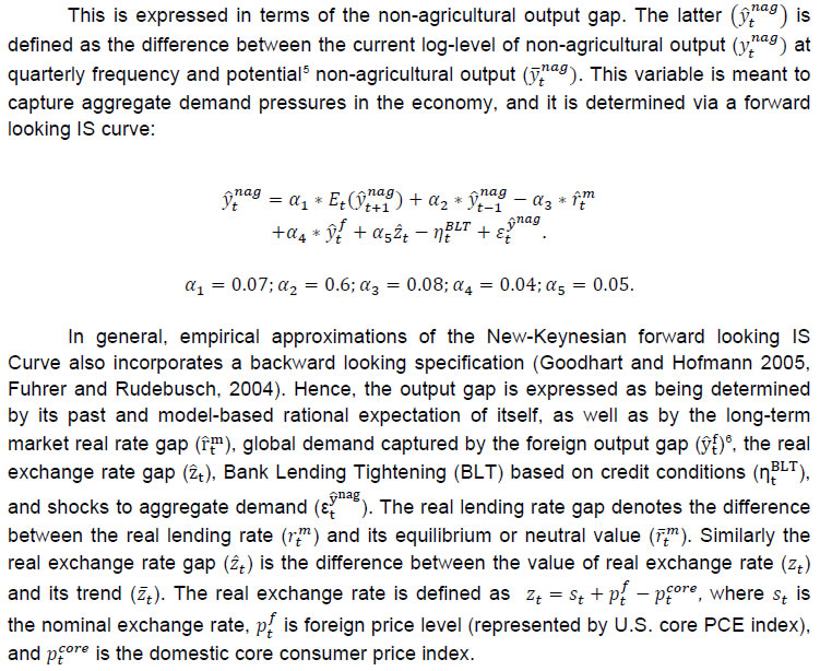

Calibration of FPAS like structures in most countries followed the approach of assigning a large coefficient value for lagged output; Berg et al. (2006b) suggest a range of 0.50 to 0.90 with lower value for countries with relatively large output gap volatility. Most studies in the emerging market context point to a dominant role of lagged output in output gap in the IS equation. In the Indian context, Patra and Kapur (2010) estimated the coefficient of lagged output to be at most 0.6 which inform our calibration of value at 0.6. This is also similar to the value used in Anand et al. (2014). The coefficient of lead output gap (α₁) is small (0.07) reflecting the need of acquiring confidence in promoting economic activity in India. Laxton and Scott (2000) suggest that for most of the economies the sum of coefficients of real interest rate and real exchange rate is relatively small as compared to the lag dependent variable. They report that for most economies the sum of coefficients would lie somewhere between 0.10 and 0.40. Empirical studies in the Indian case also find that the real interest rate coefficient in the IS equation is relatively small. For instance Patra and Kapur (2010) estimated it to be in the range 0.03 to 0.16. Taking these into consideration the real lending rate gap coefficient is taken to be 0.08. The coefficient of foreign output gap is calibrated using the export elasticities available from empirical studies and the share of exports in GDP. Similarly, α₅ is calibrated at 0.05 following the various empirical estimations in the Indian case, which under different specifications yield a coefficient in the range of 0.02 to 0.08 (see Patra and Kapur 2010). These calibrated coefficients are broadly in line with Anand et al. (2014).

Bank-Lending-Tightening Condition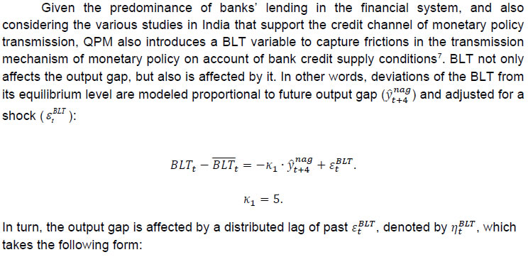

This weighting (with a peak effect at the 5 quarter lag) is intended to reflect a pattern in which an increase in Ɛ_t^BLT is expected to negatively affect spending by firms and households in a hump-shaped fashion, with an initial buildup and then a gradual rundown of the effects. If lending conditions are easier than might have been anticipated on the basis of expectations of future economic behavior, the effect will be a larger output gap and a stronger economy, also in a hump-shaped fashion. This reduced form for the effects of financial conditions on the real economy captures insights from structural models, e.g., Benes, et. al (2014a, b). The calibration of BLT equation largely follows Carabenciov et. al., (2008, 2013) which provide an illustration of how bank lending conditions are incorporated into a gap model (Global Projection Model, GPM). The historical decomposition in section VII validates the calibration as it largely reflects the observed trends in credit conditions during different periods in India.

The Phillips Curve for Core Inflation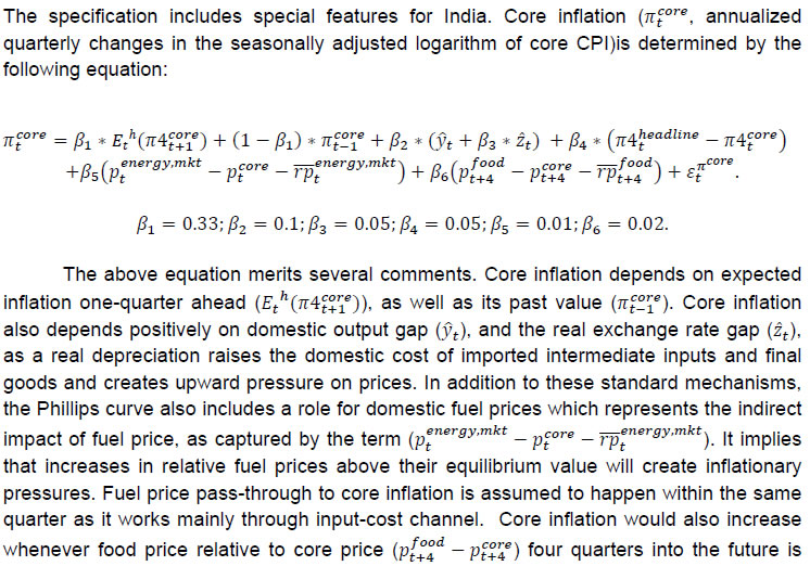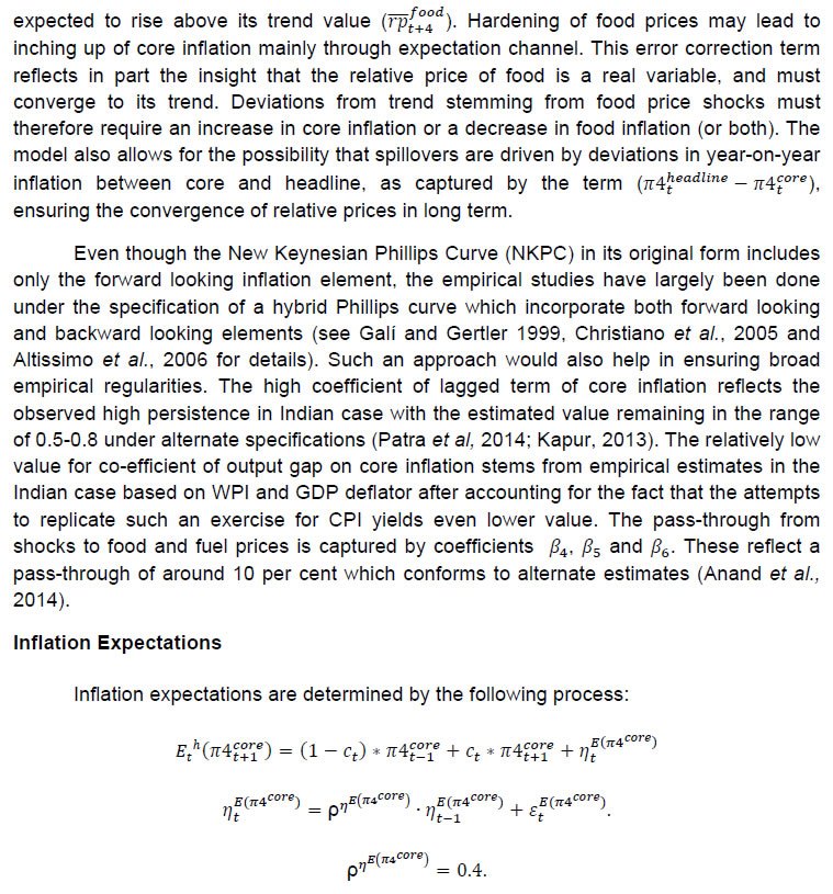

Inflation expectations are a weighted sum of one-quarter lagged year-on-year core inflation, and the model-based rational expectation of year-on-year inflation one quarter ahead⁸. The weights depend on the stock of policy credibility (C_t). C_t can range from 0 (no credibility), in which case expectations are completely backward looking, to 1 (perfect credibility), in which case inflation expectations are perfectly forward looking. The shocks in inflation expectations are assumed to be persistent and captured by the dynamics of the moving average term. For the purpose of historical decomposition, we have used a low credibility value of 0.25 to capture the absence of a nominal anchor and backward looking behavior of inflation expectations. Forecasting, however, is undertaken with an endogenous credibility specification which would capture the dynamic interaction between the central bank’s announced target, actual outcome and formation of inflation expectations.

Credibility Stock Building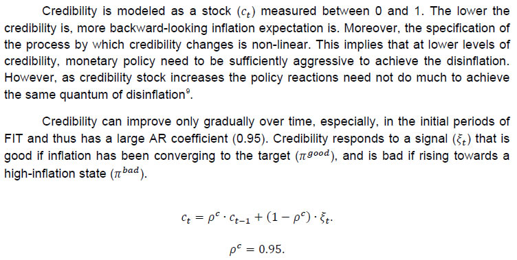

The credibility signal weighs the relative likelihood of inflation converging to the target versus being unanchored. It is higher if the current realized inflation is closer to the target. The error under the bad (good) regime is defined as the difference between the realized inflation and the expected inflation under the bad (good) regime. The expected inflation is a weighted average of the past observed inflation one quarter ago and the inflation target under the regime.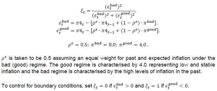

Food Inflation

The food inflation is characterized mainly through the dynamics of relative food price movements and shocks of different types. In the long run the food inflation is assumed to be equal to overall inflation, though it can diverge over different episodes. The dynamics of food inflation is modeled, as follows: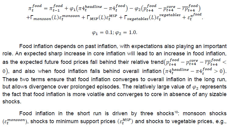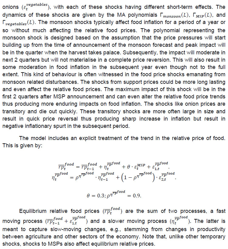

Energy Price Dynamics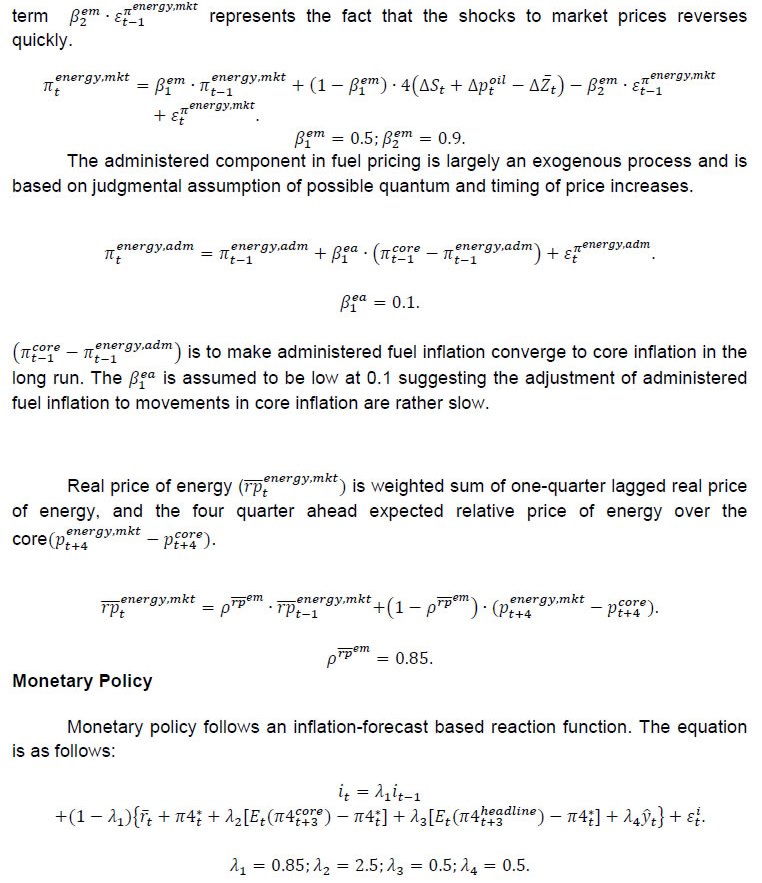

The original Taylor (1993) specification did not have an interest rate smoothing term. However, international experience suggests that central banks adjust their interest rate gradually, over a period of time, to change in economic conditions. Woodford (2003) also characterizes such response as optimal thus warranting the inclusion of an interest rate smoothing term in the monetary policy reaction function. Historically, studies on monetary policy in India have estimated large values for interest rate smoothing parameter. Calibrated and estimated monetary policy rules in a Taylor type framework have found values ranging from 0.7 to 0.9 for the smoothing parameter in various studies (Patra and Kapur, 2010, 2012 ; Bhattacharya and Patnaik, 2014; Anand et. al, 2014 ) which is broadly in line with 0.85 used in the production-QPM.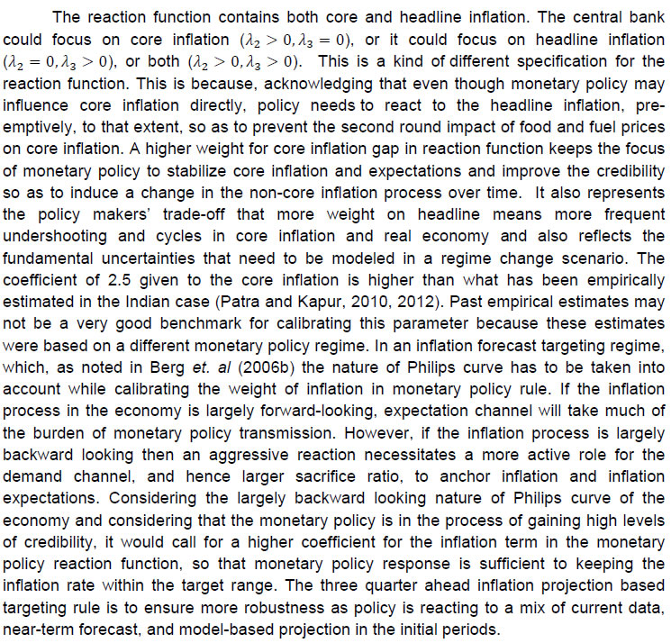

The steady-state perceived inflation target, or in other words, the long-run level that inflation will converge to, is set to the medium term inflation target. The unit root specification for inflation target allows creating long lasting impacts in inflationary process for changes in inflation target, the implications of which are illustrated in Section VI (1).

Long-run Market Interest Rates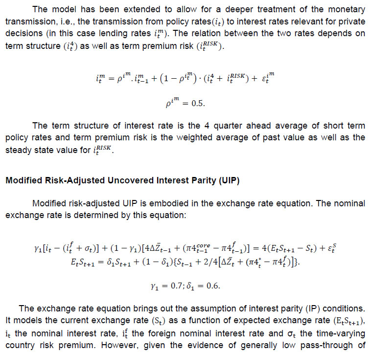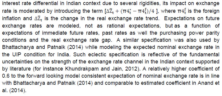

V. Calibration

Calibration of production-QPM is based on a wide variety of empirical evidence on the Indian economy, which are explained in the previous section, and the overall behavior of the economy in response to shocks, which are presented in the subsequent sections. The summary of the calibrated parameter values of the key equations are presented in Table 1.

It is important that simulation of the model as a whole produces results that are in line with the historical experience, and with standard macroeconomic theory. This means that a key criterion in the calibration of parameters is their combined effect on the overall properties of the model. In particular, one would want the model to replicate, to a fair approximation, broad empirical regularities observed historically in the response of the economy to shocks, or to changes in policy regime. In addition, policymakers and economists within the central bank would have, by virtue of years of experience, well-informed views of certain behavioral features of the economy. Credible forecasts and policy analyses take such views seriously into account. There is in any case a sound econometric rationale for calibrating to reflect the desirable system properties.¹¹ Traditional econometric estimation falls short of capturing high degree of simultaneity and forward looking aspect of the economy and assumes that the specification of the structure is known: the coefficients need to be estimated. Yet, in fact, the equations in models may be only a rough approximation to reality. Model builders deliberately avoid much of the detail, and many of the nonlinearities of the real world. This means that, a priori, conventional estimates of coefficients are unlikely to yield a useful multi-equation numerical structure, especially in view of the limitations on the data that are generally available—time series over periods free of structural breaks are usually quite short, relative to the needs of asymptotically consistent system estimation, especially in developing or emerging market economies.

Model solutions, simulations, forecasts and historical decompositions are carried out in IRIS toolbox in Matlab. In general, solving a model consists of three steps: (a) model needs to be linearised around a steady state, (b) forward-looking variables have to be solved, and (c) create a state-space representation. Steady states are computed using a nonlinear Newton-type algorithm. The simulations are based on a first-order approximate solution (calculated around steady state). Generalised Schur decomposition is used to integrate out the future expectations.

VI. Model Properties

The impulse-response functions corresponding to the unit standard deviation shocks are discussed in the following paragraphs. All the references to increases or decreases in any variable are relative to equilibrium levels.

(1) Inflation Target Shock—A Passive Policy Rate Change with Imperfect Credibility

This shock shows the implications of a change in the inflation target under conditions of a passive response of policy to inflation, and hence, of imperfect credibility (Figure 3). With the relevant increase in inflation expectations, the short-run decline in the real interest rate is greater than that in the nominal rate. Likewise, the short-run real depreciation of the currency, which is required by the uncovered interest parity condition, is greater than the nominal depreciation. The changes to the real interest rate and exchange rate raise demand for domestic output, opening a positive output gap for the non-agriculture sector. Over time, however, real variables return to their long-run equilibrium values—neutrality of money prevails. The nominal interest rate rises smoothly by an amount equal to the increased long-run inflation rate. During the period of adjustment, the real rate remains below the equilibrium real rate, which means that policy never actively resists inflation impulses —there is passive tolerance of the expected increase in inflation. The exchange rate overshoots for a while, before converging onto a long run rate of depreciation (due to positive inflation differential with the country of the foreign currency). The cumulative output gap until it returns to equilibrium is 2 per cent, implying a sacrifice ratio (cumulative increase in output per unit increase in equilibrium inflation rate) of approximately 2.

(2) Policy Rate Shock—Active Inflation Targeting Policy with Stable Inflation Expectations

An interest rate increase results in demand for domestic output to fall - a negative output gap opens up and induces an appreciation of nominal and real exchange rate (Figure 4). This reduces core and headline inflation. These effects are, however, only in the short run. Over time, to ensure a return to the inflation target, the central bank has to unwind the increase in the interest rate. The exchange rate goes through a cycle, and for a while it is above its long-run equilibrium value—the currency is temporarily undervalued. The stimulus that this provides to net exports creates a positive output gap for just long enough to neutralize the disinflationary effect of the initial interest rate increase. In the long run, the real exchange rate returns to its equilibrium value, which implies a nominal appreciation relative to the initial value, as the period of low inflation implies a permanently lower price level.

(3) Demand Shock

Monetary policy deals efficiently with demand shocks, as the effects on output and inflation go in the same direction (the “divine coincidence” of Blanchard and Gali, 2007). Thus, in Figure 5, a positive demand shock raises both the non-agriculture output gap and the rate of inflation (core rises by more than headline, as core prices are more sensitive to this output gap). Both the output gap and the deviation of inflation from target call for an increase in the real interest rate—i.e., a hike in the nominal rate greater than the rise in inflation. This causes an appreciation of the currency. These changes dampen demand, and over the medium term output returns to the potential level. With the elimination of excess demand, inflation goes back to the target rate. All real variables return to their original values, implying that the nominal exchange rate depreciates in line with the permanently increased price level entailed by the period of higher inflation.

(4) Cost Push Shock

A shock to the core inflation presents monetary policy with a difficult trade-off. The central bank has to raise the interest rate to ensure that inflation returns to target in the medium term, but this opens up a negative output gap (Figure 6). The nominal and real exchange rates appreciate. On unwinding of the interest rate as inflation falls to target, the output gap closes and output returns to the potential level.

(5) Monsoon Disappointment

A season of deficient monsoon is usually followed by fall in agriculture output and rise in agriculture prices. These inevitable effects will be anticipated in markets, with an immediate rise in inflation expectations for the year ahead. Moreover, empirically the after-effects of a poor monsoon have some duration (Figure 7). Policymakers, aiming to stabilize inflation expectations and to prevent the second round impact have to raise the interest rate. The exchange rate appreciates, and a negative output gap opens. However, with a return to normalcy in rains and harvests in the following year, the price spike will be followed by a price drop. This produces a cycle in food price inflation, and hence in the headline inflation rate and other macroeconomic variables.

(6) Agriculture Minimum Support Price Change

An increase in minimum support prices (MSP) raises food price inflation, and thus the headline inflation (Figure 8). Unlike the case of a poor monsoon, MSP increases have long lasting impact on food inflation as it affects the relative food prices. This necessitates a raise in the interest rate to anchor inflation expectations and to prevent the second round impact. Resultantly output gap opens up and exchange rate appreciates.

(7) Transitory Food Price Shock

A transitory food price shock could result from unexpected supply disruptions in certain commodities like vegetables due to unfavorable climatic conditions like unseasonal rains. Such a shock raises food price inflation more often quiet sharply. This effect is typically short-lived, as illustrated in Figure 9. Markets have a self-correcting tendency for disturbances of this kind, and the government has often acted to smooth the process of adjustment. As is indicated by the negligibly small movements in the figure, this kind of shock generally does not call for a monetary policy response of any significance.

VII. Historical Shock and Variable Decomposition

This section provides evidence of how well the production-QPM captures the dynamics within the historical data. The description and source of the data used for historical decomposition is described in Table 2.

The interpretations could be drawn from decomposing the historical data movements into various shocks in the model or by decomposing a variable into contributions of other variables. Two shock decompositions and two variable decompositions are discussed in this section. Even though the focus in this section is limited to 4 variables, the decomposition of changes can be applied to any endogenous variable in the model.

(1) Shock Decomposition – Policy Rate and Core Inflation

The first part in this section provides a break-up of the contributory factors to the evolution of core inflation and the policy interest rate in India since 2000 from the production-QPM. That is, it describes the model-simulated cumulative impact of the exogenous changes (shocks) on the two variables of interest i.e., inflation and policy rate. The interpretation of these results could be broadly described in three phases:

• Phase 1, 2000-08.Throughout much of this period inflation was low and steady (Figure 10) and the policy interest rate did not have to respond to large exogenous shocks. Towards the end of this phase monetary policy had to contend with a scenario of an oil price shock and strong domestic demand conditions.

• Phase 2, 2009-13. Large exogenous shocks from oil and food prices coupled with strong domestic demand resulted in persistently high inflation rates. In effect, the policy interest rate was generally too low to dampen the inflation impulses. In Figure 10 this is shown by the positive contribution to inflation emanating from policy rate shocks. And Figure 11 shows that the negative interest rate shocks—in effect, deviations from the inflation-forecast based monetary policy rule—were large for almost the entire duration of Phase 2. As inflation rose, in the absence of a well-defined nominal anchor, the implicit policy objective of the central bank for inflation, as perceived by the public rose with it. Simulation (1), section VII, provides a hypothetical illustration of such case.

• Phase 3, 2014-present. The central bank adopted a regime of flexible inflation targeting. The policy rate has followed the inflation-forecast based rule quite closely—i.e., there have been no large interest rate shocks. Inflation did drop faster than expected because of falling commodity prices, especially crude oil. Going forward, the new regime should provide a firmer anchor for inflation expectations, but given the large weight of food in the CPI basket, and the high volatility of food prices, food price shocks will continue to have large impact on the rate of inflation. Simulations (5), (6) and (7), illustrate this point.

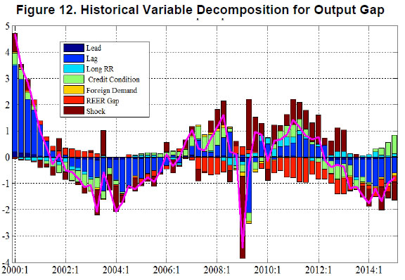
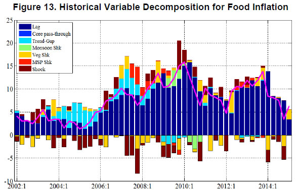
(2) Variable Decomposition – Output Gap And Food Inflation

In this part the evolution of output gap and food inflation in India is examined by decomposing them into contributions from various determinants. It describes the model-simulated impact of different factors on the two variables of interest i.e. output gap and food inflation.

The output gap which opened up sharply during the crisis period narrowed quickly and became positive supported by an accommodative monetary policy stance. The credit conditions then remained somewhat benign, even though an overvalued Rupee continued to hurt demand. Subsequently, credit conditions became tight on account of strict credit standards set out by banks leading to negative output gap. Post 2014 policy rate became accommodative helping output gap to move closer to zero. The large positive shocks to the aggregate demand during the period 2007-2012 could be attributed to various non-monetary measures like MGNREGA and other post crisis fiscal stimulus which provided a boost to aggregate demand during those periods (Figure 12).

The food inflation dynamics can be characterised by the relative food price trend and various shocks that affect food prices. The positive slope in the relative food price trend contributed to food inflation during 2004-2008.The large MSP increases contributed to food inflation in 2008 -09 and 2012. The deficient monsoon contributed to inflation in 2009. The large unexpected shocks in the form of onion price spikes affected food inflation many times but were transitory (Figure 13).

VIII. Conclusion

This paper outlines a coherent framework based on FPAS for generating forecasts and risk assessment as well as conducting policy analysis, which could be useful to policy makers in a FIT regime. Models, based on DSGE methodology, or traditional econometrics, may be used as satellite models to complement the FPAS. Results from these models may be used either in the parameterization of QPM, or to shape judgments about forecast assumptions and so on. Satellite models would also provide disaggregated sectoral dynamics and projections of key macro-variables considered in the QPM.

QPM incorporates key features of the Indian economy, such as:

• Importance of the agricultural sector and food prices in the inflation process;

• India specific monetary policy transmission;

• Building policy credibility and non-linearity.

Model simulations illustrate how the central bank might respond to demand and supply shocks to return inflation over the medium term to the announced target. The paper also provides an informative decomposition of the contributions of causal factors to the historical evolution of some of the key macroeconomic variables.

^@ The paper is the outcome of the technical collaboration between RBI and IMF to develop a quarterly projection model for India. The authors would like to express their sincere thanks to B.K Bhoi, Sitikantha Pattanaik, Muneesh Kapur, Rajesh Singh, Kenneth Kletzer, Rudrani Bhattacharya and anonymous referees for valuable comments on the paper. The authors would also like to express their gratitude for the comments received from the participants of the Department of Economic and Policy Research (DEPR) study circle presentation series.

¹ The views expressed in the paper are attributable to the authors only and do not necessarily represent those of the institutions to which they belong. All other usual disclaimers apply.

Corresponding author: Email

² See GoI (2015)

³ See GoI (2016)

⁴ Box 2 in Section III explains in detail the key India specific features in the Production QPM.

⁵ All the real trends are system consistent, filtered using Kalman filter.

⁶ The global variables are based on a small external sector block for US economy, which has standard IS curve, Phillips curve and interest rate equation.

⁷ See Carabenciov et. al (2008, 2013) for more discussion on BLT.

⁸ The specification of the inflation expectation equation with endogenous credibility follows Alichi et al. (2009). There exist a positive wedge between household inflation expectations and actual inflation in India. In such cases an expectations bias term, as proposed by Alichi et al. (2009), can be used to capture the time varying nature of this wedge.

⁹ See Alichi et al. (2009) for more discussion on modeling endogenous credibility.

¹⁰ There is also further scope for augmenting the food inflation block in QPM through satellite models.. For example, through the development of satellite models that take into account the structural determinants of sectoral demand supply mismatches in food groups, particularly pulses, as well as that on the determinants of long run relative food price trends.

¹¹ The argument here follows Coletti et al. (1996).

References

Alichi, A., H. Chen, K. Clinton, C. Freedman, M.J. Johnson, O. Kamenik, T. Kisinbay, and D. Laxton (2009), “Inflation Targeting Under Imperfect Policy Credibility”, IMF Working Paper 09/94.

Altissimo, F., Ehrmann, M., & Smets, F. (2006), “Inflation Persistence and Price-Setting Behaviour in the Euro Area-A Summary of the IPN Evidence”, ECB Occasional Paper, (46).

Anand, R., Ding, D., & Tulin, V. (2014), “Food inflation in India: The Role for Monetary Policy”, IMF Working Paper 14/78.

Benes et al. (2016), “Inflation-Forecast Targeting For India: An Outline Of The Analytical Framework”, Reserve Bank of India Working Paper WPS 07/2016.

Benes, J., M. Kumhof, and D. Laxton (2014a), “Financial Crises in DSGE Models: A Prototype Model”, IMF Working Paper 14/57.

Benes, J., M. Kumhof, and D. Laxton (2014b), “Financial Crises in DSGE Models: Selected Applications of MAPMOD”, IMF Working Paper 14/56.

Berg, A., P. Karam, and D. Laxton (2006a), “A Practical Model-Based Approach to Monetary Policy Analysis: Overview”, IMF Working Paper 06/80.

Berg, A., P. Karam, and D. Laxton (2006b), “Practical Model-Based Monetary Policy Analysis: A How-to Guide”, IMF Working Paper 06/81.

Bhattacharya, R., I. Patnaik (2014), “Monetary Policy Analysis in an Inflation Targeting Framework in Emerging Economies: The Case of India”, Working Paper No. 131, NIPFP, New Delhi, February.

Black, R., D. Laxton, D. Rose, and R. Tetlow (1994), “The Steady-State Model: SSQPM, The Bank of Canada’s New Quarterly Projection Model,” Bank of Canada Technical Report No. 72, Part 1.

Black, R., V. Cassino, A. Drew, E. Hansen, B. Hunt, D. Rose, and A. Scott (1997), “The Forecasting and Policy System: the Core Model,” Reserve Bank of New Zealand Research Paper No. 43.

Blanchard, O. J. (2014), “Where Danger Lurks”, Finance & Development, 51(3), 28-31.

Blanchard, O., and J. Galí (2007), “Real Wage Rigidities and the New Keynesian Model”, Journal of Money Credit and Banking, 39(s1), 35-65.

Carabenciov, Ioan, et al. (2008), "A Small Quarterly Multi-Country Projection Model with Financial-Real Linkages and Oil Prices." IMF Working Paper No. 08/280.

Carabenciov, Ioan, et al. (2013), "GPM6: The Global Projection Model with 6 Regions.", Available at http://papers.ssrn.com/sol3/papers.cfm?abstract_id=2260098.

Christiano, L. J., M. Eichenbaum, and C. L. Evans (2005), “Nominal Rigidities and the Dynamic Effects of a Shock to Monetary Policy”, Journal of Political Economy, 113 (1), pp. 1-45.

Coats, W., D. Laxton, and D. Rose (2003), “The Czech National Bank’s Forecasting and Policy Analysis System,” Czech National Bank. Available at http://www.cnb.cz/en/about_cnb/publications/download/forecasting_2003_1-4.pdf.

Coletti, D., B. Hunt, D. Rose, and R. Tetlow (1996), “The Dynamic Model: QPM, The Bank of Canada’s New Quarterly Projection Model,” Bank of Canada Technical Report No. 75, Part 3.

Fuhrer, J. C., and Rudebusch, G. D. (2004), “Estimating the Euler Equation for Output”. Journal of Monetary Economics, 51(6), 1133-1153.

Gali,J. and Gertler, M. (1999), “Inflation Dynamics: A Structural Econometric Analysis”, Journal of Monetary Economics, 44(2), 195-222.

Goodhart, C., and Hofmann, B. (2005), “The IS Curve and the Transmission Of Monetary Policy: Is There A Puzzle?”. Applied Economics, 37(1), 29-36.

Goretti, M. and D. Laxton (2005), “Long-Term Inflation Expectations and Credibility,” Box 4.2 in Chapter 4 of the September 2005 World Economic Outlook, International Monetary Fund.

Government of India (2015), “Agreement on Monetary Policy Framework between the Government of India and the Reserve Bank of India”, February. Available at http://finmin.nic.in/ reports/MPFAgreement28022015.pdf

Government of India (2016), “Amendments to The Reserve Bank Of India Act, 1934, Chapter XII, Miscellaneous, Part I, The Finance Act 2016”, pp. 82-87, May. Available at www.cbec.gov.in/htdocs-cbec/fin-act2016.pdf

Gurkaynak, R., A. Levin, A. Marder, and E. Swanson (2007), “Inflation Targeting and the Anchoring of Inflation Expectations in the Western Hemisphere,” Federal Reserve Bank of San Francisco Economic Review, pp. 25-48.

Gurkaynak, R., A. Levin, and E. Swanson (2010), “Does Inflation Targeting Anchor Long-run Inflation Expectations? Evidence from the U.S., UK, and Sweden,” Journal of the European Economic Association, 8(6), pp. 1208-1242.

Kapur, M.(2013), “Revisiting The Phillips Curve For India And Inflation Forecasting”, Journal of Asian Economics, 25, 17-27.

Khundrakpam, J.K. and R. Jain (2012), “Monetary Policy Transmission in India: A Peep Inside the Black Box”, Reserve Bank of India Working Paper No. 11/2012.

Laxton, D., and A. Scott (2000), "On Developing a Structured Forecasting and Policy AnalysisSystem Designed to Support Inflation-Forecast Targeting (IFT)," in Inflation TargetingExperiences: England, Finland, Poland, Mexico, Brazil, Chile (Ankara: The Central Bank of the Republic of Turkey), pp. 6-63.

Laxton, D. and P. N’Diaye (2002), “Monetary Policy Credibility and the Unemployment-Inflation Nexus: Some Evidence from Seventeen OECD Countries,” IMF Working Paper No. 02/220.

Levin, A., F. Natalucci, and J. Piger (2004), “The Macroeconomic Effects of Inflation Targeting,” Federal Reserve Bank of St. Louis Review, 85, 51-80.

Patra, M. D, and Kapur, M.(2010), “A Monetary Policy Model Without Money For India”, IMF Working Paper 10/183.

Patra, M. D., and Kapur, M. (2012), “Alternative Monetary Policy Rules for India”, IMF Working Paper 12/118.

Patra, M. D, Khundrakpam, J. and A. T. George (2014), “Post-Global Crisis Inflation Dynamics in India: What has Changed?”, in Shekhar Shah, Barry Bosworth and Arvind Panagariya eds. India Policy Forum 2013-14, Volume 10, Sage Publications, July.

Taylor, J. B.(1993), “Discretion Versus Policy Rules In Practice”, In Carnegie-Rochester Conference Series on Public Policy (Vol. 39, pp. 195-214), North-Holland.

Woodford M. (2003), "Optimal Monetary Policy Inertia," Review of Economic Studies, Vol. 70, pp.861–86.