 IST,
IST,


RBI WPS (DEPR): 09/2022: Banks’ Credit and Investment Dynamics: Assessing Portfolio Rebalancing and Crowding-out
| RBI Working Paper Series No. 09 Banks’ Credit and Investment Dynamics: Assessing Portfolio Rebalancing and Crowding-out Sanjay Singh, Garima Wahi and Muneesh Kapur@ Abstract 1 The paper analyses the asset portfolio dynamics of Indian banks with respect to loan growth and investment in government securities. The empirical analysis indicates that weak economic conditions and stressed asset quality encourage banks to increase their investments in government securities suggesting the presence of a portfolio rebalancing channel. At the same time, increased investment by banks in government securities in the face of higher government borrowings crowds out private credit, although this can be mitigated to an extent by the central bank’s market operations and the crowding-out is lower for banks with better asset quality and higher capital adequacy. An increase in the share of government securities in banks’ asset portfolio is found to have a favourable impact on their profitability, indicating a better risk-adjusted return on investment, although this result seems to be driven by public sector banks. Policies aimed at strengthening the asset quality and capital position of the banks can lead to an enhanced flow of bank credit to the productive sectors. JEL Classification: C23, C26, G21, G28, G30. Keywords: G-sec investment, bank credit, bank profitability, crowding-out, portfolio rebalancing. Introduction Banks play an important role in credit intermediation. They raise financial resources from savers in the form of deposits and lend them to firms and households for consumption, production and investment. ‘Loans and advances’ form the largest portion of assets of a commercial bank’s balance sheet. Bank deposits are highly liquid and mostly repayable on demand, while loans and advances are of relatively long maturities, less liquid and also susceptible to default risk. In view of these characteristics of deposits and advances, banks park a significant chunk of their funds in high-quality liquid assets (HQLAs) like government securities (G-secs) for asset-liability management in consonance with their risk appetite/aversion as well as the regulatory requirements. For example, in India, Statutory Liquidity Ratio (SLR) mandates commercial banks to hold a certain percentage of their net demand and time liabilities (NDTL) in the form of G-secs. The required SLR has varied substantially over time. It peaked at 38.5 per cent in 1991 and has been reduced to less than a half (18 per cent as of March 2022) since the 1991 reforms. Banks have often maintained G-secs well above the statutory minimum, in line with their risk appetite and the evolving business cycle. Post the 2008 financial crisis, commercial banks in all jurisdictions, including India, are required to hold liquid assets in terms of the liquidity coverage ratio (LCR). The LCR promotes the short-term resilience of banks to potential liquidity disruptions by requiring sufficient HQLAs to survive an acute liquidity stress scenario lasting for 30 days. G-secs are a key financial instrument for meeting the LCR requirements. In India, LCRs of all scheduled commercial banks (SCBs) at 147 per cent in March 2022 was well above the requirement. Weak banks facing troubles could also be required by the banking regulator to limit credit growth and invest in G-secs in terms of prompt corrective action (PCA) framework from the financial stability perspective. Although holdings of G-secs impart liquidity and stability to the banking system, they can also crowd out the private sector investment by reducing the pool of the lendable funds available with the banks. This can have an adverse impact on domestic investment and output. However, if the increased holdings of G-secs by the banks are associated with higher and efficient public capital expenditure which boosts the economy’s potential output, then higher G-sec holdings can crowd in the private sector investment (Serven, 1996). Moreover, if the government spending is countercyclical and is undertaken to minimise the impact of an adverse exogenous shock, such as the COVID-19 pandemic on the economy when private spending is anaemic, then increased borrowings by the government may not lead to crowding out. Finally, liquidity management operations by the central bank through various instruments like open market operations in consonance with the extant monetary policy stance to ensure adequate liquidity for productive purposes and the real economy can help to offset to an extent the adverse impact of government borrowings on bank credit. In view of the above, the actual holdings of G-secs by banks at any point reflect a combination of their risk appetite, regulatory requirements, government’s financing needs, state of the economy and central bank’s market operations. Investments by banks in G-secs can, thus, be due to financial repression and/or portfolio rebalancing. According to the financial repression hypothesis, governments may resort to higher statutory pre-emptions and/or through ‘moral suasion’ persuade banks into absorbing new issuances of government securities (Becker and Ivashina, 2018; Ongena, Popov, and Horen, 2019). The portfolio rebalancing hypothesis posits that commercial banks prefer to shift towards safer and more liquid assets like G-secs in stressed times - for example, when growth is weak, banks have higher non-performing loans (NPLs) and are inadequately capitalised. Banks may prefer lending to the private sector rather than investing in G-secs in view of the higher risk-adjusted returns from such an approach. However, banks saddled with persistently high NPLs may prefer to invest relatively more in risk-free government securities. In such a scenario, banks’ increased claims on government securities can be expected to have a positive impact on net interest margin (NIM) and return on assets (RoA). Against this backdrop of alternative motivations for banks’ holdings of G-secs, this paper empirically examines the following issues using bank-wise data for the Indian commercial banks. First, the impact of banks’ investments in government securities on bank loans is analysed to test the crowding-out hypothesis. The existing studies have attempted to study the crowding-out hypothesis by estimating the response of banks’ lending to changes in their actual investments in G-secs. By construction, an increase in banks’ investments, ceteris paribus, will lead to a reduction in their loans and thus a negative relationship can be expected. Moreover, banks’ investments in G-secs may increase/decrease during a year, even if there are no government borrowings during the period, if banks buy/sell such securities from/to non-banks. In view of these factors, we augment the analysis by also studying the response of banks’ loans to changes in the government’s gross borrowings, which can throw a better light on the crowding-out phenomenon. Second, the paper examines the portfolio rebalancing hypothesis to assess the prevalence of the risk aversion channel. While the existing studies in the Indian context have focused on the determinants of bank credit, this paper complements the existing studies by attempting to decipher the drivers of banks’ investment in G-secs, and hence, provides a comprehensive analysis of banks’ asset allocation preferences between loans and investments. Third, it evaluates the impact of government securities holdings on the banking sector’s margins and profitability. Fourth, the Indian banking system comprises both public and private sector banks, with a growing role for the latter in the recent period. In view of the significant differences in their characteristics and governance structures, the analysis is also attempted separately for these two groups of banks to tease out the role of various determinants. Finally, the pace of credit and deposit growth and asset quality of the banks have seen substantial swings over the sample period. Banks’ NPLs initially fell sharply over the sample period, but the trend reversed in the latter part of the sample. Bank credit growth halved between 2000s and 2010s. Furthermore, as noted earlier, the importance of private sector banks in the domestic banking sector has increased over time. Accordingly, the empirical analysis is also undertaken for different time periods. The results suggest that banks rebalance their asset portfolio towards the safety of G-secs when economic growth moderates or the asset quality of borrowers deteriorates, consistent with the portfolio rebalancing channel. There is also evidence of a negative relationship between the government’s gross borrowings/banks’ holdings of government securities on the one hand and loan growth on the other, indicating the presence of the crowding-out in addition to the portfolio rebalancing phenomenon. Finally, the analysis finds a favourable impact of investment in government securities on the profitability of public sector banks, indicating better risk-adjusted returns on G-sec investments relative to lending operations amidst an increase in their non-performing assets. On the other hand, for private sector banks, G-sec investments are not found to result in higher profitability in line with the conventional wisdom of higher returns from lending relative to G-sec investments. The remainder of the paper is structured as follows: Section II briefly reviews the relevant literature. Data sources, stylised facts and the estimation methodology are covered in Section III. Section IV presents the empirical results and analysis while Section V concludes. The relationship between government deficits/debt and credit growth has been widely debated – whether a rise in government borrowings crowds-in or crowds-out private sector investment? While the neoclassical school argues that higher government market borrowings crowd-out the private sector from the credit market, the Keynesian school argues that government spending crowds-in private investment and both are complementary (Alani, 2006). In practice, the composition of the government spending – whether revenue or capital spending – and in particular the efficiency of the spending are perhaps critical determinants of the crowding-in/out debate. The crowding-out of the private sector could occur through both banks and non-banks. As for banks, the bank lending channel posits that if banks invest too much in government securities, less is left for private borrowers. For non-banks, in terms of the corporate bond market channel, when the supply of government bonds increases, non-bank investors such as mutual funds, pension funds, and insurance companies may prefer government bonds to even the highest-rated corporate bonds (Acharya, 2018). Turning to key determinants of bank credit, deposits are the primary driver of banks’ lending behaviour (Alihodzic and Eksi, 2018; Tan, 2012). Bernanke and Blinder (1992) documented that tight monetary policy ultimately leads to fewer new loans and termination of old loans. The adverse impact of contractionary monetary policy on supply of loans is stronger for banks with less liquid balance sheets (Kashyap and Stein, 2000). However, when interest rates are already low, policy rate cuts can increasingly become less effective in stimulating the supply of loans (Borio and Gambacorta, 2017). Bank lending improves with increase in bank capital (Dahir, Mahat, Razak, and Bany-Ariffin, 2019; Olszak, Pipień, Roszkowska, and Kowalska, 2014). However, Berrospide and Edge (2010) suggested that capital changes have a modest effect on bank lending. Reserve requirements and macroprudential policies can address the procyclicality of the credit cycle by leaning against the wind (Tovar, Garcia-Escribano, and Martin, 2012). Macroprudential policies reinforce the effect of monetary policy and vice-versa (Gambacorta and Murcia, 2019; Gomez, Murcia, Lizarazo, and Mendoza, 2020). The optimal choice of macroprudential policies depends on the phase of the business cycle and monetary policy stance (Budnik, 2020). The effectiveness of the macroprudential policies may, however, be asymmetric: a tightening of macroprudential policies may have a stronger impact than loosening actions and macroprudential policies may have quantitatively stronger effects in emerging markets relative to advanced economies (Araujo, Patnam, Popescu, Valencia, and Yao, 2020). For determinants like asset quality and economic growth, the direction of causality is ambiguous. According to the “institutional memory hypothesis”, as time passes by from the last credit bust, banks ease credit standards and indulge in excessive lending, leading to procyclicality of loans and non-performing assets (Berger and Udell, 2003). Banks lower their credit standards during expansions and tighten standards during recessions (Rajan, 1994). Loan losses are higher if faster loan growth is due to a shift in the supply of credit (Keeton, 1999). Higher credit risk (non-performing loans and loan loss provision ratio) has a negative impact on bank loan growth (Cucunelli, 2015). On credit-growth nexus, causality results are inconclusive: credit leads output in the Euro area while it lags output in the United States (Zhu, 2011). Bank lending rises during boom periods due to an increase in both credit demand and supply (as banks lower their credit standards) while in recession times, both credit demand and supply fall due to credit rationing (Caruana, 2002). Higher public debt and its maturity profile impact banks’ lending as well as holdings of government debt. The amount of maturing public debt is pre-determined by the past borrowing decisions and hence exogenous to the current business cycle conditions and accordingly provides a better way of assessing the crowding-out channel (Bouis, 2019; Ongena et al., 2019; Ariccia, Rabanal, and Sandri, 2018). Banks with better performing loans get attracted to the loan market and have less incentive to invest in government securities (Egesa et al., 2015). Concomitantly, business cycle or economic growth substantially explains an increase in security holdings (Keeton, 1994; Rodrigues, 1993). Open market operations and reserve requirements impact the total reserves of commercial banks, and hence their credit and investment choices. On the relationship between the profitability of banks and investments in government securities, Bouis (2019) reported a significant positive impact of banks’ claims on the government securities on RoA but not on NIM. Tan (2012) found that higher growth, lower inflation, higher reserve requirements, greater banking sector development, smaller stock markets and lower government deficits reduce NIM. Hauner (2009) contrasted the “safe asset” view to “lazy banks” view and emphasised potentially negative implications of increased public debt in repressed banking systems. The empirical analysis favours the “lazy banks” view - an increase in public debt holding by domestic banks raises their profitability but reduces their efficiency after a certain threshold. Kohlscheen, Murcia and Contreras (2018) analysed bank profitability for 19 emerging market economies and found that loan growth is more important for bank profitability than GDP growth suggesting that the credit cycle may predict bank profitability better than the business cycle. For Greek banks, Zampara, Giannopoulos and Koufopoulos (2017) found that higher GDP growth and higher share of a bank in total banking system’s assets improve RoA. For European Union banks, Petria, Capraru and Ihnatov (2015) found that competition/market concentration has a significant positive impact on bank profitability proxied by return on average assets and return on average equity. Saif (2014) showed that bank size has a significant positive effect on RoA. Turning to studies in the Indian context, Muduli and Behera (2020) found a negative relationship between stressed assets and loan growth while higher capital to risk weighted assets ratio (CRAR) is positively associated with loan growth; monetary tightening reduces credit supply more for highly leveraged banks. According to Raj, Rath, Mitra and John (2020), asset quality stress, slowdown in economic activity and moderation in bank deposits lead to credit growth deceleration while lower policy rates help cushion the deceleration in credit growth. Low demand, rather than non-performing loans, explains the credit growth slowdown, suggesting that demand is the key credit constraint (Goyal and Verma, 2018). Credit to deposit ratio, bank-size and GDP growth negatively affect RoA (Mohanty and Krishnankutty, 2018). The corporate sector borrows less when government borrowings increase and also borrows more short-term, which can increase financial fragility (Acharya, 2018). In addition, increased government market borrowing also hampers the sound transmission of monetary policy. According to Al-Homaidi, Tabash, Farhan and Almaqtari (2018), RoA has a positive relationship with assets, bank size, number of branches and inflation but a negative association with leverage ratio, interest rate, exchange rate and GDP. Asset size, capital adequacy, liquidity, asset quality, and financial risk have a positive effect on NIM while leverage, operating efficiency, exchange rate, interest rate and GDP have a negative impact on NIM. Non-performing assets and GDP growth have a significant negative influence on banks’ profitability (RoA) (Brahmaiah and Ranajee, 2018). However, John, Mitra, Raj and Rath (2016) found a significant and positive effect of non-performing assets on NIM, suggesting that banks charge additional premia to compensate for the credit risk, which is reflected in their lending rates. Lower yields and a less steep slope of the yield curve have a significant positive impact on banks’ trading profits, and hence, total profitability (RBI, 2020). Finally, the central bank’s market operations and systemic liquidity provision can help the banking system to meet the credit requirements of both the private sector and the government. For example, during 2020-22, given the adverse impact of the COVID-19 pandemic on the economy, there was a massive increase in the government’s financing needs. The Reserve Bank of India ensured ample system liquidity, including net purchases of government bonds through open market operations and the secondary market government securities acquisition programme (G-SAP) to meet the requirements of all financial market segments and the productive sectors of the economy. This approach facilitated not only a successful completion of the elevated government borrowing programme at record low costs with elongated maturity during 2020-21 but also a significant amount of private borrowing through corporate bonds, commercial paper and debentures (RBI, 2021). Overall, the survey presented above suggests that deposit growth, economic growth, business cycle phase, monetary policy stance, capital adequacy, non-performing loans, reserve requirements, macroprudential measures, government borrowing requirements, and central bank’s open market operations are amongst the key factors determining banks’ lending and investment behaviour. Banks’ profitability can be influenced by credit growth, economic activity, banking system size and concentration, asset quality, and spreads. Accordingly, we include these variables and augment them with India specific determinants in our empirical analysis. III. Data, Stylised Facts and Methodology The empirical analysis in this paper employs a balanced panel of 40 commercial banks for the period 1999-2000 to 2018-19.2 Bank-wise data on annual accounts are taken from the RBI publication “Statistical Tables Relating to Banks in India” available at RBI’s ‘Database on Indian Economy (DBIE).3 Data on macro variables and government borrowings are also taken from the RBI’s DBIE while those on LIBOR are taken from CEIC. Data on macroprudential indicators and investments by foreign institutional investors (FIIs) are taken from Alam et al. (2019) and Central Depository Services (India) Limited (CDSL), respectively. Unit root tests suggest that the null hypothesis of non-stationarity can be rejected for all variables with one exception (Annex, Table A1). III.1 Stylised Facts In view of the large borrowing requirements of the government as well as the fact that the Indian financial system is bank-dominated, banks have been the key investors in government securities. As noted earlier, banks are mandated to invest a specified part of their deposits in G-secs given the SLR requirements. However, the banks’ share in subscribing to government paper has come down in recent years, reflecting partly the reduction in the required SLR as also the expansion of the non-bank financial sector. For example, SCBs held 40 per cent of the outstanding stock of the central government’s market borrowings in March 2020 (down from 61 per cent in March 2000), while the share of insurance companies expanded from 19 per cent in March 2008 to 25 per cent in March 2020. In the case of state government securities, the share of SCBs was 35 per cent in March 2020 (62 per cent in March 2000) and that of insurance companies was 32 per cent in March 2020 (22 per cent in March 2008). SCBs, thus, remain the largest investor group in government securities while also being the dominant player in the domestic financial sector. Given these dynamic features of the Indian banking system and the government financing needs, an empirical evaluation of portfolio rebalancing and crowding-out channels becomes an interesting proposition. Basic descriptive statistics of bank-wise indicators for the pooled data, along with the key macroeconomic and financial variables, are presented in Table 1. To address the issue of outliers, the econometric analysis is based on bank-wise data winsorised 5 per cent from each side and key statistics for the winsorised data are also presented in Table 1.4 On average, loan growth has exceeded deposit growth over the sample period, partly reflecting the earlier noted reduction in the required SLR. Banks' investments in G-secs – a key variable in the paper’s analysis – have, however, varied substantially over the sample in line with their risk appetite (Mohan, 2009 and Chart 1). 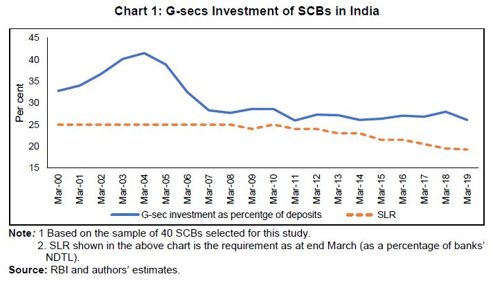 The Indian banking system comprises public sector banks (PSBs), private sector banks (PVBs) and foreign banks. Bank-group wise data indicate that private sector banks had lower NPAs as compared to PSBs while capital adequacy ratio, credit growth, deposit growth, G-secs investment growth, spreads, NIMs, and RoA of private sector banks have exceeded those of the PSBs (Table 2). The faster pace of growth in deposits, credit and G-sec investments of private banks relative to the PSBs reflects the impact of the introduction of new generation private sector banks in the 1990s and their rapid expansion over the next two decades as also the likely impact of the deterioration in asset quality of public sector banks in the recent years on their credit and deposit accretions. As a result, the share of private banks in total credit of all commercial banks nearly trebled from 12.6 per cent in March 2000 to 35.5 per cent in March 2020; their share in total assets of commercial banks also jumped from 12.3 per cent to 32.6 per cent over the same period (Chart 2). Correspondingly, the share of PSBs in the banking system has come down, although they remain predominant. Given the notable differences in the characteristics and growth rates of the two categories of banks over the sample period, we supplement our analysis for all banks with bank-group wise analysis to test the major hypotheses of the paper. 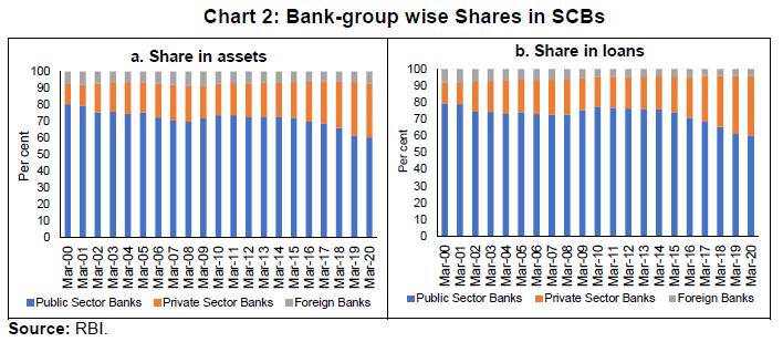 Key variables such as growth in deposits, credit and investments as well as asset quality have exhibited sizeable fluctuations over the sample period. Bank credit growth more than halved between 1999-2011 and 2011-19, along with a sharp moderation in deposit and G-sec investment growth, reflecting inter alia the moderation in nominal GDP growth as well as a drag from the weakening asset quality (Table 3). The slowdown in overall credit growth has also been accompanied with significant compositional shifts, perhaps indicative of asset quality concerns on the one hand and the fast growth of private sector banks on the other hand.5 System-wide NPAs have exhibited a U-shaped pattern over the sample period. Initially, the NPLs declined substantially from over 11 per cent in 2000-01 to a trough of 2.2 per cent in 2007-08 facilitated in part by strong real GDP growth, a jump in the investment activity and high credit growth during this period. The moderation in the pace of economic activity and the asset quality review, however, led to a reversal of this trend in the subsequent years and the NPL ratio increased sharply to around 11 per cent in 2017-18 (back to its 2000-01 level) before some moderation to around 9 per cent in 2018-19 (Chart 3). The deterioration of the asset quality was more pronounced in the case of the PSBs. 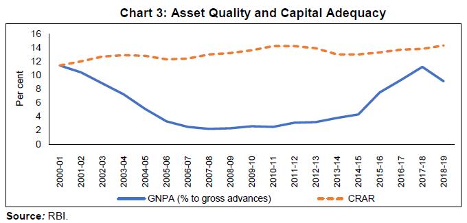 Unlike the significant temporal variation in asset quality, capital adequacy of the overall banking system has seen a modest improvement over the sample period. In India, banks are required to have a minimum CRAR of 9 per cent. Moreover, banks have been required to hold a capital conservation buffer (CCB) since March 2016, which was increased in a phased manner from 0.625 per cent in March 2016 to 1.875 per cent in March 2018.6 In March 2020, the actual CRAR exceeded the then required regulatory minimum (10.875 per cent inclusive of CCB) for all the banks taken together, although a few banks were below the regulatory minimum (RBI, 2020). The size of the banking system increased from 76 per cent to 94 per cent of GDP between the two sub-periods, while the concentration (measured by the share of the top five banks) has remained unchanged. Nominal GDP growth decelerated even as real GDP growth accelerated, indicative of the moderation in inflation. Statutory pre-emptions in the form of CRR and SLR were lower in the second period, while the policy repo rate was higher. Given the notable differences in the banking sector’s performance as well as the underlying macroeconomic performance, we also supplement our baseline analysis with the sample split into two halves (1999-00 to 2010-11 and 2011-12 to 2018-19) to assess the various hypotheses. Scatter plots of bank-wise pooled data suggest a modest negative relationship between government borrowings and banks’ loan growth (Charts 4 and 5). The portfolio of banks exhibits an inclination towards safer assets like G-secs during uncertain times like when economic growth moderates or asset quality of banks deteriorates (Charts 6 and 7). There is a negative correlation between banks’ G-sec investments and RoA, while the correlation between banks’ G-sec investments and NIM is positive (Charts 8 and 9). 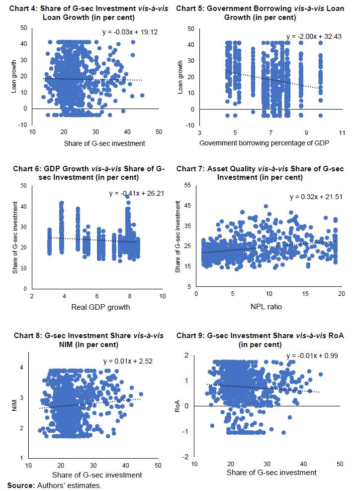 III.2 Methodology A formal analysis of the various hypotheses is undertaken through the econometric specifications set out in equations 1-4 below, with variables selected drawing from the survey presented in Section II: the effect of banks’ investment in government securities and gross market borrowings on loan growth to assess the crowding-out hypothesis (eq. 1); the presence of portfolio rebalancing channel (eq. 2); and the impact of investments in government securities on profitability in terms of NIM (eq. 3) and RoA (eq. 4). In view of the panel nature of the data and the lagged dependent variables, the dynamic panel regressions, following the system generalised method of moments (GMM) approach of Arellano and Bover (1995) and Blundell and Bond (1998), are used to estimate these relationships for the baseline. To correct for downward bias in a finite sample, robust standard errors corrected for small sample bias are used (Windmeijer, 2005).7 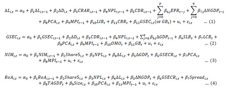 where, ‘i’ refers to the ith bank and ‘t’ refers to the year. For the bank-group wise analysis, the number of panels gets reduced (and equals the number of years), which restricts the use of dynamic panel techniques. Accordingly, the bank-group wise estimation is based on a panel-corrected standard error (PCSE) estimator. For comparability, the sub-period analysis is also based on similar estimation techniques. Variables are defined as follows: ΔL is growth in domestic loans; ΔD is growth in domestic deposits; CRAR is capital to risk weighted assets ratio; NPL is gross non-performing loan ratio (gross non-performing loans to total loans); CDR is credit to deposits ratio (a control for cyclical variation in loans and expected to be negatively related with the loan growth and G-sec investment); EPR is effective policy rate, as a proxy for the cost of loans; ΔGDP/ΔNGDP is growth in real/nominal GDP, as an indicator of the general level of activity in an economy; PCA is a dummy variable which takes value one for a particular bank if the bank has been kept under PCA by the RBI, otherwise zero; MPI is macroprudential indicator, based on a sum of 17 indicators (an increase in MPI indicates a tightening of macroprudential policies, and hence, a rise MPI is expected to moderate loan growth)8; LIB is 3-month US dollar London Inter-Bank Offered Rate (LIBOR), with lower foreign rates making foreign borrowings more attractive and hence lower demand for domestic loans; CRR is cash reserve ratio; SLR is statutory liquidity ratio; LCR is liquidity coverage ratio9; OMO is net open market operations (purchases (+)/sales(-)) conducted by RBI (ratio to GDP); NIM and ROA are bank-wise net interest margin and return on assets, respectively; Share5 is share of top five banks in SCBs’ total assets - a measure of concentration in the banking sector; Size is share of a bank in total assets of all SCBs; TAGDP is total assets of SCBs as a percentage of nominal GDP, as an indicator of the size of the overall banking sector; Spread is bank-wise spread between return on loans and cost of deposits. GSEC, banks’ investments in government securities, is measured by two alternative indicators viz., first, government securities investment of a bank as a percentage of its total assets and second, growth in government securities investment. GSECR is bank-wise ratio of government securities investment in the total assets of the bank. GB is the combined gross market borrowing of the union and state governments as a percentage of nominal GDP. Finally, ui is the bank-specific fixed effect. On the key issue of identification of the crowding-out channel, the existing studies have typically included actual G-sec investments of banks as one of the determinants of loan growth and a negative relationship is seen as supportive of the crowding-out. However, given the balance sheet constraints, if a bank invests more in G-secs, then it has to perforce reduce its lending; this negative relationship may not be a true reflection of the conventional crowding-out channel if banks buy/sell such securities from/to non-banks amidst no fresh borrowings by the government during a given period. As noted earlier, banks’ share in G-sec holdings has declined while that of insurance companies has increased. In view of this, the variable gross government borrowing is better placed to capture the possible crowding-out phenomenon resulting directly from the government absorbing the available pool of financial savings. Gross government borrowings reflect the combined impact of the incremental fiscal deficit during the year plus the rollover of maturing stock of the public debt. While the former is in part endogenous to the business cycle depending upon the cyclicality of the fiscal policy, the maturing part of public debt being rolled over is the outcome of the past debt management policies and, hence, is exogenous to the current business cycle conditions. In this paper, we, therefore, use gross market borrowings to identify the crowding-out to supplement the insights from the existing studies. Based on the studies reviewed in Section II, for equation 1, higher deposit growth, higher CRAR, lower NPAs, higher GDP growth, lower domestic interest rates, higher foreign interest rates, easier macroprudential norms and lower CRR are expected to have a positive impact on loan growth, with higher government borrowings/higher G-sec investments expected to pull down credit growth. For equation (2), higher deposit growth, higher NPAs, weaker growth, higher SLR and LCR, tighter macroprudential norms and higher government borrowings are expected to result in higher G-sec investments by banks while more OMO purchases by the central bank are expected to reduce investments in G-secs by banks. For a bank under PCA, loan growth and G-sec investment growth are expected to be lower and higher, respectively. As regards equations 3 and 4, higher banking system concentration could push up interest margins/profitability and a larger banking system is expected to contain margins/spreads. The impact of asset quality, G-sec holdings, economic activity, loan growth and macroprudential measures is ambiguous and would depend upon the relative importance of the portfolio rebalancing/risk aversion channel. IV.1 Loan Growth and Crowding-out Hypothesis This sub-section explores the determinants of loan growth, with a focus on the impact of banks’ investment in government securities and government market borrowings on loans using equation 1. The regression results are broadly in line with a priori expectations (Table 4, columns 1 to 3). Loan growth is negatively related to the interest rate and the worsening of asset quality, and the impact is statistically significant. Deposit growth, higher capital adequacy and lower CRR have a positive and statistically significant impact on loan growth.10 Higher G-sec investments by banks as well as higher combined gross market borrowings have an adverse impact, statistically significant, on loan growth, in consonance with the crowding-out view.11 Given interest rate, NPAs and GDP growth as controls, the crowding-out due to higher government borrowings would be in addition to that may occur via the interest rate/risk aversion/business cycle channels. Of course, the crowding-out finding could also be in addition to the portfolio rebalancing by banks towards safer assets during economic moderation and rising NPAs – which is examined in the next sub-section. While the results presented in Table 4 suggest the presence of the crowding-out channel, even as we control for risk aversion, capital position and the business cycle, we now evaluate as to whether the size of the crowding-out differs across banks with low/high NPAs/CRAR or across periods of low/high growth. To undertake this analysis, we augment equation 1 with an interaction term of gross market borrowings with a categorical variable for NPAs, or CRAR or GDP growth (equation 5). 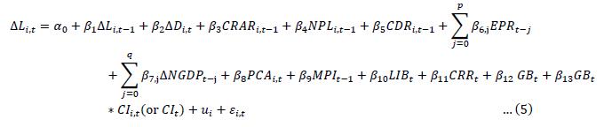 where, CI is a categorical indicator (one variable at a time from the following): Low NPL, High NPL, Low CRAR, High CRAR, Low GDP growth and High GDP growth. These variables are defined as follows: Low NPL and Low CRAR take value 1 when NPL and CRAR are below the respective 25th percentile values (zero otherwise). High NPL and High CRAR take value 1 when NPL and CRAR are above the respective 75th percentile values (zero otherwise). Low GDP growth and High GDP growth take value 1 when nominal GDP growth is below the 25th percentile value and above the 75th percentile value, respectively (zero otherwise). The results presented in Table 5 indicate that the baseline results of Table 4 continue to hold, even when augmented with the interaction terms; for ease of comparison, the baseline results (column 3, Table 4) are reproduced in column 1 in Table 5. The coefficient on gross market borrowings, the key variable, remains negative and statistically significant in all the specifications and supports the continued presence of the crowding-out channel. The coefficient of the interaction term of gross borrowings with high NPA banks is negative and statistically significant while that for low NPA banks is not significant, which suggests that the crowding-out impact is somewhat larger for banks with weaker asset quality. The risk aversion is, thus, more for banks with higher NPLs. As regards capital adequacy, the coefficients of the interaction terms suggest that more capitalised banks resort to less crowding out and are able to undertake more lending to the private sector. Finally, the crowding-out impact moderates during the high growth phase and banks are more willing to support private lending relative to the low growth phase (Table 5).
IV.2 Investments in G-secs and Portfolio Rebalancing by Banks As noted earlier, banks' investments in government securities can increase either due to higher government financing needs (crowding out) or due to the increased risk aversion from uncertain macroeconomic environment and stress in their asset quality (the portfolio rebalancing hypothesis), the latter channel is the focus of this sub-section and the results are presented in Tables 6 and 7 (columns 1 and 2). Weaker economic activity, deterioration in the asset quality and higher SLR increase banks’ investments in government securities investment.12 Gross market borrowings by the government also push up banks’ investment in government securities while OMO purchases by the central bank work in the opposite direction. The negative association of banks’ government securities investment with GDP growth and their asset quality validates the portfolio rebalancing channel. The simultaneous positive and statistically significant association of banks’ investment in government securities with the combined gross market borrowing of governments, despite controls for demand conditions (GDP growth), asset quality (risk aversion) and the mandated SLR/LCR, indicates the presence of crowding-out channel as well (Tables 6 and 7). Higher GDP growth raises loan growth (Tables 5-6) while having a negative impact on G-sec investments (Table 6) suggesting that demand factors play an important role in loan growth. Like bank lending analysis, we now explore as to whether the portfolio rebalancing channel and its quantum differ across banks with low/high NPAs or across periods of low/high growth, by augmenting equation 2 with an interaction term (equation 6 below), with CI being a categorical variable as defined earlier. 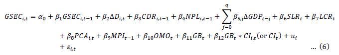 The extended results (Table 8) corroborate the baseline findings of Table 4; for ease of comparison, column 1 in Table 8 repeats the baseline results (column 1, Table 6). The estimates show that banks with weaker asset quality are more risk averse and invest more in G-secs relative to banks with strong asset quality. This is also consistent with the assessment in Table 5 that banks with relatively higher NPLs lend less to the private sector relative to the banks with low NPLs. However, the degree of banks’ support to government borrowings seems to be similar across both high and low growth phases, as the interaction coefficients are statistically insignificant (Table 8).
IV.3 Investment in Government Securities and Margins/Profitability of Banks The impact of investments by banks in government securities on their margins and profitability - net interest margin (NIM) and return on assets (RoA) - is examined in this sub-section using equations 3 and 4 and the empirical results are presented in Tables 9 and 10. Banking concentration, measured by the share of top five banks in SCBs’ total assets, contributes to higher interest margins but not to RoA. A tightening of macroprudential measures lowers banks’ NIMs with a lag. A weakening of the asset quality lowers NIMs and RoA, contrary to John et al. (2016). Better economic growth widens NIM but does not seem to have any significant impact on RoA. Finally, the share of government securities investment in banks’ total assets has a significant positive impact on both NIM and RoA, suggesting better risk-adjusted return on investments in view of lower risk provisions for government securities, although the subsequent analysis suggests that these findings are primarily driven by public sector banks. IV.4 Robustness Analysis This section undertakes robustness checks in a number of ways. First, to deal with the outliers, the data has been winsorised 10 per cent from each side relative to 5 per cent winsorisation in the baseline results. Overall, the results are broadly similar to the baseline results, albeit with some differences (Table 4, columns (4)-(6); and Tables 6-7 and 9-10, columns (3)-(4)). The impact of growth in banks’ G-secs investment and gross market borrowings of government on loan growth becomes higher and more statistically significant (Table 4, columns (4)-(6)). The impact of the deterioration in asset quality on banks’ decision to increase G-secs investment becomes statistically significant (Table 6, columns (3)-(4)).
Second, as an alternative to the winsorisation technique, the data were trimmed by dropping outliers (5 per cent from each side). The broad inferences are similar to the baseline results (Table 4, columns (7)-(9); and Tables 6-7 and 9-10, columns (5)-(6)). Amongst the variables of interest, the impact of the share of banks’ G-secs investment in the total assets on loan growth turns statistically significant. Furthermore, the results related to the improved RoA of banks on account of an increased share of G-secs in their assets portfolio remained similar to that of the baseline result. Third, in view of the earlier noted differences in the governance structure, the pace of expansion, asset quality, and the profitability metrics, the empirical analysis is attempted separately for the PSBs and private sector banks groups. While the results for the two bank groups are broadly in conformity with the baseline, there are a few notable differences.13 The adverse impact of growth in G-secs investment on bank credit is somewhat higher in the case of PSBs. Higher government borrowings have a negative statistically significant impact on bank credit only in the case of private sector banks, perhaps reflecting the faster growth in the balance sheet size of these banks and the initial overhang of excess SLR securities with PSBs. Private banks’ lending is more sensitive to the movements in the policy interest rate relative to PSBs while that of PSBs is somewhat more influenced by the state of the economy as captured by nominal GDP growth (Annex, Table A2). A worsening of the asset quality drives PSBs to increase their holdings of G-secs while this channel is absent for private banks – thus, the risk aversion channel is driven by PSBs. Tighter macroprudential measures lead private banks to increase their G-sec holdings (Annex, Table A3). Higher G-sec investments increase the NIMs of PSBs but depress the NIMs of private banks, perhaps indicative of the overhang of NPAs in the PSBs while private banks seem to generate more returns from their lending operations relative to G-sec investments in consonance with the conventional wisdom (Annex, Table A4). Similarly, the significant positive impact of G-secs investment on profitability (RoA) of banks on account of better risk adjusted return on G-secs investment is confined to the public sector banks (Annex, Table A5). Fourth, to assess the possible impact of ongoing structural changes in the banking system and the Indian economy on the credit, investment, margins, and profitability dynamics, we split our sample into two halves (1999-00 to 2010-11 and 2011-12 to 2018-19). The results indicate that bank credit has turned somewhat more sensitive to capital adequacy, deposit growth and demand conditions (the pace of economic activity) and less sensitive to asset quality and interest rates in the latter period (Annex, Table A6). Higher government borrowings lead to relatively higher investments by banks in G-secs in the latter period (Annex, Table A7). NPLs depress NIMs and RoA relatively more in the latter period. Higher G-sec investments have had a more negative impact on NIMs and RoA in the recent period, perhaps reflective of the growing role of private sector banks discussed earlier for whom NIMs/RoA are negatively related or not sensitive to G-sec investments (Annex, Table A8 and A9). The Indian financial system is bank dominated and banks play a critical role in the intermediation of financial savings towards productive investment. At the same time, given the fiscal deficits, the governments (both centre and states) depend critically upon banks to finance their deficits through market borrowings. Thus, banks need to allocate their deposits between financing the government needs as well as that of the private sector. While the regulatory SLR requirement mandates banks to hold a specified fraction of their deposits and liabilities in government securities, banks in India often hold government securities over and above the required SLR and this excess varies significantly across banks as well as over time. Banks could be holding these excess securities for a variety of reasons like liquidity management (given these securities are highly liquid and the excess SLR securities allow banks to borrow from RBI under the liquidity adjustment facility) and their risk appetite (domestic government securities are risk-free and could be particularly attractive to banks in economic downturns or to banks with high non-performing loans). Higher investment by banks in government securities implies a reduction in funds available for lending to the private sector. Against this backdrop, this paper analysed the determinants of loan growth and investment in government securities and the impact of banks' investment in government securities on their profitability. The empirical analysis indicates that weak economic conditions and stressed asset quality encourage banks to increase their investments in government securities suggesting the presence of a portfolio rebalancing channel and the impact is somewhat higher for banks with more stressed asset quality. At the same time, increased investment by banks in government securities in the face of higher government borrowings crowds-out private credit and the effect is stronger for banks with higher non-performing loans while it gets ameliorated for more capitalised banks and during periods of stronger economic growth. The empirical analysis, thus, suggests the presence of both portfolio rebalancing and crowding-out channels at play and policies aimed at strengthening the asset quality and capital position of the banks can lead to an enhanced flow of bank credit to the productive sectors. An increase in the share of government securities in banks’ asset portfolio is found to have a favourable impact on their banks’ profitability, indicating a better risk-adjusted return on investment, although this result seems to be driven by public sector banks. The COVID-19 pandemic led to a sharp loss of output in 2020-21. The adverse impact on the overall economic activity was somewhat offset by a countercyclical fiscal policy which in turn was mirrored in higher government borrowings on the back of the fall in revenues and higher expenditures. Reflecting these developments, banks’ investment in government securities increased while credit growth was subdued consistent with the paper’s evidence of portfolio rebalancing; the crowding-out channel was somewhat less important since the countercyclical fiscal policy was necessitated by weak domestic demand in the aftermath of the pandemic. Proactive monetary, liquidity and regulatory measures by the Reserve Bank ensured continued credit flows not only through banks but also through market instruments like corporate bonds and commercial paper, facilitating a revival of economic activity (Das, 2021; RBI, 2021). Thus, the central bank’s regular market operations in sync with the monetary policy stance helped the banking system to balance the financing needs of the various sectors of the economy. This study has focused on credit and investment dynamics of commercial banks. With the increasing role of non-bank players in financing economic activities in India, the paper’s work can be further extended by covering other financial sector players, such as, non-bank financial institutions. @ Sanjay Singh is Director in Department of Statistics and Information Management while Garima Wahi and Muneesh Kapur are Assistant Adviser and Adviser, respectively, in Monetary Policy Department, Reserve Bank of India. 1 The views expressed in the paper are those of the authors and not necessarily those of the institution to which they belong. Comments from D.P. Rath, Sitikantha Pattanaik, Snehal Herwadkar, Jai Chander, Pankaj Kumar and Sadhan Kumar Chattopadhyay and an anonymous reviewer and assistance with data processing from Nilesh Deshmukh are gratefully acknowledged. The usual disclaimer applies. * Corresponding author (sanjays@rbi.org.in). 2 All public and private sector banks (except two newly created private banks) were included in the sample. These banks had a share of 94 per cent in assets of all the SCBs in India in 2018-19. 3 https://dbie.rbi.org.in/DBIE/dbie.rbi?site=home 4 Winsorisation replaces the extreme values in the data by the specified percentiles; in our case, the bottom 5 per cent and the top 5 per cent data values for each variable are replaced by the 5th and the 95th percentile values of that data series. 5 Banks’ credit to industry (per cent to overall non-food credit) initially rose from 38.9 per cent in March 2008 to 45.8 per cent in March 2013 but then declined sharply in the subsequent years to 31.5 per cent in March 2020. On the other hand, the share of personal loans exhibited an opposing trend: it initially fell from 23.7 per cent in March 2008 to 18.2 per cent in March 2012 but then recovered to 27.7 per cent in March 2020. The share of services has remained relatively stable and increased from 24.9 per cent in March 2008 to 28.2 per cent in March 2020. 6 The implementation of the last tranche of 0.625 per cent of CCB which was due from March 31, 2019 was deferred to October 2021. 7 All estimations are done using the software Stata (version 16.0). 8 Out of the 17 indicators in the MPI, as many as 16 pertain to banks (except ‘tax measures’ which is anyways 0 for India). So, the MPI is effectively focussed on banks. 9 LCR used in the paper is the proportion required by commercial banks to be held in the respective years – 60, 70, 80, 90 and 100 per cent in 2015, 2016, 2017, 2018 and 2019, respectively. 10 Apart from making loans to the private sector, banks have the option of investing in ‘bonds and debentures’ of firms/corporates. However, this variable did not turn out to be statistically significant in our regressions. Perhaps, this reflects that ‘bonds and debentures’ have a very low share in banks’ assets (less than 3 per cent on average during the sample period of the study). 11 The share of G-sec investments in bank’s total assets, however, did not have any statistically significant impact on loan growth. 12 Apart from required SLR, bank’s investments in G-secs can also be motivated by their investment preferences like holding them to maturity or mainly for sale. For the former group, RBI’s regulatory stipulations/dispensations with regard to “held to maturity” (HTM) portfolio can thus be an important determining variable in the regression. To examine this channel, we tried regressions with HTM in lieu of SLR as an explanatory variable; however, it did not turn out to be statistically significant. This perhaps reflects that HTM, although it exhibits high co-movement with SLR, was unchanged for a large part (the first 13-14 years) of the sample period. 13 As noted earlier, bank-group wise analysis leads to a reduction in the number of panels and hence these estimates are based on static panel techniques, with standard errors corrected for heteroscedasticity and autocorrelation within panels. For comparability, we also report estimates for the full sample and these are broadly similar to the dynamic panel estimates reported earlier. References Acharya, V. V. (2018). Why less can be more: On the crowding-out effects of government financing. Speech at 16th K P Hormis Commemorative Lecture organised by the Federal Bank, November 17th. Al-Homaidi, E. A., Tabash, M. I., Farhan N. H. S., & Almaqtari F. A. (2018). Bank-specific and macro-economic determinants of profitability of Indian commercial banks: A panel data approach. Cogent Economics & Finance, 6:1, 1548072, DOI: 10.1080/23322039.2018.1548072. Alam, Z., Alter, A., Eiseman, J., Gelos, G., Kang, H., Narita, M., Nier, E., & Wang, N. (2019). Digging deeper – Evidence on the effects of macroprudential policies from a new database. Working Paper 66, International Monetary Fund. Alani, E. M. A. A. (2006). Crowding-out and crowding-in effects of government bonds market on private sector investment (Japanese case study). Discussion Paper 74, Institute of Developing Economies. Alihodžić, A., & Ekşi İ. H. (2018). Credit growth and non-performing loans: Evidence from Turkey and some Balkan countries. Eastern Journal of European Studies, Vol. 9, Issue 2, pp. 229-249. Araujo, J., Patnam, M., Popescu, A., Valencia, F., & Yao, W. (2020). Effects of macroprudential policy: Evidence from over 6,000 estimates. Working Paper 67, International Monetary Fund. Arellano, M., & Bover, O. (1995). Another look at the instrumental variable estimation of error-components models. Journal of Econometrics, Vol. 68, Issue 1, pp. 29–51. Ariccia, G. D., Rabanal, P., & Sandri, D. (2018). Unconventional monetary policies in the Euro area, Japan, and the United Kingdom. Journal of Economic Perspectives, Vol. 32, No. 4, pp. 147-172. Becker, B., & Ivashina, V. (2018). Financial repression in the European sovereign debt crisis. Review of Finance, Vol. 22, Issue 1, pp. 83–115. Berger, A. N., & Udell, G. F. (2003). The institutional memory hypothesis and the procyclicality of bank lending behaviour. Working Paper 125, Bank for International Settlements. Bernanke, B. S., & Blinder, A. S. (1992). The federal funds rate and the channels of monetary transmission. The American Economic Review, Vol. 82, No. 4, pp. 901-921. Berrospide, J. M., & Edge, R. M. (2010). The effects of bank capital on lending: What do we know, and what does it mean?. International Journal of Central Banking, Vol. 6, No. 4, pp. 5-54. Blundell, R., & Bond, S. (1998). Initial conditions and moment restrictions in dynamic panel data models. Journal of Econometrics, Vol. 87, Issue 1, pp. 115–143. Bouis, R. (2019). Banks’ holdings of government securities and credit to the private sector in emerging market and developing economies. Working Paper 224, International Monetary Fund. Borio, C., & Gambacorta, L. (2017). Monetary policy and bank lending in a low interest rate environment: Diminishing effectiveness?. Journal of Macroeconomics, Vol. 54, Part B, pp. 217–231. Brahmaiah, B., & Ranajee (2018). Factors influencing profitability of banks in India. Theoretical Economics Letters, 8, pp. 3046-3061. Budnik, K. (2020). The effect of macroprudential policies on credit developments in Europe 1995-2017. Working Paper Series 2462, European Central Bank. Caruana, J. (2002). Asset price bubbles: Implications for monetary, regulatory and international policies. Speech at Federal Reserve Bank of Chicago, April 24th. Cucinelli, D. (2015). The impact of non-performing loans on bank lending behaviour: Evidence from the Italian banking sector. Eurasian Journal of Business and Economics, Vol. 8, No. 16, pp. 59-71. Dahir, A. M., Mahat, F., Razak, N. H. A., & Bany-Ariffin, A. N. (2019). Capital, funding liquidity, and bank lending in emerging economies: An application of the LSDVC approach. Borsa Istanbul Review, Vol. 19, Issue 2, pp.139-148. Das, S. (2021). Towards a stable financial system. Nani Palkhivala Memorial Lecture, Reserve Bank of India Bulletin, February, pp.17-22. Egesa, K. A., Ocaya, B. M., Atuhaire, L. K., Mwanga, Y., Makumbi, T. N., & Mugisha, X. (2015). Determinants of investment in government securities by banks in Uganda. International Journal of Economics, Finance and Management Sciences, Vol. 3, No. 3, pp. 294-302. Gambacorta, L., & Murcia, A. (2019). The impact of macroprudential policies and their interaction with monetary policy: An empirical analysis using credit registry data. IFC Bulletins, Are Post-crisis Statistical Initiatives Completed?, Vol No. 49, Bank for International Settlements. Gómez, E., Murcia, A., Lizarazo, A., & Mendoza, J. C. (2020). Evaluating the impact of macroprudential policies on credit growth in Colombia. Journal of Financial Intermediation, Vol. 42, Article 100843. Goyal, A., & Verma, A. (2018). Slowdown in bank credit growth: Aggregate demand or bank non-performing assets?. Margin: The Journal of Applied Economic Research, Vol. 12, Issue 3, pp. 257-275. Hauner, D. (2009). Public debt and financial development. Journal of Development Economics, Vol. 88(1), pp. 171–183. John, J., Mitra, A. K., Raj, J., & Rath, D. P. (2016). Asset quality and monetary transmission in India. Reserve Bank of India Occasional Papers, Vol. 37, No.1&2, pp. 35-62. Kashyap, A. K., & Stein, J. C. (2000). What do a million observations on banks say about the transmission of monetary policy?. The American Economic Review, Vol. 90, No. 3, pp. 407-428. Keeton, W. R. (1994). Causes of the recent increase in bank security holdings. Economic Review, Federal Reserve Bank of Kansas City, Vol. 79 (QII), pp. 45-57. --- (1999). Does faster loan growth lead to higher loan losses?. Economic Review, Federal Reserve Bank of Kansas City, Vol. 84 (QII), pp. 57-75. Kohlscheen, E., Murcia, A., & Contreras, J. (2018). Determinants of bank profitability in emerging markets. Working Paper 686, Bank for International Settlements. Mohan, R. (2009). Monetary policy in a globalized economy: A practitioner’s view. Oxford University Press, New Delhi. Mohanty, B. K., & Krishnankutty, R. (2018). Determinants of profitability in Indian banks in the changing scenario. International Journal of Economics and Financial Issues, Vol. 8, Issue 3, pp. 235-240. Muduli, S., & Behera, H. (2020). Bank capital and monetary policy transmission in India. Working Paper 12, Reserve Bank of India. Olszak, M., Pipień, M., Roszkowska, S., & Kowalska, I. (2014). The effects of capital on bank lending in large EU banks – The role of procyclicality, income smoothing, regulations and supervision. Working Paper Series 5, University of Warsaw, Faculty of Management. Ongena, S., Popov, A., & Horen, N. V. (2019). The invisible hand of the government: Moral suasion during the European sovereign debt crisis. American Economic Journal: Macroeconomics, Vol. 11, No. 4, pp. 346–379. Petria, N., Capraru, B., & Ihnatov, I. (2015). Determinants of banks’ profitability: Evidence from EU 27 banking systems. Procedia Economics and Finance, Vol. 20, pp. 518-524. Raj, J., Rath, D.P., Mitra, P., & John, J. (2020). Asset quality and credit channel of monetary policy transmission in India: Some evidence from bank-level data. Working Paper 14, Reserve Bank of India. Rajan, R. G. (1994). Why bank credit policies fluctuate: A theory and some evidence. The Quarterly Journal of Economics, Oxford University Press, Vol. 109, Issue 2, pp. 399-441. Reserve Bank of India (2020). Report on Trend and Progress of Banking in India 2019-20, December. --- (2021). “Governor’s Statement, April 7, 2021”. Rodrigues, A. P. (1993). Government securities investments of commercial banks. Quarterly Review, Federal Reserve Bank New York, Vol. 18, pp. 39-53. Saif, A. Y. H. (2014). Financial performance of the commercial banks in the Kingdom of Saudi Arabia: An empirical insight. Thesis for Master of Finance, Universiti Utara Malaysia, Available at http://etd.uum.edu.my/4587/. Serven, L. (1996). Does public capital crowd out private capital?: Evidence from India. Policy Research Working Paper 1613, The World Bank. Tan, T. B. P. (2012). Determinants of credit growth and interest margins in the Philippines and Asia. Working Paper 123, International Monetary Fund. Tovar, C. E., Garcia-Escribano, M., & Martin, M. V. (2012). Credit growth and the effectiveness of reserve requirements and other macroprudential instruments in Latin America. Working Paper 142, International Monetary Fund. Windmeijer, F. (2005). A finite sample correction for the variance of linear efficient two-step GMM estimators. Journal of Econometrics, Vol. 126, Issue 1, pp. 25-51. Zampara, K., Giannopoulos, M., & Koufopoulos, D. N. (2017). Macroeconomic and industry-specific determinants of Greek bank profitability. International Journal of Business and Economic Sciences Applied Research, Vol. 10, Issue.1, pp. 13-22. Zhu, F. (2011). Credit and business cycles: some stylised facts. Bank for International Settlements (available at https://www.suomenpankki.fi/globalassets/en/research/seminars-and-conferences/conferences-and-workshops/documents/fdr2011/fdr2011_zhu_paper.pdf).
| |||||||||||||||||||||||||||||||||||||||||||||||||||||||||||||||||||||||||||||||||||||||||||||||||||||||||||||||||||||||||||||||||||||||||||||||||||||||||||||||||||||||||||||||||||||||||||||||||||||||||||||||||||||||||||||||||||||||||||||||||||||||||||||||||||||||||||||||||||||||||||||||||||||||||||||||||||||||||||||||||||||||||||||||||||||||||||||||||||||||||||||||||||||||||||||||||||||||||||||||||||||||||||||||||||||||||||||||||||||||||||||||||||||||||||||||||||||||||||||||||||||||||||||||||||||||||||||||||||||||||||||||||||||||||||||||||||||||||||||||||||||||||||||||||||||||||||||||||||||||||||||||||||||||||||||||||||||||||||||||||||||||||||||||||||||||||||||||||||||||||||||||||||||||||||||||||||||||||||||||||||||||||||||||||||||||||||||||||||||||||||||||||||||||||||||||||||||||||||||||||||||||||||||||||||||||||||||||||||||||||||||||||||||||||||||||||||||||||||||||||||||||||||||||||||||||||||||||||||||||||||||||||||||||||||||||||||||||||||||||||||||||||||||||||||||||||||||||||||||||

ఈ పేజీని షేర్ చేయండి:


భారతీయ రిజర్వ్ బ్యాంక్ మొబైల్ అప్లికేషన్ను ఇన్స్టాల్ చేయండి మరియు తాజా వార్తలకు త్వరిత యాక్సెస్ పొందండి!
మా యాప్ను ఇన్స్టాల్ చేయడానికి QR కోడ్ను స్కాన్ చేయండి


పేజీ చివరిగా అప్డేట్ చేయబడిన తేదీ:


