 IST,
IST,


Financial Conditions Index for India: A High-Frequency Approach
|
by Pulastya Bandyopadhyay, Avnish Kumar, Pankaj Kumar and Indranil Bhattacharyya^ This article attempts to construct a financial conditions index (FCI) for India at daily frequency, using select indicators from the money, G-sec, corporate bond, equity, and forex markets. The primary objective is to construct a composite indicator that tracks overall conditions in financial markets at a high frequency. The FCI assesses the degree of relatively tight or easy financial market conditions with reference to its historical average since 2012. The estimated FCI traces movements in financial conditions in India across both periods of relative calm as well as crisis episodes. The index suggests that in the aftermath of the pandemic, exceptionally easy financial condition was driven by the combined impact of amiable conditions across all market segments. Financial conditions continued to remain relatively easy since mid-2023 before firming up from November 2024. In the current financial year, however, it has remained congenial riding on a buoyant equity market and a money market suffused with liquidity. Introduction A financial conditions index (FCI) is a summary measure that encapsulates the information contained in a broad array of financial variables and helps to gauge the relative tightness or ease in overall financial conditions. Monetary policy actions impact financial conditions through the usual channels of monetary transmission although financial conditions, independent of policy decisions, often change because of news events, macroeconomic data releases and market microstructure issues. Thus, the FCI is a valuable input for monetary policy as it provides lead information on real economic activity, over and above the direct effects of monetary policy (Hatzius et al., 2010). It can, therefore, serve as a guide on the effective stance of policy (Bowe et al., 2023). One of the key takeaways of the Global Financial Crisis (GFC) was that financial innovation had made it difficult to capture broad financial conditions in a small number of variables covering traditional financial markets. Thus, FCI emerged as a key tool in assessing macro-financial conditions in the post-GFC era. Apart from gauging the state of financial markets, FCI has been used by policymakers and practitioners to predict the future state of the economy as well as the risks associated with economic forecasts. The use of FCI in the conduct of monetary policy, forecasting models and stress testing is still limited among emerging market economy (EME) central banks compared to their advanced economy (AE) counterparts. Most studies in the Indian context relied on monthly or quarterly data to construct FCI, thus constraining their use in reacting to sudden market developments, real time policy making and forecasting. In view of the above, this article attempts to construct a new FCI for India at daily frequency using select indicators from various market segments. The primary objective is to construct a summative measure that is able to track overall conditions in financial markets. The paper is structured in the following manner: Section II presents an overview of the existing literature on construction of FCIs in the global as well as the Indian context. The choice of variables and the empirical methodology are discussed in Section III. Section IV evaluates the robustness of the derived measure and discusses its features and drivers while Section V presents some concluding observations. The following discussion provides an overview of the existing literature on financial condition indices, with a focus on the methodological approaches followed by global as well as Indian studies in this area. A vast literature has proliferated exploring the construction of FCIs across AEs; however, EMEs in general and India in particular have relatively drawn limited attention. As mentioned before, the concept of FCI gained prominence in the aftermath of the GFC. International institutions and multilateral bodies like the International Monetary Fund (IMF), Organization for Economic Co-operation and Development (OECD), Bank for International Settlements (BIS) and several AE central banks have since refined and institutionalised FCIs as part of their macro-financial surveillance toolkit. Early work derived FCIs for the G7 countries as a weighted average of the short-term real interest rate, the effective real exchange rate, and real property and share prices by looking at reduced form coefficient estimates and vector autoregression (VAR) impulse responses (Goodhart and Hofmann, 2001). A Goldman Sachs FCI was constructed as a weighted sum of a short-term bond yield, a long-term corporate yield, exchange rate, and a stock market variable (Dudley and Hatzius, 2000; Dudley et al., 2005). Deutsche Bank uses principal component analysis (PCA) for constructing the index from a set of seven financial variables that included the exchange rate, bond, stock, and housing market indicators (Hooper et al., 2007). Developed in 2008, the OECD FCI is a weighted sum of six financial variables with their weights being in proportion to their impact on GDP (Guichard and Turner, 2008; Guichard et al., 2009). Similarly, Citi Financial Conditions Index is a weighted sum of six financial variables, viz., corporate spreads, money supply, equity values, mortgage rates, the trade-weighted dollar, and energy prices. The weights were determined according to reduced form forecasting equations of the Conference Board’s index of coincident indicators (D’Antonio, 2008). The Bloomberg FCI index, on the other hand, is an equally weighted sum of three major sub-indices including indicators from money, bond, and equity markets (Rosenberg, 2009). Vector autoregressions and impulse-response functions were used to construct an FCI for the US; in addition to the usual indicators, credit availability from bank lending survey was also used to construct the FCI (Swiston, 2008). An FCI for the Asian economies was constructed based on an unrestricted VAR using financial variables viz., private sector credit growth, real lending rates, interest rate spreads, lending standards, equity price movements and real effective exchange rate changes (IMF, 2010). Subsequently, IMF staff economists have combined this method with a dynamic factor model (DFM) to further develop an index for the Asian economies (Osorio et al., 2011). These institutions have periodically improved the methodology to construct their individual FCIs. Several studies on the US, the Euro Area, Sweden, Germany and Norway further refined the methodology and updated their indices (Hatzius et al., 2010; Brave and Butters, 2011; Alsterlind et al., 2020; Metiu, 2022; Bowe et al., 2023). In the Indian context, the work on FCI gained traction over the past decade. A financial conditions index was first developed for India using monthly data on money, bond, foreign exchange and stock markets, using a PCA approach (Shankar, 2014). Subsequently, a monthly financial conditions composite indicator was constructed based on ten indicators by using PCA to extract the top factors containing maximum information (Roy et al., 2015). VAR-based weighted sum approach for five indicators as well as PCA using a larger set of ten indicators was used to estimate FCI at a monthly frequency (Khundrakpam et al., 2017). Similarly, a VAR-based weighted sum approach and a DFM of five indicators were employed to compute FCI at a quarterly frequency (Kumar et al., 2022). In contrast, the CII-IBA Financial Conditions Index (FCI) is based on a quarterly Financial Conditions Expectation Survey of major banks and financial institutions on their expectations of key financial and economic variables that determine financial conditions in the Indian economy. The construction of FCIs differ across studies in terms of the aim of the measure, indicators selected, data frequency and econometric methodologies. The range of indicators included in the construction of various FCIs differ across studies, although there are some commonalities. Most FCIs include some measures of interest rates, risk premia, equity market performance, exchange rates and volatility measures. In terms of methodology, while early studies mostly used the weighted-sum approach and PCA, recent literature has relied mostly on DFM or time-varying parameter models to construct FCIs. In the weighted-sum approach, the weight of the chosen indicator is generally assigned based on the impact it has on the target variable such as the real GDP. These estimates or weights have been generated in a variety of ways, including simulations using large-scale macroeconomic models, VAR models, or reduced-form demand equations. On the other hand, the PCA extracts a common factor from a group of several financial variables. PCA is purely a static estimation tool and does not incorporate information along the time dimension for constructing the index. In contrast, DFM allows for the incorporation of time-series dynamics of some finite order to extract the latent factors (Brave and Butters, 2011). III. Constructing a Financial Conditions Index III.1 Selection of Variables The existing literature provides valuable insights for selecting appropriate variables in the construction of FCI. An FCI for India is constructed using twenty financial market indicators at daily frequency. The chosen indicators represent five market segments, viz., (i) the money market; (ii) the Government securities (G-sec) market; (iii) the corporate bond market; (iv) the forex market; and (v) the equity market (Chart 1). To some extent, the selection of variables is also influenced by the primary objective of this study, i.e., to construct a high frequency FCI, thus necessitating the use of financial indicators that are readily available at a daily frequency.  a. Money Market The money market assumes special significance in gauging financial market conditions as it is the fulcrum of monetary policy operations – most central banks operationalise monetary policy via the overnight money market. Monetary policy actions and stance get seamlessly conveyed to the overnight market, which then propagates through the money market spectrum. Hence, the operating target of monetary policy in India, i.e., the weighted average call rate (WACR) becomes an important indicator of the money market. The rates in the collateralised segment of the overnight market track the movements in WACR. Also, the volume in collateralised money market – triparty repo and market repo – are significantly higher, which necessitates their inclusion; hence, the weighted average money market rate1 (WAMMR) is considered for our analysis. The WAMMR captures the cost of overnight funds for banks and non-banks; however, it is not the level of WAMMR but its deviation from the policy repo rate which is reflective of financial conditions in the overnight money market. Hence, we include WAMMR spread over the policy repo rate as one of the indicators. Volatility in WAMMR and liquidity conditions [net balances under the liquidity adjustment facility (LAF) adjusted for net demand and time liabilities (NDTL)] are also considered. In order to capture the credit risk at the short end of the interest rate spectrum, the spread of 3-month CP rate over 3-month T-bill rate is also included. b. G-sec Market The importance of the G-sec market lies in providing the risk-free term structure for pricing of financial instruments issued by other sectors of the economy. It also provides an avenue for raising the financing requirements of the government in meeting the budgetary gap. Any change in G-sec yields would alter the borrowing cost for the government as well as other market players. Hence, indicators which capture the dynamics of G-sec market are included in the FCI. G-sec market is represented by the latent factors of the sovereign yield curve i.e., level, slope, and curvature. The level2 of the yield curve has a positive association with financial conditions as an increase in interest rate increases financing costs, thus tightening financial conditions. The slope3 of the yield curve is the term spread that captures the difference between long term and short-term yields. Theoretically, if long-term rates are notably higher than short-term rates, it indicates that market expects short-term rates to increase in the near future, leading to tighter financial conditions. Similarly, higher curvature4 implying greater concavity of the yield curve and higher interest rates in the middle of the term structure suggests tighter financial conditions, besides reflecting market segmentation and preferred habitat of investors. Contrary to theoretical prediction, however, higher slope and curvature contribute to easier financial conditions in our empirical exercise, as they mostly reflect very low short-term rates. c. Corporate Bond Market The corporate bond market provides an alternative avenue to raise medium and long-term funds for private sector participants. Hence, bond yields serve as a barometer for the health of the credit market. The credit spreads – difference between corporate bond yields and G-sec yields of corresponding maturity – offer insights into financial conditions. The change in credit spreads often signal change in credit risk perceptions and investor sentiments about economic conditions. This segment is represented by credit risk indicators across various ratings and tenors. Increase in credit risk premia reflects higher risk associated with the private sector vis-à-vis the government. A higher credit risk premium is indicative of tighter financial conditions making borrowing more expensive for corporates. d. Forex Market Forex market indicators include India-US yield differential, INR return5, 1-month forward premia and 1-month at-the-money (ATM) implied volatility to capture financial conditions in the foreign exchange market. Higher India-US yield differential and rupee depreciation are assumed to be associated with tighter financial conditions in our analysis. This is because an increase in yield differential reflects relatively higher domestic interest rate, which compensates for the expected rupee depreciation and country risk premium under the interest rate parity condition. The impact of rupee depreciation works through trade and finance channels. Since, the trade channel works with a lag and is found to be weaker, we have considered the finance channel to be predominant in the short run. Rupee depreciation leads to an increase in debt servicing cost, thus leading to tighter financial conditions. Further, 1-month ATM implied volatility is a measure of market expectations of future volatility of the currency exchange rate. Higher values depict more volatility and hence more uncertainty. Increase in 1-month ATM volatility and forward premia is associated with tighter financial conditions. e. Equity Market The equity market is represented mostly by price indicators capturing returns and volatility. The equity market indicators are return [Sensex, midcap and small cap return, price to earnings (PE) ratio] and volatility (India VIX). Conditions in the stock market affect the ability of corporates to raise fresh capital. Higher returns attract greater FII and FPI inflows, which affect valuations and have a positive impact on the overall market sentiment. Higher stock prices enhance wealth, which may boost consumer spending and business investment. Therefore, higher return in the equity market is associated with easier financial conditions. The PE ratio is indicative of how much investors are willing to pay per rupee of earnings. Higher values are realised when market sentiments are buoyant. Decline in the PE ratio and increase in volatility are associated with tighter financial conditions. Hence, the confluence of widening spreads in money and bond market, elevated market volatility, diminishing asset returns and shrinking volumes is reflective of a tightening in overall financial conditions. III.2 Empirical Methodology This study uses daily data of twenty financial market indicators for the period January 1, 2012 to May 30, 2025 to construct FCI for India. All indicators are factored into the index in such a manner so that an increase in these indicate a tightening of financial conditions. Accordingly, the transformations are carried out for select indicators so that a higher value of the transformed variable indicates tighter financial conditions (Appendix Table 1). We employ both PCA and DFM approach to estimate the FCI. (i) PCA Approach We use PCA to extract the common factor from the selected twenty indicators. PCA is a statistical technique used to reduce the dimensionality of a dataset by transforming a large set of correlated variables into a smaller set of uncorrelated components. These PCs are linear combinations of the original variables that capture the maximum variance in the data, thereby retaining most of the information embedded in the data while reducing its dimensionality. The loadings associated with each principal component – derived from the eigenvectors of the data’s covariance or correlation matrix – are used to construct indices or scores that summarize the information contained in the original variables.
In our analysis, the first principal component explains about 40 per cent of the total variation in the chosen indicators. The variable loadings (Appendix Table 2) are observed to be on expected lines for most indicators, except for those of the slope and curvature of the yield curve. Contrary to theoretical prediction, higher slope and curvature contribute to easier financial conditions in our empirical exercise, as they mostly reflect lower rates at the short end of the yield curve. The contributions of the various market segments in the FCI are found to be well distributed (Table 1). Since PCA is purely a static estimation tool and does not incorporate information along the time dimension, we also use DFM to estimate the FCI. (ii) DFM Approach DFM is widely used to extract a common set of underlying trends which captures the bulk of covariation among a large set of time series indicators. DFM lends itself naturally to the problem of index construction, as in a DFM with a single underlying unobserved factor, the estimate of the latent factor stands for an index of the co-movement in the indicators (Stock and Watson, 2016). We use a DFM framework for the construction of the FCI: 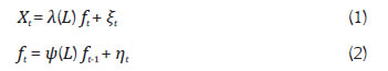 where, Xt is a N × 1 vector of observed time series variables, variations in which are explained by a reduced number of unobserved (latent) factors and mean-zero idiosyncratic components ξt. The lag polynomials λ(L) and ψ(L) are N × q and q × q matrices, respectively, and ηt is a q × 1 vector of serially uncorrelated mean zero innovations to the factors. The idiosyncratic disturbances are assumed to be uncorrelated with factor innovations at all leads and lags, that is E(ξt η’t–k) = 0 for all k. The ith row of λ(L) is the dynamic factor loading for the ith series Xit. The q unobserved (latent) factors ft are the source of co-movement across observed indicators, which is the identification strategy to estimate this state-space model. We estimate the DFM for a single common factor, which is the FCI, and allow for two lags in Equation (2).6 Following the literature, we employ a two-step estimator in which the first step involves estimating the parameters of the model using an ordinary least square (OLS) on principal components and, in the next step, the factors are estimated using the Kalman filter and smoother (Doz et al., 2011). The factor loadings for the chosen indicators are presented in Appendix Table 3. In our empirical exercise, the FCI estimated using PCA broadly tracks the FCI estimated using the DFM approach. We present our results for the FCI obtained from the DFM. FCI is a broader metric of the state of financial markets as it captures the interaction of financial conditions and economic activity. The index gives a sense of how tight or loose financial markets are relative to their historical average. The FCI provides a metric based on its historical average; in this context, a zero value of FCI corresponds to a financial system operating at the historical average level of all the financial indicators included in the FCI, i.e., essentially, a “neutral” financial condition. A higher positive value of the FCI is indicative of tighter financial conditions. To present our results, we use the standardised FCI. Standardisation helps in interpreting the changes in financial condition in terms of standard deviation units. For example, within our sample period, financial condition was at its tightest at end-July 2013 during the taper tantrum episode, with the estimated standardised FCI at 2.826 – almost a 3-standard deviation tightening relative to the historical average. On the other hand, the FCI stood at -2.197 at mid-June 2021 – indicating the exceptionally easy financial conditions post-Covid. Chart 2 plots the estimated FCI and the drivers7 of the financial conditions. To assess the reliability of the newly constructed index, the following analysis examines the performance of the index through a narrative approach.  The Index through History One way to evaluate the newly constructed index as a measure of financial conditions is to follow a narrative approach and link it to significant events in the Indian financial system over the sample period. The estimated FCI closely tracks the evolution of financial conditions in India over the years and captures the key turning points. Specific periods of crisis as well as periods of relative calm are well captured by the index. The peaks in FCI are associated with major events like the taper tantrum in 2013, stress in the non-banking financial companies (NBFC) sector during the Infrastructure Leasing and Financial Services (IL&FS) episode and the onset of the COVID-19 pandemic. During May to July 2013, apprehensions of the likely tapering of US bond purchases under quantitative easing (QE) triggered outflows of portfolio investment from EMEs including India, particularly from the debt segment. This prompted increase in credit risk premiums in bond market and pressures on INR. The exceptional tightening of financial conditions during the taper tantrum was primarily driven by bond and forex market (Chart 2). During the IL&FS episode, bond and equity markets were the major drivers of tightening financial conditions. Default by IL&FS in September 2018 led to panic in the bond market amidst tight liquidity conditions in the system, thereby increasing the credit risk premium. The tremors were felt in the equity market also as retail investors started selling shares of other NBFCs and redemption pressures grew on mutual funds. The next peak in the index is evident during the early COVID-19 period. The onset of the COVID-19 pandemic resulted in seizure of economic and trading activity that triggered market turmoil on an unprecedented scale. The tightening of financial conditions at the beginning of the Covid period was driven by a sharp sell-off in the equity and corporate bond markets. The exceptionally easy financial condition that followed this tightening was driven by the combined impact of easing across all market segments, facilitated by the conventional and unconventional measures of the Reserve Bank during 2021-2022. The conditions continued to remain relatively easy since mid-2023 before firming up from November 2024 on account of the relative tightness in equity, bond and money markets triggered by the rising US exceptionalism after the presidential elections. After peaking in early March 2025, the FCI has since reverted to its historical average, suggesting close to neutral financial conditions. The major drivers of the easing during this period were easy money market conditions due to large liquidity injection by the RBI, change in the policy rate and the stance, followed by a buoyant equity and G-Sec market. FCI and Economic Activity Apart from being a composite indicator of financial conditions, the utility of FCI also lies in its ability to predict or serve as the lead indicator of economic activity. Fluctuations in financial conditions are transmitted to the real economy; accordingly, any change in FCI should correspond to variations in real economic indicators. In our preliminary analysis to evaluate the robustness of FCI, we check the efficacy of FCI as the lead indicator of economic activity proxied by the growth of index of industrial production (IIP). In doing so, we check whether there is any correlation between the FCI and IIP growth. Chart (3) illustrates that IIP growth and FCI exhibit a generally inverse relationship over the observed period, as also evidenced by a Pearson correlation coefficient of (-) 0.32. Moreover, results from Granger causality test indicate that FCI granger causes IIP growth, suggesting a unidirectional predictive relationship between the two (Appendix Table 4).  The newly constructed FCI for India assesses the degree of relatively tight or easy financial market conditions with reference to its historical average since 2012. The FCI is based on twenty financial market indicators at daily frequency for a long period and closely tracks the turning points in financial conditions, as observed across major episodes in the sample period. Further work in this regard would incorporate quantity variables and lower frequency indicators, and the predictive power of financial conditions as a lead indicator of future economic activity will be evaluated with the objective of onboarding this index as a regular input for monetary policy formulation in India. References: Alsterlind, J., Lindskog, M. & von Brömsen, T. (2020), “An index for financial conditions in Sweden”, Staff memo, Sveriges Riksbank. Brave, Scott A. and R. Andrew Butters (2011), “Monitoring financial stability: a financial conditions approach”, Economic Perspectives, issue Q I, pp. 22- 43. Bowe, F., Gerdrup, K.R., Maffei-Faccioli, N., and Olsen, H. (2023). A high-frequency financial conditions index for Norway. Staff Memo No. 1, Norges Bank. D’Antonio, P., Appendix, pages 26–28, in DiClemente, R. and K. Schoenholtz (September 26, 2008), “A View of the U.S. Subprime Crisis”, EMA Special Report, Citigroup Global Markets Inc. Doz, C., Giannone, D. and Reichlin, L. (2011). A two-step estimator for large approximate dynamic factor models based on Kalman filtering. Journal of Econometrics, 164(2011), 188-205. Dudley, W., and J. Hatzius (June 8, 2000), The Goldman Sachs Financial Conditions Index: The Right Tool for a New Monetary Policy Regime, Global Economics Paper No. 44. Dudley, W., J. Hatzius, and E. McKelvey, (April 8, 2005), Financial Conditions Need to Tighten Further, US Economics Analyst, Goldman Sachs Economic Research. Goodhart, C. and B. Hofmann (2001), “Asset Prices, Financial Conditions, and the Transmission of Monetary Policy”, Proceedings, Federal Reserve Bank of San Francisco, issue Mar. Guichard, S. and D. Turner, (September 2008), “Quantifying the effect of financial conditions on US activity”, OECD Economics Department Working Papers. Guichard, Stephanie, David Haugh and David Turner (2009), “Quantifying the effect of financial conditions in the Euro Area, Japan, United Kingdom and United States”, OECD Economics Department Working Papers, No. 677. Hatzius, J., Hooper, P., Mishkin, F.S., Schoenholtz, K.L., and Watson, M.W. (2010). Financial Conditions Indexes: A Fresh Look After the Financial Crisis. NBER Working Paper No. 16150. Hooper, P., T. Mayer and T. Slok, (June 11, 2007). “Financial Conditions: Central Banks Still Ahead of Markets”, Deutsche Bank, Global Economic Perspectives. International Monetary Fund (2010). “A Financial Conditions Index for Asia”, In Regional Economic Outlook: Asia and Pacific. Washington, DC. October. Khundrakpam, J.K., Kavediya, R., and Anthony, J.M. (2017). Estimating Financial Conditions Index for India. Journal of Emerging Market Finance, 16(1), 61-89. Kumar, S., Gulati, S., and Deepmala (2022). Transmission of Financial Conditions to Fixed Investment in India: An Empirical Investigation. RBI Bulletin, November, 115–126. Osorio, Carolina, Runchana Pongsaparn, and D. Filiz Unsal (2011). A Quantitative Assessment of Financial Conditions in Asia. IMF Working Paper 11/173. Washington, DC: International Monetary Fund. Rosenberg, M., (2009), “Financial Conditions Watch”, Bloomberg. Roy, I., Biswas, D., and Sinha, A. (2015). Financial Conditions Composite Indicator (FCCI) for India. IFC Bulletin No. 39, BIS. Shankar, A. (2014), “A Financial Conditions Index for India”, RBI Working Paper Series No. 08. Stock, J.H., and Watson, M.W. (2016), “Dynamic Factor Models, Factor-Augmented Vector Autoregressions, and Structural Vector Autoregressions in Macroeconomics”, Handbook of Macroeconomics, Volume 2, 415-525. Swiston, Andrew (2008), “A U.S. financial conditions index: putting credit where credit is due”, IMF Working Paper Series, No. 08/161. Appendix ^ The authors are from the Reserve Bank of India. They are grateful to an anonymous referee for comments and Priyanka Sachdeva for data support. The views expressed in this article are those of the authors and do not represent the views of the Reserve Bank of India. 1 WAMMR is the weighted average of overnight money market rates with the weights being the respective volumes in each segment. 2 Average yield of 91-day t-bill, and 3, 5, 10 and 30-year dated securities. 3 Difference in yield between 10-year g-sec and 91-day t-bill. 4 Measured as 2*(10-year yield) – (91-day t-bill yield + 30-year yield). 5 Y-o-Y change in INR/USD rate [appreciation (+) / depreciation (-)]. 6 The model is estimated using the “dfms” package in R. 7 To decompose the changes in the FCI into contribution by the indicators, we regress the estimated FCI on the indicators and estimate the coefficients using OLS. Contribution of a market is derived as the sum of the contributions of its constituent indicators. |
||||||||||||||||

شارك هذه الصفحة:


بھارت موبائل ایپلی کیشن کے ریزرو بینک کو انسٹال کریں اور تازہ ترین خبروں تک فوری رسائی حاصل کریں!
ہماری ایپ انسٹال کرنے کے لیے QR کوڈ اسکین کریں۔


صفحے پر آخری اپ ڈیٹ:


