 IST,
IST,


RBI WPS (DEPR): 08/2020: Subnational Government Debt Sustainability in India: An Empirical Analysis
| RBI Working Paper Series No. 08 Subnational Government DebtSustainability in India: @Sangita Misra Abstract *Recognising the increasing precedence of fiscal shocks leading to a deterioration in states’ debt due to the realisation of contingent liabilities, this study assesses the debt sustainability of Indian states by employing both conventional debt and augmented debt, obtained by incorporating information on states’ guarantees and their likely fallout on states’ budgets. The study uses the standard indicator-based approach and an empirical panel data framework for the post-Fiscal Responsibility Legislation (FRL) period 2004-05 to 2017-18. Results indicate that states’ debt is just about sustainable with some potential signs of unsustainability. Guarantees given by states, if invoked, could certainly pose a potential risk to debt sustainability for Indian states. The clear policy implications that emerge from the paper include the need to revisit and review states’ FRLs with the inclusion of debt as a medium-term anchor, coupled with greater transparency with regard to contingent liabilities/ off-budget borrowings. The paper does not cover the COVID-19 pandemic period and its impact on state finances. JEL Classification: H63, H62, H72, H740, C230 Keywords: Sustainable debt, primary balance, Indian states, UDAY, panel data, random effects Introduction The fiscal policy at the state level interacts with people and seeks to maximise people’s welfare. Indian states today share a larger responsibility in the implementation of government programmes and in influencing all social and economic parameters necessary to achieve at least three-fourths of the Sustainable Development Goals (SDGs) by 2030. Reflecting on these growing responsibilities, state budgets in India have ballooned in size during the current decade. In terms of total receipts and expenditures together, the size of the state governments is about three times that of the Central government, highlighting the importance of state finances in the overall public finances of the country. The share of state governments in general government expenditure (Centre plus states), usually termed decentralisation ratio in international parlance, hovers around 60 per cent compared with the global average (advanced and emerging market economies) of around 30 per cent (IMF, 2014). While the focus of the states has been to meet the growing demand for public services through higher capital and developmental expenditure, they have had to operate within the available budgetary space and manage trade-offs leading to higher borrowings1 and an increase in debt, thus underscoring the need to focus on states’ finances for medium-term macroeconomic stability and orderly financial market conditions. At an aggregate level, fiscal deficits of states taken together have broadly remained in line with states’ Fiscal Responsibility Legislation (FRL) targets, except during the Ujwal DISCOM Assurance Yojana (UDAY) years (2015–16 and 2016–17). There is, however, a tendency in the post-FRL period, on the part of the states, to meet deficit targets by cutting down expenditure, with developmental expenditure being the usual soft compromise, thus raising questions on the quality of fiscal consolidation with implications for long-term sustainability (Chakraborty and Dash, 2017). States have also had to adjust to various fiscal shocks at periodic intervals in the form of schemes like farm loan waivers, the Financial Restructuring Plan (FRP), and UDAY, which in turn exacerbate expenditure pressures and increase debt. Tax reforms such as the Goods and Services Tax (GST), though expected to benefit the economy, have also limited the revenue-raising autonomy of states. In the medium term, the state governments may have to further increase their spending to meet the need for growing urbanisation. It is, therefore, important to analyse and understand states’ finances from a sustainability perspective and then assess their capabilities to meet evolving demands. Analysing the debt sustainability of state governments in India is important for three reasons: first, unlike the Centre, states’ debt shows an upward trend despite consolidation in terms of conventional gross fiscal deficit to gross domestic product (GFD-GDP) ratio thus hinting at the increasing influence of off-budget borrowings on which available data are limited. Second, most state public sector enterprises (SPSEs) are running in losses with weak cost recovery mechanisms. Guarantees given by state governments, which represent off-budget borrowings for the states, have been on a rising trend. The majority of these guarantees are given to the power sector, with precedence of these liabilities falling on states’ budgets, as has happened thrice in the 13 years from 2002 to 2015, under One Time Settlement (OTS), FRP and UDAY.2 Third, no holistic analysis of states’ debt, incorporating both conventional debt and off-budget debt, has been attempted, although the existing literature suggests the need to do so. Looking at the literature on the subject in the Indian context, the latest attempt to analyse states’ debt was made by Kaur et al. (2018), a study which concludes that while conventional debt may be sustainable for states, a comprehensive debt sustainability analysis incorporating off-budget items/guarantees into states’ debt is needed. Accordingly, this paper incorporates contingent liabilities like state government guarantees in the analysis to assess the debt sustainability of states. The existing literature across the globe has also started focusing on this aspect. Large debt spikes globally over the last decade have been more due to stock-flow adjustments via contingent liabilities realisations, under-reporting of deficits, valuation effects, etc., rather than large primary deficits (Jaramillo et al. 2017) Studies also emphasise the need to improve fiscal transparency regarding off-budget operations which have become a conduit to circumvent the fiscal rules (Von Hagen and Wolff, 2006). The paper also adds to the literature in terms of improved temporal and spatial coverage. This is the first state-level study to use post-UDAY period data up to 2017–18.3 Also, it covers all the states, marking an improvement over earlier studies which covered select states.4 It may, however, be noted that the empirical analysis in the paper covers the period 2004-05 to 2017-18 – excluding the COVID-19 pandemic period. Thus, it does not assess the impact of COVID-19 pandemic on the state finances. The rest of the paper is organised as follows. Section II examines in depth the trends in national and subnational debt5, with a particular focus on the latter. Section III outlines a review of the select literature. Data and methodology adopted for the analysis are provided in Section IV. Results, based on both indicator-based approach and empirical approach, are presented in Section V. Section VI sets out the concluding observations. II. National and Subnational Debt: Trends Debt The general government debt (Centre plus states) is expected to decline marginally to 68.8 per cent of the gross domestic product (GDP) in 2019–20, essentially due to a decline in the Centre’s debt while states’ debt is rising. Both the Centre and the states are, however, above the threshold level of debt prescribed by the revised fiscal responsibility and budget management (FRBM) architecture, i.e. 40 per cent of GDP for the Centre and 20 per cent of gross state domestic product (GSDP) for the states by 2024–25 (Chart 1). However, the public debt in the country is largely denominated in domestic currency, the risk of external vulnerabilities remains contained. 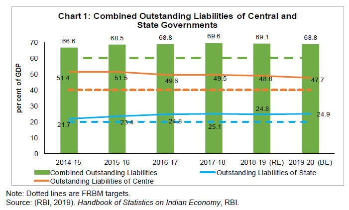 Analysing the growth of outstanding liabilities of the Centre and the growth of GDP (nominal), one sees that GDP growth has mostly been higher than growth in liabilities, thus explaining the declining trend of the outstanding liabilities as percent to GDP (Chart 2). Also, interest payments to revenue receipts, an indicator of debt servicing, have remained contained for the Centre. 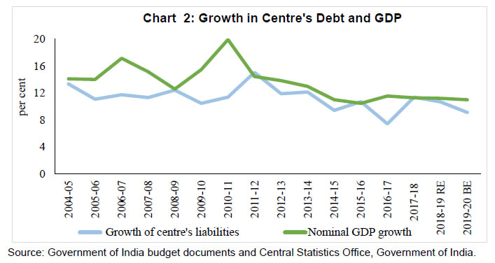 For the states, debt is increasing at a double-digit rate, at a pace higher than nominal GDP growth (Table 1). States’ debt rose for about a decade prior to 2003–04, but witnessed a significant consolidation after the enactment of FRLs by the states. The adherence to the fiscal rule legislations was also supported by the debt relief provided by the two debt restructuring schemes, viz. Debt Swap Scheme which was in operation from 2002–03 to 2004–05 and Debt Consolidation and Relief Facility which was functional during the Twelfth Finance Commission (FC-XII) award period 2005–06 to 2009–10. As a result, the ratio of interest payment to revenue receipts declined sharply during the period 2003–04 to 2014–15. However, after the implementation of the UDAY scheme, states’ debt recorded a sharp increase in 2015–16 and 2016–17 to around 25 per cent of GDP. The expenditure pressures on account of large committed expenditures and schemes like farm loan waivers also contributed to the recent rise in states’ debt (Table 1 and Chart 3). Another indicator—debt to own revenue receipts ratio—of state governments reversed its declining trend in the post-UDAY period, crossing 300 per cent since 2015–16 (Chart 4). 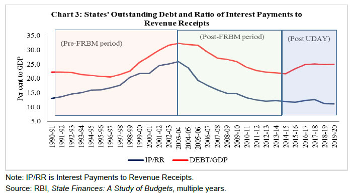 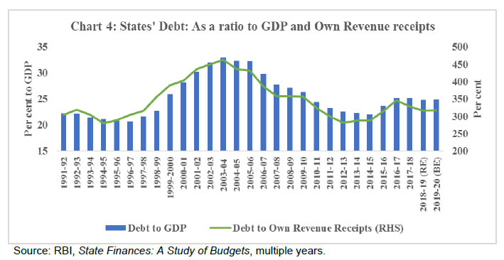 A scatter plot depicts a positive relationship between fiscal deficit and debt. As per the 2018–19 Revised Estimates (RE) data, many states remain below the 3 per cent ratio of fiscal deficit to GDP, while the threshold debt to GSDP ratio of 25 per cent as perceived by the Fourteenth Finance Commission (FC-XIV) stands breached by many states. However, if we consider a little strict measure of the implicit FRBM debt ceiling of 20 per cent prescribed by the FRBM Review Panel (as adopted in the Union Budget 2018–19), most states remain above the threshold level (Chart 5). 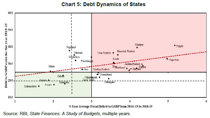 On comparing India’s subnational debt vis-à-vis that of its BRICS6 counterparts, India’s debt remains the highest (Chart 6) followed by China. China’s official debt has accumulated largely due to rising local government debt and the subdued performance of public sector enterprises (PSEs). In addition, if the off-budget liabilities of local government amounting to 30 per cent of GDP are added, then subnational debt for China would rise to over 50 per cent in 2017 (IMF, 2018). Other countries’ debt, e.g. Colombia, Argentina, and Indonesia, featuring market borrowings by states, remained subdued and amounted to less than 10 per cent of their GDP. 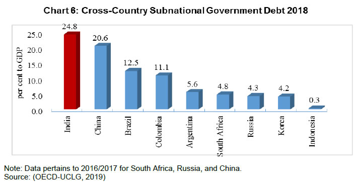 Going Beyond State Governments’ Conventional Debt — Guarantees Apart from direct budgetary support to SPSEs, through equity and loans, state governments provide off-budget support to SPSEs by providing guarantees on repayment of their borrowings taken from financial institutions and share of such off-budget borrowings has gone up in recent years. This has linkages both with the institutional structure of the fiscal framework for the Centre–state relationship and the need for strict adherence to the fiscal rules on the part of states amidst the rising responsibilities entrusted on them. Fiscal consolidation at the subnational level in India has been undertaken under a rule-based framework through the enactment of FRLs by states in the early 2000s. The immediate post-FRL period saw large-scale improvement in fiscal performance. While high economic growth could have influenced states’ revenues in a positive way, one also observes focused expenditure rationalisation measures undertaken by states in the post-FRL period: states increased the age of retirement, introduced voluntary retirement schemes, imposed restrictions on new recruitments, and tweaked discount rates for commutation of pensions. The successful implementation of value-added tax (VAT) by states/union territories (UTs) reflected their commitment towards revenue augmentation. Unlike the immediate post-FRL period, when fiscal consolidation was supported by a rise in receipts coupled with a fall in expenditure, the current decade, particularly post 2013, has been marked by a rise in expenditure at a rate higher than that of the rise in revenue receipts for states (Chart 7). Furthermore, an increase in total expenditure is primarily on the revenue expenditure front, mostly non-developmental expenditure, primarily wages and salaries and other committed expenditures in the form of pension payments, administrative services and, lately, interest payments. 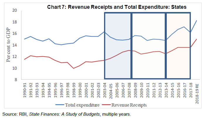 The states took recourse to curtail capital expenditure to meet fiscal targets amidst the rise in revenue expenditures, thus deteriorating the quality of the expenditure. There are also instances of pushing the capital expenditures to SPSEs by giving them guarantees with a concomitant rise in off-balance-sheet expenditures (CAG, 2019). The support through guarantees is driven by the necessity to meet the requirements of financing infrastructure with the limited fiscal space available to the states. Accordingly, while budgetary support to the SPSEs to meet their capital requirements saw a gradual decline, issuance of guarantees by state governments helped these entities to borrow from the market.7 These guarantees help states to undertake capital expenditure in key infrastructure sectors like utilities, transportation, etc. Operating through SPSEs also helps states achieve some of their macroeconomic goals, particularly in sectors characterised by market failures. However, conducting capital expenditure through SPSEs with the use of guarantees, while desirable, has been fraught with challenges for state entities. The weak cost recovery mechanisms very often make them a source of fiscal risk for state budgets (ECB, 2011; Twelfth Finance Commission, 2005), either implicitly through repayments or explicitly through the takeover of outstanding debt. The poor financial performance and weak balance sheets of the SPSEs increase the vulnerability of state governments towards the invocation of guarantees, a frequent occurrence in the past under schemes like OTS, FRP, and UDAY. Against this background, this paper explores the concept of augmented debt by incorporating outstanding guarantees, essentially a part of contingent liabilities, to assess the debt positions of state governments. Certain institutional mechanisms are put in place to safeguard against the excessive reliance of SPSEs on guarantees and any likely invocations. States impose a guarantee fee, which varies from 0.5 per cent to 2.0 per cent of guarantees issued, depending upon the quality of the borrower and states’ fiscal stance, though very often these are waived off. The optimal or sustainable level of such guarantees is based on annual incremental guarantees as a ratio to GSDP or total revenue receipts specified in the various states’ Government Guarantees Acts or fiscal responsibility legislations (FRLs) of states; otherwise administrative limits are fixed, albeit not all states have such caps/limits. States are required to set up the Guarantee Redemption Fund (GRF) with the Reserve Bank using the guarantee fees. It is supposed to be used to make payments emanating from guarantees issued on behalf of state-level bodies as per the Twelfth Finance Commission (FC-XII) recommendation (RBI, 2019). As of May 1, 2018, this rule is adhered to only by 12 states, which have established their GRF. Moreover, states like Punjab have zero balance in its GRF and some others have inadequate funds. On an aggregate basis, corpus in GRF hovers at less than 1.5 per cent of outstanding guarantees indicating small buffers if crystallisation of guarantees takes place. Needless to say, there are differences amongst states in terms of awareness about fiscal risk associated with the issuance of these guarantees and putting an appropriate mechanism in place to minimise the spillover effect onto state budgets from guarantees (see Appendix Table A1). Nevertheless, the information base on state governments’ guarantees is very weak as data on guarantees are generally not reported explicitly by state governments in their budget documents. The Comptroller and Auditor General (CAG) of India, through its state-wise report of state government finances, releases data on guarantees, though there is a lag of two years in the reporting of the same. Against this backdrop, the following analysis relies on historical data from these reports and is supplemented with data obtained from RBI’s annual publication of state finances.8 The outstanding guarantees of states witnessed a declining trend in the post-FRBM period, plummeting from 5.4 per cent of GDP at end-March 2006 to 2.0 per cent of GDP at end-March 2017 (Table 2). The decline in guarantees is primarily driven by the guarantees of the power sector being subsumed in state government liabilities under UDAY, which is typically reflected in the corresponding rise in debt levels of state governments. However, in 2017–18, guarantees witnessed a significant jump to 2.5 per cent of GDP (year-on-year growth of about 38 per cent), indicating early signs of fiscal risks (Chart 8).9 Likewise, the augmented debt, which is the sum of conventional debt and guarantees, has recorded a rise and stood close to 28 per cent at end-March 2018. 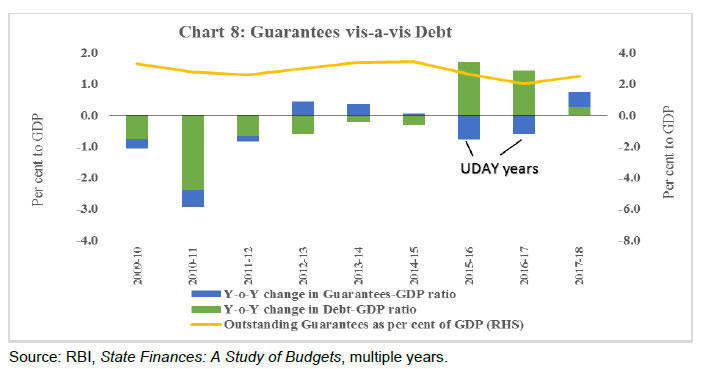 In terms of sectoral distribution, guarantees provided to power utilities remain dominant—greater than 60 per cent (on average) of total outstanding guarantees. For a few states like Rajasthan, Uttar Pradesh, Tamil Nadu, Meghalaya, Manipur and, Himachal Pradesh, guarantees taken by the power sector account for over 80 per cent of total guarantees followed by the transport sector (Chart 9). 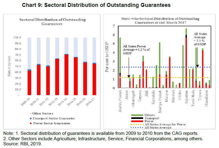 It is worthwhile to note that the extent and growth of guarantees vary widely across states. States like Rajasthan, Uttar Pradesh, Andhra Pradesh, and Kerala have a high incidence of guarantees (as defined by guarantees to GSDP ratio), while Gujarat, Odisha, and Uttarakhand have a low incidence of guarantees with low/no growth. However, some states like Maharashtra, Bihar, and Karnataka currently have a relatively small incidence of guarantees, but are experiencing significant growth in the recent period indicating potential fiscal risks in the future (Chart 10). Furthermore, most of the SPSEs have incurred significant losses, reflecting poor debt servicing capacity and the likely fall of these guarantees on the state governments going forward. 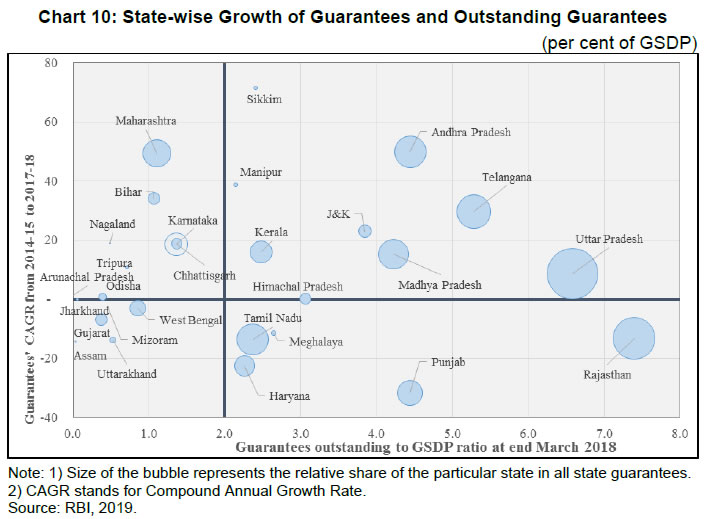 On close examination of UDAY, which led to a significant increase in states’ outstanding debt, if a part of the guarantees is invoked in the future, the consequent financial burden may fall on states’ budgets. As a result, states may have to resort to its financing via borrowings like UDAY bonds with macro implications. Accordingly, an alternate variable has been considered in the empirical analysis along with debt, which is the augmented debt (debt plus guarantees), to explore whether states’ debt is sustainable or not if the guarantees are invoked. III. Theoretical Underpinnings and a Review of the Literature Theoretical Literature Review Debt, by definition, is considered to be sustainable if a country is expected to service its debt without any large future corrections in the primary balances of the government. It rules out a situation where the borrower accumulates debt faster than its capacity to service the existing debt, known as Ponzi finance (Blanchard et al., 1990; Buiter et al., 1985). Other definitions, particularly post-crisis, by the International Monetary Fund (IMF) and others focus on the serviceability of debt, i.e. the sustainable debt of a country suggests its ability to service all accumulated debt at any point in time (IMF, 2011). Typically, debt sustainability can be explained using an accounting-based approach associated with an inter-temporal budget constraint as shown below: 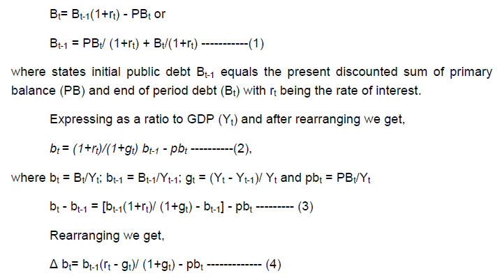 The condition for debt sustainability is to place the debt on a stable or declining trajectory which specifies Δ bt < 0, as per equation 4.10 Fiscal policy is thus unsustainable when gt = rt and gt < rt as debt grows linearly in the case of the former and explosively in the case of the latter. Debt is sustainable when gt > rt. This is considered to be one of the necessary conditions for sustainability (in line with Domar, 1944). The other condition is that the primary balance (pb) has to be positive and large. However, Δ bt < 0, this condition can be achieved even with primary deficits (pb<0) if the same is offset by a sufficiently large negative interest-growth differential (rt - gt). Since the government in emerging economies, including India, usually run primary deficits, they are dependent on a negative interest-growth differential to contain the debt-GDP ratio. It follows that, if India were not able to maintain its growth rate and if interest rates start rising, then the country’s debt-GDP ratio could begin to spiral upwards. For advanced economies, the interest-growth differential is usually close to zero; further, this differential should not exist in the long run, as is advocated by growth theories. Thus, if rt - gt is zero, then the primary balance must also be zero or in surplus to satisfy the condition for debt to be sustainable. These are some of the theoretical underpinnings which are utilised to assess debt sustainability in the following standard frameworks. Empirical Literature Review In the empirical framework, the concept of debt sustainability is primarily measured by two approaches: (i) using the indicators of debt sustainability (Blanchard, 1990; Buiter et al., 1985, 1987; Buiter et al., 1993; Miller, 1983), and (ii) through the model-based approach using econometric methods of government solvency (Bohn 1998; Hamilton and Glavin 1986; Trehan and Walsh 1988). The existing literature does not consider one approach to be better than the other; however, it does suggest an integration of the results from these two approaches in order to provide additional information on the aspect of debt sustainability (Marini and Piergallini, 2008). The indicator-based approach evaluates the creditworthiness of the borrower with the help of indicators as derived from the inter-temporal budget constraint (equation 4 above), viz. (a) whether the real rate of interest minus real GDP growth is negative and/or (b) whether there is a primary surplus or deficit. This approach has been further extended by adding more indicators that reflect growth, liquidity, and serviceability of debt such as the ratio of interest payment to current revenue, the difference between the rate of growth of debt, and the rate of growth of nominal GDP, among others. While some of the early papers on debt sustainability for India have used this approach exclusively, the latest ones have used it along with other approaches (Dholakia et al., 2004; Kaur et al., 2018; Mishra and Khundrakpam, 2009; Mourya, 2015; Pattnaik, et al., 2003; Rajaraman et al., 2005). While the indicator-based approach is largely forward-looking, albeit static, the empirical technique using an econometric model based on historical time-series data is considered largely backward-looking, though dynamic by nature. The model-based approach has also different variants that have evolved over time. The unit root test was used extensively to check debt sustainability in the United States (US), first by Hamilton and Flavin (1986) and later by Trehan and Walsh (1988), who used it along with the cointegration approach. In the Indian case, studies by Buiter and Patel (1992) and Pradhan (2014) used the unit root approach, while Jha and Sharma (2004) and Tronzano (2013) relied on the cointegration approach. Given the limitations of the aforementioned model-based approaches, the Bohn approach, which estimates the fiscal policy response function, emerged as an alternative and has been extensively used to assess the sustainability of public debt policies amongst different countries (Ostry and Abiad, 2005; Adam et al., 2010; Greiner and Kauermann 2008; Haber and Neck, 2006; Kaur et al., 2018; Renjith and Shanmugam, 2018). The economic intuition behind the Bohn approach is: If governments run debt today, how will primary balances be impacted to assess whether public debt is sustainable or not? Amongst the international studies, Greiner and Kauermann (2008) analyse this issue by performing the spline smoothing technique and time-varying coefficients for Germany and Italy. The analysis reveals evidence of a sustainable debt in Germany with a declining tendency, while Italy’s debt was not found to be sustainable. Contrasting this, using the wavelet analysis and a longish time-series analysis of around a decade and a half for Italy, the presence of enduring debt sustainability was found (Magazzino and Mutascu, 2019). A panel estimation study by Adams et al. (2010), which combined countries of Central Asia, East Asia, the Pacific, Southeast Asia, and South Asia for a relatively small period, indicated public finances of developing Asia to be in good shape. Many studies have used this approach to explore the issue of debt sustainability either in a panel framework or time series; however, results are subject to the underlying assumptions and analytical techniques used to perform the analysis. In the context of India, while studies have conventionally analysed debt sustainability for the Centre and general government (Centre plus states) (Hakhu, 2015; Mohanty and Panda, 2019; Rajaraman and Mukhopadhaya, 2004; Rangarajan et al., 1989; Seshan, 1987) and both for domestic and external debt (Cashin and Olekalns, 2000), the existing empirical literature on states’ debt sustainability remains sparse with mixed results. Early studies by Tiwari (2012) and Misra and Khundrakpam (2009) which cover the initial years of the post-FRBM period when the debt was at a relatively higher level found evidence of debt unsustainability in the long run, while studies such as Renjith and Shanmugam (2018) and Kaur et al. (2018) covering the later time period observed debt to be sustainable. Regardless of the time period, results amongst studies vary on based on the estimation method adopted. Summary results of select empirical studies dealing with this research question are presented in Table 3. A review of the Indian literature available on public debt sustainability clearly reveals that most studies on the subject have limited their analyses to conventional debt sustainability and have not assessed the potential risks from contingent liability realisations. Given the fact that a significant portion of the guarantees accrues to the financially underperforming state power sector utilities, the prospects of their crystallisation are higher and therefore the consequent financial burden may fall on states’ budgets. It should be noted that this issue has been highlighted by other studies as a potential research gap (ECB, 2011; Kaur et al., 2018).11 Contingent liability realisations have been ascribed to be a more important cause than an addition to the primary deficit behind debt spikes across countries (Jaramillo et al., 2017). Against this backdrop, this study attempts to address this research gap specifically in the Indian context by including the post-UDAY period (2015–17) when debt swelled up sizeably; incorporating a larger number of states, thereby improving spatial coverage vis-à-vis existing studies; and, lastly, by adding the contingent liabilities in the form of state government guarantees into the conventional debt analysis. Methodology On the basis of the foregoing literature review, the objective of this study is to analyse the debt sustainability of state governments. Towards this endeavour, the empirical analysis in this paper is based on three stages. First, a forward-looking indicators-based approach is used to provide a quick assessment of the ability of state governments to service as well as to repay their debts through current and regular sources of income.12 Second, the order of integration of all the variables is checked using panel unit root tests. Third, the fiscal policy response function for state governments is estimated in a panel framework using a standardised Bohn approach (Bohn, 1998). The indicator-based approach considers the creditworthiness of the borrower by analysing ratios. As per the necessary Domar stability condition, the real growth rate of the economy should be higher than the real interest rate, while the sufficient condition states that primary balances should be zero or in surplus to service the future debt (drawing from equation 4). Along with these debt servicing indicators, the ratio of interest payment to revenue receipts should be declining and less than 10 per cent (Fourteenth Finance Commission [FC-XIV]) and debt should be growing at a rate lower than GDP growth for it to be sustainable. Fiscal Policy Response Function (Bohn Approach) A basic fiscal policy response function adopted from the Bohn approach can be illustrated as follows: 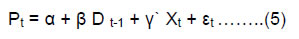 where P is the primary balance-to-GDP in year t; D t-1 is debt stock in t-113 and X denotes control variables, viz. real GDP gap, revenue receipts, primary expenditure, etc. ‘β’ is the principal coefficient which measures the response of the primary balance to variations in debt. If a rising debt-to-GDP ratio leads to a rise in primary balance, then debt tends to be sustainable. Equation (5) has been estimated using a fixed-effect model and/or random-effects model. The former allows for all unobserved factors (varying across states though remaining constant over time) to be correlated with the explanatory variables, while the latter assumes that they are uncorrelated with the explanatory variables and so are included in the error term (Gupta and Ahmed, 2018). The Hausman specification test has been applied to decide upon the fixed effects/random effects model wherein the null says there is no significant difference between these two estimations.14 In addition, regressions are carried out with Feasible Generalised Least Squares (FGLS) to further check the robustness of empirical results (Ostry and Abiad, 2005; Adams et al., 2010Ostry and Abiad). The classic OLS regression assumes independent identically distributed (i.i.d) error and independent autocorrelation structure. But in many cross-sectional data sets, the variance for each of the panels differs. Recognising that this study uses data from heterogeneous states that may have variations of scale, ruling out heteroscedasticity could be important. This problem of heteroscedasticity can be countered if the variance-covariance matrix of the error term is known. There are typically two ways to address this issue. One can either (a) assume the structure of the variance-covariance matrix which is known as weighted least squares (WLS) estimation or/and (b) estimate it empirically from ordinary least squares (OLS) rather than assuming, referred to as FGLS estimation. Furthermore, FGLS estimation has an advantage that it can also correct for cross-sectional correlation and autocorrelation, if any occurs (Greene, 2012). Data The data used in this study to carry out the empirical analysis are described in this section. We have considered annual time series from 1992–92 to 2018–19 to perform the indicator-based analysis for all states, while a panel analysis is conducted for the period 2004–05 to 2017–1815 for 26 states. The choice of states and time period in the panel data has been determined by the availability of guarantees data, though we have tried to remain as comprehensive as possible. Since data points for the variable outstanding guarantees were not available for two states, viz. Goa, and Jharkhand, augmented debt could not be obtained. Also, with the Telangana region being merged with Andhra Pradesh, few data points were available for Telangana’s guarantees data. Consequently, 26 states are considered over a period of 14 years. As debt stock is taken with a lag of one year, the number of observations in this analysis is 338 (26×13). Data on various fiscal variables are extracted from State Finances: A Study of Budgets of 2019–20, an annual publication of the RBI, while state-wise GSDP (real and nominal) is from the Ministry of Statistics and Programme Implementation (MoSPI). We have used two specifications of the standard fiscal policy response function, discussed below: 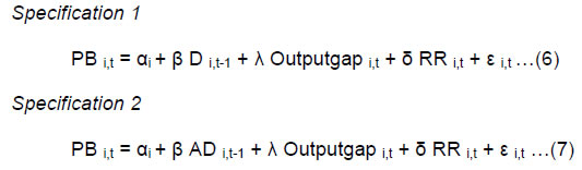 where PB represents primary balance to GSDP ratio; D is debt to GSDP ratio; Output gap signifies the difference between the real output and the potential real output; RR represents revenue receipts to GSDP ratio; ε is error term; and AD is augmented debt to GSDP ratio. This study analyses two variants of the principal explanatory variable debt wherein Specification 1 (equation 6) assesses the sustainability of conventional debt “D”, while Specification 2 (equation 7) is beyond estimating conventional debt sustainability and so incorporates off-budget liabilities in the form of outstanding guarantees issued to SPSEs. This new principal variable is referred to as augmented debt “AD” in this study. Further, under Specification 2, two scenarios are considered. In the first scenario, all guarantees are added to the conventional debt, while the second is based on the realistic assumption of only power sector (constituting around 70 per cent) guarantees getting crystallised. This is likely from both precedence and performance point of view. During the last 13 years, on three occasions, the Government has tried to support power sector SPSEs. Under UDAY, almost the majority of power sector debt was added to states’ debt and the impact is still being felt by many (RBI, 2019). In terms of performance, most of them are still running losses, with talk of another restructuring required. In such a situation, it would be prudent to add the power sector guarantees to conventional debt in order to arrive at the augmented debt and to highlight fiscal risks. While the first scenario represents an extreme situation—as not all guarantees will be invoked at the same time—keeping this scenario helps to understand the maximum fiscal risks posed by these off-budget liabilities. This is important in the context of the global debate on adopting a public sector balance sheet approach (IMF, 2018) and also considering the fact that some Latin American countries have started including state-owned enterprises in their fiscal targets. The coefficient “β” is the key to estimating the response of primary balance to debt as per Specification 1 and, likewise, augmented debt as per Specification 2. A positive coefficient lying between zero and one depicts the sustainability of public debt. While a negative β coefficient indicates the unsustainability of public debt. Two control variables, namely the real output gap and revenue receipts (RR), are employed in line with Ostry and Abiad (2005). The real output gap is measured as the difference between the actual real GSDP and the potential real GSDP wherein the latter is estimated using the Hodrick–Prescott (HP) filter. A positive coefficient of the output gap (actual output is above the potential output) indicates that primary balance improves when real GSDP is above the potential and therefore surplus rises in response to cyclical effects on revenues and expenditures. The other control variable RR allows us to distinguish fiscal structures amongst states. Given the weak revenue-raising capacity amongst the majority of Indian states, more so after the implementation of GST, the use of revenue receipts to GSDP can be considered as a direct proxy for states’ surplus generating capacity, particularly considering that few states have higher revenue-generating capacities than others. Hence, RR is illustrative of robust fiscal capability. Furthermore, to underpin the empirical results, we conducted a robustness check by using the revenue receipts gap and the average of RR to GSDP ratio over the previous two years, rather than contemporaneous revenue receipts to GSDP ratio. Further, the other control variable—primary expenditure gap—which is the difference between the actual primary expenditure16 and the trend primary expenditure capturing deviations in primary expenditure from long-term trend, is also considered. Higher primary expenditure from the trend signifies deterioration in primary balance. Indicator-based Approach A quick assessment of the ability of state governments to service and repay the debt through current sources of income is conducted using an indicator-based approach. By dividing the entire post-reform period 1992–93 to 2018–19 into different phases based on the fiscal performance of states and by analysing the debt sustainability indicators of all the states together, we found that the real rate of interest is lower than the real GDP growth rate in all phases, thus fulfilling the necessary condition for debt sustainability (Table 4).17 However, the GDP growth-interest rate differential has narrowed down in the last five years, necessitating the need for larger and faster corrections in primary deficits for debt to be in a sustainable path (Chart 11). Furthermore, the primary balance has remained consistently negative (implying primary deficits) throughout all phases (except Phase III), consequently violating the sufficient condition of debt sustainability (Table 4). The last phase (2015–16 to 2018–19), coinciding with the issuance of UDAY bonds, witnessed the highest primary deficit in the post-FRBM period. The declining (r-g) coupled with a rising primary deficit hint at the fast-shrinking window for debt sustainability. The next indicator, i.e. interest payments to revenue receipts ratio, is essentially a debt servicing indicator reflecting how much of the revenue receipts go towards financing interest payments. Notwithstanding a decline in this ratio over the phases, the ratio is still higher than the tolerable limit of 10 per cent as prescribed by the Fourteenth Finance Commission (FC-XIV). Lastly, while debt was growing at a rate lower than the nominal GDP growth in the post-FRL phases, in the latest post-UDAY phase, the rate of growth of debt stood higher than the growth rate of nominal output signalling potential debt sustainability risks. The ambivalence in this indicator-based approach of debt sustainability demands further investigation of the solvency of state governments. A quick comparison with previous such analysis (Kaur et al., 2018) reveals deterioration in most of the indicators in the latest phase (Phase VI), which primarily looks to be a fallout of realisations of contingent liabilities under UDAY. 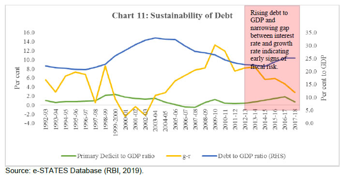 Model-based Econometric Approach Before opting for the panel regression approach, we investigated the time-series properties of all the variables, viz. primary balance to GDP ratio, debt to GDP ratio, augmented debt to GDP ratio, real output gap, and revenue receipts. Different methods of panel unit root tests were applied in our investigation. The Levin, Lin and Chu (LLC) panel unit root test assumes a common unit root across cross-sections, while the Im–Pesaran–Shin (IPS) and Fisher–ADF assume individual unit root processes. Here, the null signifies the presence of a unit root at level, while its rejection ascertains that the data series is stationary. The results of all the panel unit root tests are presented in Table 5, and these three tests unanimously suggest that all the variables are stationary at level. After ensuring the stationary properties of data, the fiscal policy response function is measured using the panel estimation methods. The Hausman specification test validates the random-effects model. A diagnostic check revealed the presence of heteroscedasticity, though the model did not suffer from autocorrelation and cross-section dependence of residuals, something typical of macro panels with long time series. Consequently, the FGLS model is also applied as it deals with heteroscedasticity. Empirical results of alternate models described above are summarised in Table 6.18 Model 1 (that uses random effects) gives a negative and statistically significant β coefficient at 1 per cent level, while Model 2 (that corrects for heteroscedasticity using FGLS) offers a statistically insignificant β coefficient, thus rejecting the null of unsustainability of states’ debt. These results may signify weak evidence with regard to the sustainability of states’ debt. However, with the inclusion of all guarantees (referred to as augmented debt under Scenario 1), debt clearly moves into the unsustainable path as shown under both Model 3 and Model 4. This suggests that the primary balances in India respond negatively to increases in augmented debt, indicating that the debt sustainability condition for an intertemporal budget constraint is not satisfied. We have also considered a slightly more likely Scenario 2 (see Models 5 and 6), when a part of guarantees, particularly those in the power sector, is invoked, which also further confirms the likely unsustainability of states’ debt. Thus, this paper supports the argument that primary fiscal balances of subnational governments in India respond in a destabilising manner if the debt is considered in the augmented form (inclusive of guarantees).19 The control variable (revenue receipts) is correctly positively signed and statistically significant at 1 per cent level, signifying that higher revenue generation helps to improve primary balances. This also allows to distinguish fiscal structures amongst states, as some states have higher revenue-generating capacities compared with others. Further, a positive and significant coefficient of output gap indicates that primary balances improve in response to cyclical effects, particularly due to the impact on states’ own revenues and central transfers. These empirical results are broadly robust to various alternative specifications, as provided in Appendix Table A2. Alternate specifications are based on different control variables such as revenue receipts gap, primary expenditure gap and average revenue receipts with debt and augmented debt (obtained by adding only power sector outstanding guarantees, about 70 per cent of the total, to outstanding liabilities, which is a more likely scenario) as prime independent variables under both RE and FGLS model specifications. It is observed that broadly the sign and significance of debt and augmented debt are retained. In general, as we move from debt to augmented debt liabilities, the β coefficient indicates that debt moves from sustainable to unsustainable ranges or, if already unsustainable, the strength and significance of the coefficient increases. In the case of a control variable, the output gap loses its significance. These results are robust to the inclusion of time and fixed effects in the regression. These robustness checks further buttress the empirical results of this study and hence reconfirm the augmented debt unsustainability concerns of the states in the long run. VI. Conclusion and Policy Implications The debt position of state governments, after remaining in the comfort zone for about a decade post-FRL, has started showing early signs of unsustainability in the post-UDAY period. Apart from the conventional liabilities of state governments, fiscal costs can also stem from state governments’ risk exposure to their public sector in the form of guarantees, off-budget borrowings, and accumulated losses of financially distressed PSEs. The empirical analysis of debt sustainability in this paper, using both indicators as well as Bohn’s (1998) panel data approach, indicates that guarantees given by states, if invoked, can turn out to be a potential risk to debt sustainability for the Indian states. With regard to policy implications on the fiscal side, it may be pertinent to review the FRL adopted by the states in the 2000s, much the same way the Centre revised their FRBM in the 2018–19 Union Budget whereby debt was explicitly added as a target variable along with fiscal deficit. This is particularly desirable considering the fact that while the fiscal deficit of states remains well within their FRL threshold of 3 per cent for GFD to GDP ratio, as adopted during the early 2000s, the debt is rising at a high pace, crossing corresponding implicit thresholds. Besides, no fiscal rule is static and the cross-country evidence suggests that fiscal rules may entail improvisation contingent upon experience. Laying down a transparent institutional mechanism may ensure that states meet their debt-deficit targets. In the context of the SPSEs, it may be important to: (i) periodically review the performance of SPSEs to examine whether they can deliver value for the taxpayer’s money (IMF, 2018); (ii) get their pricing policy right so that they are able to ensure cost recovery through appropriate user charges/tariffs, etc. (RBI, 2019); and (iii) ensure professional and transparent operation of these units. Measures must be adopted to ensure a comprehensive framework for guarantees management which would include elements like adherence to caps/limits based on sustainability; providing transparent data on guarantees extended by states and the consequent invoking/ waiving off of unpaid subsidies20, if any, by the state governments; and, charging guarantee fees to avoid any kind of moral hazard on the one hand, and also to add to revenues of the states, on the other. @Sangita Misra (sangitamisra@rbi.org.in) and Kirti Gupta (kirtigupta1@rbi.org.in) are Director and Manager (Research), respectively, in the Department of Economic and Policy Research (DEPR), Reserve Bank of India (RBI); Pushpa Trivedi (trivedi@hss.iitb.ac.in) is Professor and Head, Humanities and Social Sciences, Indian Institute of Technology Bombay. *The authors are thankful to: Prof. Ganesh Kumar, Indira Gandhi Institute of Development Research (IGIDR) and Shri S. Suraj, RBI, who discussed the paper and offered their comments in the DEPR Study Circle; Atri Mukherjee, Director, DEPR, RBI, for her valuable suggestions on an earlier version of the paper. The views expressed in the paper are those of the authors and not the institutions to which they belong. The usual disclaimer applies. 1 States’ market borrowings have more than doubled in the last 5 years. 2 Under the OTS of 2003, the outstanding dues of the State Electricity Boards to the central public sector undertakings (PSUs) were taken over by the state governments through the issuance of power bonds (with SLR status) amounting to ₹29,606 crores. The FRP 2012 restructured the debt of state power distribution companies (DISCOMs) by taking over 50 per cent of their outstanding short-term debt obligations up to March 31, 2012. This increased state governments’ outstanding guarantees in 2012–13 and 2013–14 since seven states, viz. Andhra Pradesh, Punjab, Rajasthan, Uttar Pradesh, Haryana, Tamil Nadu, and Bihar guaranteed the issuance of bonds by DISCOMs to their lenders. UDAY, which covered all states/union territories except West Bengal, Odisha, and Delhi, was conceptualised in 2015 as a comprehensive measure to turn around the state-owned distribution utilities both operationally and financially. The states took over 75 per cent of the DISCOMs’ debt, which amounted to ₹2.1 lakh crore, through the issuance of non-SLR UDAY bonds and transferred the proceeds to DISCOMs. A total of 16 states who adopted comprehensive financial and operational agreements issued bonds under UDAY in 2015–16 and 2016–17, leading to a sharp rise in these states’ debt, interest payments and redemption pressures. 3 This study does not go beyond 2017–18 primarily for two reasons. First, the years 2018–19 and 2019–20 do not represent actuals; they represent revised and budget estimates, respectively. A vast discrepancy has been observed between actuals and revised/budgeted estimates of state finances (RBI, State Finances: A Study of Budgets, multiple years). Therefore, in order to avoid this discrepancy, the period of study is limited till 2017–18, representing only actuals. Second, this study aims to compare conventional debt with augmented debt and due to data constraints on guarantees, our analysis has been restricted until 2017–18. 4 Since the Fourteenth Finance Commission (FC-XIV) found the differentiation between special category state and non-special category state redundant, we have considered all states in our study. 5 In this study, subnational debt refers to the debt of the state governments only, local bodies’ debt is not included due to its unavailability. 6 BRICS is the acronym coined for an association of five major emerging national economies: Brazil, Russia, India, China, and South Africa. 7 Article 293 of the Indian Constitution puts a restriction on overall borrowings by states that are sanctioned by the Centre till the time the previous loan provided by the central government is outstanding. Additionally, SPSEs are allowed to raise off-budget borrowings along with guarantees which are provided by states under Article 293 (1) of the Constitution. 8 A state-wise time series on guarantees outstanding can be culled out from RBI’s annual publication State Finances: A Study of Budgets of 2019–20 (RBI, 2019) under Statement 28. 9 At end-March 2019, guarantees’ data are available for only 11 states and amounted to 0.8 per cent of GDP. Using the same states’ data for the previous year, outstanding guarantees amounted to 0.6 per cent of GDP, clearly exhibiting a rise in guarantees issued in 2018–19. 10 In practise, equation (4) can also be modified to Δ bt = bt-1(rt - gt)/ (1 + gt) - pbt + ddatwhere ddat refers to deficit-debt adjustment as a share of GDP comprising factors that affect debt but are not included in budget balance (Bouabdullah et al., 2017; Jaramillo et al., 2017). With ddat = 0, stability conditions as stated above remain the same. 11 It may be noted that Buiter and Patel (1992) is the only previous study that has assessed the debt sustainability for Centre, states, and PSUs together. It finds the discounted debt series—using various alternative measures of interest rates—to be non-stationary and hence unsustainable. The study though remains significantly dated. 12 The current sources of revenue should not include any temporary revenues/grants or capital receipts emanating from the sale of assets. 13 To avoid the endogeneity issue, Dt is replaced by Dt-1. 14 The P-value of chi-square statistic being greater than 5 per cent, any deviation is due to chance alone 5 per cent of the time or less and hence the random effect model is appropriate. 15 Footnote 4 explains why the panel analysis conducted does not go beyond 2017–18. 16 Primary Expenditure = Total Expenditure - Interest Payments. 17 The phase-wise break-up is based on trends in key fiscal parameters. After improving slightly during the immediate post-reform period (1992–93 to 1996–97: Phase I), fiscal parameters deteriorated sharply during Phase II. With the adoption of FRLs in 2003–05, fiscal indicators improved significantly (Phase III) until the crisis in 2008–09. The immediate post-crisis period (Phase IV) was marked by deterioration in fiscal and primary deficit led by fiscal stimulus measures, albeit debt continued its declining trend. During Phase V, the pace of decline in debt slowed down, and, finally, in Phase VI, debt has started rising with the issuance of UDAY bonds and poor performance of SPSEs. 18 While FGLS is asymptotically more efficient than OLS for a large sample, for a small/medium-sized sample it can be less efficient than OLS, although coefficients are unbiased allowing for heteroscedasticity and autocorrelation. So, it is better to present both OLS and FGLS. FGLS might also be inconsistent if there are individual specific fixed effects, although, in this case, that is ruled out through the Hausman test. 19 Though different from Kaur et al. (2018), who observe states’ debt to be sustainable, the results are not strictly comparable given the broader debt definition used in the paper with expanded spatial and temporal coverage for states. 20 Because arrears on subsidy are not captured in state budgets since the budgets follow cash accounting as opposed to accrual-based accounting. References Adams, C., Ferrarini, B., & Park, D. (2010). Fiscal sustainability in developing Asia. ADB Economics Working Paper Series, No. 205. Blanchard, O. J. (1990). Suggestions for a new set of fiscal indicators. OECD Economics Department Working Paper No. 79. Blanchard, O., Chouraqui, J. C., Hagemann, R.P., & Sartor, N. (1990). The sustainability of fiscal policy: New answers to old questions. OECD Economic Studies, No. 15. Bohn, H. (1998). The behavior of U.S. public debt and deficits. Quarterly Journal of Economics, 113, 949–963. Bouabdullah O., Westphal, C. C., Warmedinger, T., de Stefani, Roberta, Drudi, F., Setzer, R., & Westphal, A. (2017). Debt sustainability analysis for Euro Area Sovereigns: A methodological Framework. ECB Occasional Paper No. 185, April. Buiter, W. H,, T. Persson & P. Minford, (1985). A Guide to public sector debt and deficits. Economic Policy, 1(1), 13–79 —. (1987). The current global economic situation, outlook and policy options, with special emphasis on fiscal policy issues. CEPR Discussion Papers No. 210, CEPR Discussion Papers. Buiter, W. H., Corsetti, G., & Rubini, N. (1993). Excessive deficits: Sense and nonsense in the Treaty of Maastricht. Economic Policy, 8(16), 57–100 Buiter, W. H., & Patel, U. R. (1992). Debt, deficits and inflation: An application to the public finances of India. Journal of Public Economics, 47(2), 171–205. Cashin, P. & Olekalns, N. (2000). An examination of the sustainability of Indian fiscal policy. Department of Economics - Working Papers Series No. 748, The University of Melbourne. Chakraborty, P., & Dash, B. B (2017). Fiscal reforms, fiscal rule, and development spending: How Indian states have performed. Public Budgeting & Finance, 37(4), 111–133. Comptroller and Auditor General (CAG) (2019). Report of the Comptroller and Auditor General of India on compliance of the Fiscal Responsibility and Budget Management Act, 2003 for the year 2016–17, Report No. 20 of 2018, January, Union Government (Civil), Department of Economic Affairs (Ministry of Finance). Available at: https://cag.gov.in/sites/default/files/audit_report_files/ Report_No_20_of_2018_Compliance_of_the_Fiscal_Responsibility_ and_Budget_Management_Act_2003_Department_of_Economic_Affairs_Minis.pdf. Dholakia, R. H., Mohan, T. T. R., & Karan, N. (2004). Fiscal sustainability of debt of states. Study sponsored by the Twelfth Finance Commission, New Delhi. Domar, Evsey D. (1944). The "burden of the debt" and the national income. American Economic Review, 34(4), 798–827 European Central Bank (ECB). (2011). Ensuring fiscal sustainability in the euro area. Monthly Bulletin, April, ECB, Frankfurt am Main. Available at: https://www.ecb.europa.eu/pub/pdf/mobu/mb201104en.pdf. Fourteenth Finance Commission. (2015). Report of the Fourteenth Finance Commission. Ministry of Finance. Greene, W. H. (2012). Econometric analysis (7th ed.). Upper Saddle River, NJ: Prentice Hall. Greiner, A., & Kauermann, G. (2008). Debt policy in euro area countries: Evidence for Germany and Italy using penalized spline smoothing. Economic Modelling, 25(6): 1144–1154. Gupta, K., & Ahmed, S. (2018). Determinants of FDI in South Asia: Does corruption matter? International Journal of Economics and Business Research, 16(2), 137–161. Haber, G., & Neck, R. (2006). Sustainability of Austrian public debt: A political economy perspective. Empirica, 33(2–3), 141–154. Hakhu, A. (2015). Productive public expenditure and debt dynamics: An error correction representation using Indian data. Working Papers No. 15/149, National Institute of Public Finance and Policy, New Delhi. Hamilton, J., & Flavin, M. A. (1986). On the limitations of government borrowing: A framework for empirical testing. American Economic Review, 76(4), 808–819. International Monetary Fund (IMF) (2011). Modernizing the framework for fiscal policy and public debt sustainability analysis. Public Information Notice No. 11/118 September 12. —. (2014). Fiscal Monitor, April 2014: Public Expenditure Reform: Making Difficult Choices, IMF Fiscal Affair Department. Available at: https://www.imf.org/en/Publications/FM/Issues/2016/12/31/Public-Expenditure-Reform-Making-Difficult-Choices-41121. —. (2018). Fiscal Monitor, October 2018: Managing Public Wealth. Available at: https://www.imf.org/en/Publications/FM/Issues/2018/10/04/fiscal-monitor-october-2018. Jaramillo, L., Mulas-Granados, C., & Kimani, E. (2017). Debt spikes and stock flow adjustments: Emerging economies in perspective. Journal of Economics and Business, 94, 1–14. Jha, R., & Sharma, A. (2004). Structural break and unit roots: A further test of the sustainability of the Indian fiscal deficits. Public Finance Review, 32(2), 220–231. Kaur, B., Mukherjee, A., & Ekka, A. P. (2018). Debt sustainability of states in India: An assessment. Indian Economic Review, 53(1–2), 93–129. Mahdavi, S. (2014). Bohn's test of fiscal sustainability of the American state governments. Southern Economic Journal, 80(4), 1028–1054. Magazzino, C., & Mutascu, M. (2019). A wavelet analysis of Italian fiscal sustainability. Economic Structures, 8(19). Marini, G., & Piergallini, A. (2008). Indicators and tests of fiscal sustainability: An integrated approach. CEIS Working Paper No. 111. Miller, M. (1983). Inflation adjusting the public sector financial deficit. In J. Kay, (Ed.), The 1982 Budget. London: Basil Blackwell. Misra, B., & Khundrakpam, J. K. (2009). Fiscal consolidation by central and state governments: The Medium Term Outlook. RBI Staff Studies. May. Mohanty, R., & Panda, S. (2019). How does public debt affect the Indian macro-economy? A structural VAR approach. National Institute of Public Finance and Policy Working Paper Series No. 250, 22 January. New Delhi. Mourya, N. K. (2015). Debt sustainability of a sub-national government: A case study of Uttar Pradesh in India. Journal of Economic Policy and Research, 11(1), 126–146. OECD-UCLG (2019). Report on World Observatory on Subnational Government Finance and Investment. Ostry, J. D., & Abiad, A.d. (2005). Primary Surpluses and Sustainable Debt Levels in Emerging Market Countries. IMF Policy Discussion Papers, 05(6). Pattnaik, R. K., Misra, B. S., & Prakash, A. (2003). Sustainability of public debt in India: An assessment in the context of fiscal rules. In 6th Workshop on Public Finance, Bank of Italy, Italy. Pradhan, K. (2014). Is India’s public debt sustainable? South Asian Journal of Macroeconomics and Public Finance, 3(2), 241–266. Rajaraman, I., & Mukhopadhaya, A. (2004). Univariate Time-Series Analysis of Public Debt. Journal of Quantitative Economics, 2, 122–134. Rajaraman, I., Bhide, S., & Pattnaik, R. K. (2005). A study of debt sustainability at state level in India, Reserve Bank of India, Mumbai. Rangarajan C., Basu, A., & Jadhav, N. (1989). Dynamics of Interaction between government deficit and domestic debt in India. RBI Occasional Papers, September, 163–205. Reserve Bank of India (RBI) (2019). State finances: A study of budgets of 2019–20, September. —. (multiple years). State Finances: A Study of Budgets. Reserve Bank of India. Reserve Bank of India (RBI) (2019. Handbook of Statistics on Indian Economy. Reserve Bank of India, Mumbai. Renjith, P., & Shanmugam, K. (2018). Sustainable debt policies of Indian state governments. Margin: The Journal of Applied Economic Research 12(2), 224–243. Seshan, A. (1987). The burden of domestic public debt in India. RBI Occasional Papers, June, 45–77. Shastri, S., & Sehrawat, M. (2015). Fiscal policy sustainability in India: An empirical assessment. Journal of Economic Policy and Research, 10, 97–112. Tiwari, A. K. (2012). Debt sustainability in India: Empirical evidence estimating time-varying parameters. Economics Bulletin, 32(2), 1133–1141. Trehan, B., & Walsh, C. (1988). Common trends, the government's budget constraint, and revenue smoothing. Journal of Economic Dynamics and Control, 12(2–3), 425–444. Tronzano, M. (2013). The sustainability of Indian fiscal policy: A reassessment of the empirical evidence. Emerging Markets Finance and Trade, 49(Suppl. 1), 63–76. Twelfth Finance Commission (2005). Main Recommendations of the Twelfth Finance Commission. Ministry of Finance, Government of India. Von Hagen, J., & Wolff, G. B. (2006). What do deficits tell us about debt? Empirical evidence on creative accounting with fiscal rules in the EU. Journal of Banking and Finance, 30(12), 3259–3279. Appendix
| ||||||||||||||||||||||||||||||||||||||||||||||||||||||||||||||||||

شارك هذه الصفحة:


بھارت موبائل ایپلی کیشن کے ریزرو بینک کو انسٹال کریں اور تازہ ترین خبروں تک فوری رسائی حاصل کریں!
ہماری ایپ انسٹال کرنے کے لیے QR کوڈ اسکین کریں۔


صفحے پر آخری اپ ڈیٹ:


