 IST,
IST,


RBI WPS (DEPR): 11/2014: Forecasting Major Macroeconomic Variables in India - Performance Comparison of Linear, Non-linear Models and Forecast Combinations
| RBI Working Paper Series No. 11 Abstract 1 This paper adopts linear, non-linear time series models along with forecast combination (of linear and non-linear) for forecasting major macroeconomic variables (Monthly series of Index of Industrial production –IIP and quarterly series of GDP) in respect of India. It is observed that for IIP (and its sub component) series, in the short horizon (1-6 months), forecast combination (median) are found to be marginally better performing than that of linear as well as non-linear modelling framework whereas, in the long horizon (7-12 months), non-linear models perform relatively better than the linear models as well as combination forecast. For GDP (and its sub component) series, forecast combination using median forecast, has been found to be performing relatively better for both short horizon as well as long horizon. However, the paper observed improvement in forecast accuracy by using combination forecast for series with long memory property/ less volatile series. JEL Classification: E01, C01, C18, C32, C45, C49, C52, C53, C58 Keywords: Threshold Autoregressive Models, Regime Switching, Neural Network, Hurst Exponent, Rolling Forecast 1. Introduction Forecasting is an integral part of policy making for the Central bank and a robust forecasting framework is the backbone of any policy foundation. The underlying principle of any robust forecasting methodology is to identify the underlying data generating process (DGP) using various time series models. However, DGP of any macroeconomic variable undergoes changes over time due to continuous changes in macro foundation which sometimes impact the forecast accuracy adversely. Therefore, different time series techniques are used or forecasting macroeconomic variables from time to time. Linear time series techniques (like Auto Regressive Integrated Moving Average Model (ARIMA)) have been extensively used for forecasting purpose. Non-linear models started getting more focus from 1980 when researchers observed that linear models fail to identify many macroeconomic phenomenon namely asymmetric business cycles, volatility of stock exchange, inherent regime switching and many other (Tong, 1990). With the background of international experiences in application of non-linear models in forecasting arena, this paper tries to address following questions in Indian context–
The rest of the paper is organized as follows – Section 2 contains the literature review followed by methodology in Section 3, Section 4 covers the variables considered and data coverage, Section 5 provides stylish facts and Section 6 contains the empirical findings followed by conclusion. Linear time series techniques (like Auto Regressive Integrated Moving Average Model (ARIMA)) have been extensively used for forecasting purpose. Whittle (1954) observed that spectral density of AR(k) model (k determined by AIC criteria) using 660 time series observations of water level at Island Bay taken at 15 second interval indicate a significant relationship among periods of proximity peaks which cannot be explained by linear models. This was the first instance where the importance of threshold models was established. Similar phenomenon was observed by Pat (1950) in ecology. Researchers started developing various alternatives to track these non-linear features using heteroscedasticity modelling, non-normal assumptions of residuals in model building, threshold models etc. Even though non-linear threshold models started getting momentum in forecasting framework, the cost of incorporating non-linear time series models involve in estimating significantly large number of parameters requires larger data set for estimation. Thus Terasvirta et. al. (1993) argued to use only a restrictive number of models with defined model specification criteria. Forecast performance of different linear and non-linear models can be different depending upon DGP and period of consideration. Makridakis et. al. (1982) compared the performance of univariate models using many series and observed that forecast performance of exponential smoothing technique is superior to others. Meese and Gweke (1984) used 150 macroeconomic series for forecast performance and comparison of linear Univariate models and AR models with AIC lag selection criteria were found to be outperforming others. Weigand and Gershenfeld (1994) compared the forecast performance of linear and non-linear models and observed that non-linear dynamics are present in many non-economic series (including exchange rate) but the forecast performance of non-linear models are relatively bad than linear models for exchange rate. Stock and Watson (1998) used different linear and non-linear time series methods for forecasting 215 macroeconomic time series and observed that the performance of the auto regressive models are superior than non-linear models and forecast combination using median forecast even improves the forecasts. Apart from threshold non-linear models, cubic splines, k nearest neighbours, artificial neural network models etc. have been introduced for forecasting purpose over time. Even though artificial neural network is considered to be most generalized version of any model, its forecasting performance has been found to be lower than auto regressive models. Swanson and White (1995, 1997) compared multivariate ANN to linear VAR models and found that ANN Models have higher MSE than VAR Model. Post 2000, non-linear dynamics and their application in forecasting has been taken up in many instances. Rodriguez and Sloboda (2002) observed non-linear dynamics in quarterly revenue data of US Telecommunication Industry and LSTAR model was found to be performing better than linear models. Deschamps (2001) used LSTAR, ESTAR and Markov switching models for US Employment data and observed that LSTAR and ESTAR are performing much better than Markov Switching Model. In Indian context, not much effort has been seen in using non-linear models for forecasting macroeconomic variables. Nag and Mitra (2000) used genetically optimized neural network for forecasting daily exchange rate. Bardoloi (presented in TIES 2007 conference) compared forecasting performance of turning points of business cycle with lead indicators using Probit model and Artificial Neural Network. This paper evaluates the forecast accuracy of linear, non-linear time series models along with forecast combination (of linear and non-linear) for forecasting major macroeconomic variables (Monthly series of Index of Industrial production –IIP and quarterly series of GDP) in respect of India. In this paper, we have considered Y-o-Y growth rate of Index of Industrial production (monthly data) and Y-o-Y growth rate of GDP (Quarterly) data for comparing the forecast accuracy. The series are selected at aggregate level as well as at disaggregate level. These macroeconomic variables were frequently used by Central Banks for projecting growth and hence, are key ingredients for policy making. Thus, any improvement of forecasting performance of these series would necessarily provide better input for policy making exercise. The paper considered a host of linear and non-linear models and evaluates their forecast performance at different forecast horizons. In this process, appropriate identification of models poses major importance which requires in-depth understanding of data and identification of DGP using various statistical methods. Similarly, identification of model comes with estimation hurdle and finally the forecast performance comparison is performed on the forecast output of the models at different horizons. Keeping in view of the above, the methodology section addresses pre-checks, models used estimation technique and finally forecast comparison. 3.1 Pre-checks In this paper, we have tried to identify the underlying DGP using different pre-checks.
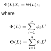
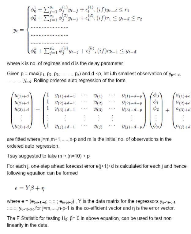
Stationarity is considered to be a desirable property under forecasting framework which ensures that the series is going to exhibit similar properties as observed in the past. More so, majority of the forecasting models assume stationarity of underlying series for prediction purpose. In this context, the series are checked for stationarity property using unit root tests (ADF and Zivot Andrews Test). Augmented Dickey Fuller Test (ADF) tests the hypothesis of presence of unit root in the DGP. ADF is an enhanced version of Dickey – Fuller Test (DF) which incorporates the lags of the variable in the model itself and checks for the presence of unit root. While ADF test incorporates the lags of variable in the model, it ignores the presence of structural breaks in the economy. Zivot and Andrews (1992) proposed to determine structural breaks endogenously which uses sequential test on full sample and defines dummy for each possible break point. The break date is chosen such that the t-statistic value of ADF test is minimum. Zivot and Andrews Test is different from Perron (1989) test which determines the structural break exogenously. The Zivot-Andrews Test identifies single break point (if it exists) which needs to be validated based on the prevalent economic condition. If the stationarity assumption is ensured, the series is expected to have same mean, variance and auto-correlation structure in future. Thus, characteristics of any stationary data generating process (DGP) can be analysed using measures of central tendency, variability and inter-dependencies. The time dependence of DGP involves auto-correlation among observations which need to be detected using ACF-PACF test. The central tendency and variability of any series, measured in terms of mean and variance, indicate the underlying feature of DGP and hence can be used as preliminary analysis of nature of the series. On the other hand, any DGP can exhibit majorly two types of properties – mean reverting and long term dependency (or long memory). The Hurst Exponent (Hurst, 1951) uses autocorrelation and its decay with lags to provide a score mechanism for judging the long memory property of any series. Hurst exponent value lies between 0 and 1 with higher Hurst value indicating long memory. Any Hurst value in the range of 0.5 to 1 means that a higher observation is followed by another high observation in adjacent pairs i.e. a high value followed by high values and low values followed by low values. Hurst exponent value of 0.5 relate those series having positive or negative auto correlation in short lags but the absolute value decaying at exponential rate. Any Hurst value between 0 and 0.5 would indicate a mean reverting property which means that any large values would be followed by small values and vice versa. Apart from these, we have used statistical test for testing suitability of threshold type non-linearity in the DGP. In this respect, another pre-check using Tsay’s F-Test has been used. The null hypothesis of Tsay’s test is as follows H0: Xt ~ AR(k) vs H1: Xt ~ SETAR Tsay’s test uses arranged auto regression and recursive least square for estimating the test statistic which follows F-distribution under H0 (Details of Tsay’s Test are furnished in Appendix I) 3.2 Models considered The models considered in this paper consists of linear and non-linear models. Linear models Auto Regressive Moving Average (ARMA) and Holt – Winters Exponential Smoothing techniques have been considered as part of linear models. ARMA model combines the auto regressive part and moving average models. Any ARMA model can be written as
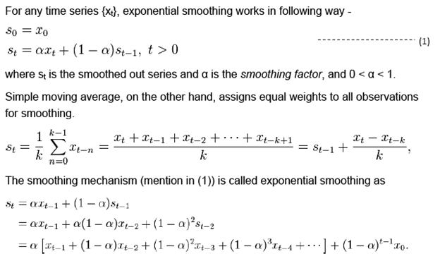
Exponential smoothing is technique used in time series to smoothen a series or to forecast. Contrast to simple moving average, exponential smoothing technique uses exponentially decaying weightage on older observations. It, in a way, accommodates higher weightage on the recent observations and lesser weightage on older observations. Detail of the exponential smoothing technique is provided in Appendix I. Non-linear models The non-linear models considered in this paper, can be classified into threshold models, cubic spline and artificial neural network model. The threshold models are further categorised into following
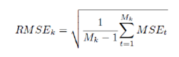
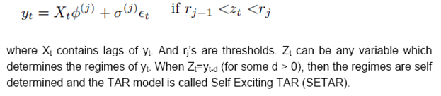
Self-exciting threshold autoregressive model is an extension of autoregressive model in a regime switching environment. The model consists of n-number (n being number of regimes) AR models and the switching among regimes is dictated by own lagged values of the variable which derives the name “Self Exciting”. In this paper, we have considered 2 and 3 regime SETAR only. On the other hand, STAR models are flexible from SETAR model in terms of smooth transition mechanism. Thus, observation at any point of time is the weighted average of AR models in each regime. Logistic STAR (LSTAR) model has been considered in this paper. The threshold values of non-linear threshold models are estimated endogenously by minimizing pooled AIC criteria. For more than 2 regimes, the second regime is estimated conditional on the first regime. The model parameters are estimated using the observations and the residuals are checked for robustness of the model. In this paper, we have used BDS Test and ARCH Test for checking heteroscedasticity in the residuals. Also ACF-PACF Test has been used for checking dependencies among residual terms. Apart from these, additive non-linear autoregressive model (AAR) derives from generalized additive class of models (proposed by Hastie and Tibshirani, 1990) which are represented as cubic regression splines. Artificial Neural Network (ANN) comprises computation models which are extensively used in machine learning and pattern recognition. Recently ANN has also been introduced in the time series modelling. Even though ANN can be generalized using multi-layer perceptron, the same comes with the cost of increasing parameter space. In this exercise, single perceptron ANN has been used for forecasting purpose. Details of the non-linear models have been furnished in Appendix I. Forecast Combination Combination of different forecasts can be made using different techniques like simple average, weighted average, median etc. However, the linear combination of forecast may no longer be optimal if the forecast error is non-Gaussian. Median forecast can be used as pooled forecast in such cases. Another advantage of using median forecast is that linear combination technique (eg. average) assigns equal weightage to forecast and thus, can be distorted due to presence of out-of-the-place forecast due to model error. In this paper, we have used median forecast as a measure of pooled forecast. 3.3 Performance comparison The data series have been segregated into training and test data set. While training data set has been used to determine the parameter of the model, the test data has been used for performing rolling forecast. The training and test data sets are so segregated such that test data does not involve any outlier. In case the test data is affected by any extreme values, the performance of rolling forecast would be affected to a significant extent. Also the test data set should not be so small that rolling forecast is affected by insufficient data points. Rolling forecast has been performed by incrementing the training data set every time and forecasting the next 4-quarter or 12-months horizon using the estimated models. The forecasts are compared against actual observations and RMSE is calculated using the following formula –
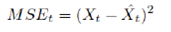
where MSEt is the mean square error at time point t and Mk is no. of rolling window of kth horizon forecast. MSEt is defined as
Models exhibiting lower RMSE value indicate better forecast capability. 4. Variables and Data Coverage The data used in this paper are macroeconomic indicators of India. These macroeconomic indicators can be classified into following general categories -
The training dataset for monthly data series has been restricted up to Mar-2011. Similarly, the quarterly data of GDP has been restricted up to Q4: 2010-11 for training. Following is the summary of observations of IIP and GDP data and their components
Majority of components of IIP are having mean reverting property (Hurst exponent <0.5), also these series suffer from very high coefficients of variation (CV> 1). Thus, forecasting of these series (having low Hurst exponent value and high volatility) would be difficult. The series which are having high Hurst exponent value and lesser variability are considered to be much more stable and hence can be easily tractable in nature. On the other hand, GDP being reported at quarterly frequency, the sectoral components of GDP exhibit similar nature but the variability of observations is comparatively much lesser than IIP. Only GDP-Agriculture and GDP-Mining are having relatively higher variability compared to others. In the subsequent section, we would try to associate the forecast performance using this basic attributes of the data. In this paper, the model parameters are estimated using full data set2. The lag order of ARMA models has been decided using minimizing AIC criteria while the order and delay parameters of non-linear models have been estimated by minimizing pooled AIC. The order of ARMA models and threshold values used in SETAR with 3 regimes and 2 regimes are furnished below –
Majority of IIP series are having low Hurst exponent values and high CV values which attributes to high volatility and mean reverting nature; are having higher RMSE indicating lack of fit. The data generating process of IIP having lower volatility (CV <1) and long memory property (Hurst >0.5) are better estimated through time series models compared to others. On the other hand, the series which have long memory property but are highly volatile in nature tend to have higher RMSE.
Compared to IIP series, majority of GDP series are found to be having lesser volatility and long memory property indicating better predictability. The rolling RMSE figures are lesser in magnitude than IIP series. Also, similar phenomenon has been observed in the RMSE values with respect to Hurst values and volatility.
The forecasting performance of naive models (linear and non-linear) when compared with respect to RMSE of rolling forecast mechanism, indicates no clear improvement of using non-linear models compared to linear models. For IIP series, the median forecast has been found to be performing better than linear and non-linear models in most of the series in short (1-6 months ahead) as well as long forecasting horizon (7-12 months ahead).
For GDP series, the data generating process is comparatively less volatile and has long memory property. The median forecast has been found to be out-performing than linear and non-linear models in 1-2 quarter ahead forecast horizon while the non-linear models are found to be performing marginally better than median forecast in 3-4 quarter ahead forecast for some series while median forecast is performing better for almost all series. The linear models are found to be having higher RMSE than non-linear and median forecasts, indicating lack of fit. For IIP series, in the short horizon (1-6 months), forecast combination (median) of linear and non-linear models are found to be marginally better performing than linear and non-linear models for IIP series. However, in the long horizon (7-12 months), non-linear models perform relatively better than the linear models as well as combination forecast (Table 8).
In case of GDP series, both short as well as long horizon combination forecast (median) has been found to be performing relatively better than linear and non-linear models. In this paper, we have compared the forecast performance of the linear model and non-linear naive models along with the performance of forecast combination for IIP and GDP data. Majority of IIP sub-component (sectoral and use-based classifications) series are having low Hurst exponent values and high CV values which attributes to mean reverting and high volatility nature; and are having higher RMSE indicating that even non-linear models fail to increase forecast accuracy for these series. The data generating process of IIP having lower volatility (CV <1) and long memory property (Hurst >0.5) are better estimated through forecast combination compared to naive models. The non-linear models, further, improves the forecast accuracy for these series. On the other hand, GDP series are having low coefficient of variation and relatively high Hurst value which indicates that the data generating process of GDP and its sub-components is relatively lesser volatile and has long memory property. Median forecasts are found to be out-performing naive models for forecasting quarterly GDP. For IIP series, in the short horizon (1-6 months), forecast combination (median) are found to be marginally better performing than that of linear as well as non-linear modelling framework. However, in the long horizon (7-12 months), non-linear models perform relatively better than the linear models as well as combination forecast. Whereas, for GDP series, forecast combination using median forecast, has been found to be performing relatively better for both short horizon as well as long horizon. Though non-linear models and combination forecast are found to be performing better than linear models for some variables, the same cannot be generalized across all series for all forecast horizons. Particularly, even if there is improvement of fit, the out-of-sample forecast error is significantly high which raises the question of overall forecast accuracy. Under this yard stick, the combination forecast (median) has been found to be consistently performing better than other model forecasts in most instances. This paper observes an improvement in forecast performance by combining forecasts obtained from different models (linear and non-linear) using median. Thus, combination of forecasts may be used instead of standalone forecast obtained either from linear or non-linear models for better tracking the macroeconomic series. @ The paper is authored by Anirban Sanyal (Email), Research Officer and Indrajit Roy (Email), Director of the Department of Statistics and Information Management, Reserve Bank of India, Mumbai. 1 Authors are thankful to Dr. Pulak Ghosh, Indian Institute of Management at Bangalore for his valuable comments. Views expressed in the paper are those of the authors and not of the organization to which they belong. 2 Using full data set indicates that entire time series observations were used for model identification. Bibliography Alina Barnett, Haroon Mumtaz and Konstantinos Theodoridis. "Forecasting UK GDP growth, inflation and interest rates under structural change: a comparison of models with time-varying parameters." Bank of England Working Paper 450, May 2012. Deschamps, Philippe J. "Comparing Smooth Transition and Markov Switching Autoregressive Models of US Employment." NBER Working Paper 6607, 2001. Gabriel Rodriguez, Michael J Sloboda. "Modelling nonlinearities and asymmetries in quarterly revenues of the US telecommunications industry." 2002. Gershen, Weigand A S and N A. "Time Series Prediction: Forecasting the Future and Understanding the Past." Addison - Wesley for Santa Fe Institute, 1994. Gweke, Meese R and J. "A Comparison of Autoregressive Univariate Procedures for Macroeconomic Time Series." Journal of Business and Economic Statistics, 1984. Liu, YueWu and Xiaonan. "Identifying and modeling with structural breaks: an application to U.S. Imports of Conventional Motor Gasoline data." NBER Working Paper 6607, 2008. Makridakis S, A Anderson, R Carbonne, R Fildes, M Hibon, R Lewandowski, J Newton, E Parzen, R Winkler. "The Accuracy of Extrapolation (Time Series) Methods: Results of a Forecasting Competition." Journal of Forecasting, 1982. Mitra, Ashok K. Nag and Amit. "Forecasting Daily Foreign Exchange Rates Using Genetically Optimized Neural Networks." Journal of Forecasting, 2002. Watson, James H Stock and Mark W. "A Comparison of Linear and Non-Linear Univariate Models For Forecasting Macroeconomic Time Series." NBER Working Paper 6607, 1998. White, Swason N R and H. "A Model Selection Approach to Assessing the Information in the Term Structure using Linear Models and Artificial Neural Network." Journal of Business and Economic Statistics, 1995. Appendix Appendix I: Details of Linear and Non-linear Models used A. ARIMA: ARIMA (p,d,q) is defined as
Where Zt are white noise B. Exponential Smoothing Exponential smoothing is a technique to produce smoothed out data from a noisy time series data or making forecasting using smoothing techniques. Exponential smoothing is considered to be an efficient technique for removing fluctuations caused by random noise. Exponential smoothing assigns decreasing weight to past observations in order to smooth out the extra noises in the data.
Different Exponential Smoothing Techniques There are various types of exponential smoothing that are quite frequently used in time series analysis –
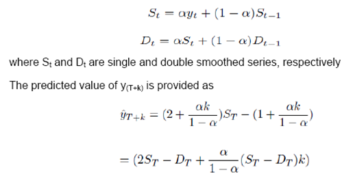
Simple exponential smoothing (mentioned in (1)) is quite simple in nature and cannot be adopted in case the underlying data contains trend and/or seasonal factors. Hence, double and triple exponential smoothing techniques are used to take care of the trend and seasonal component, respectively. Double Exponential smoothing Double exponential smoothing considers smoothing of the raw data as well as the estimated trend component separately and uses those estimates to predict the future values. Majorly two methods are used under double exponential smoothing – Holt-Winters double exponential smoothing Holt-Winters double exponential smoothing uses smoothing in 2 stages –
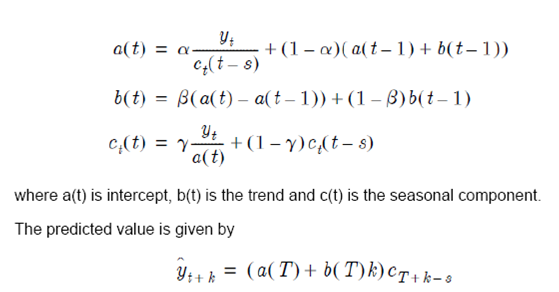
Triple Exponential Smoothing Triple exponential smoothing considers the seasonal factors also in the smoothing mechanism. The method estimates the trend and seasonal components using the weighted values of trend line falling in cycle of length L. The smoothed series is generated using following iteration
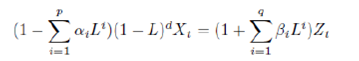
C. Threshold Auto Regressive Model TAR Models were first proposed by Tong in 1982 and were discussed in detail by Tong (1990). The TAR Models are simple in nature and are able to capture high degrees of non-linearity in the data. A general form of TAR model is given by
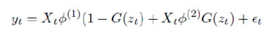
Smooth Transition Auto Regressive Model While SETAR incorporates the regime switching process of data generating process (DGP), the smooth transition among regimes is not captured in the model. Thus Smooth Transition Auto Regressive Model (STAR) was proposed, which incorporates the switching behaviour using continuous transition mechanism. A generalized form of STAR model is represented as follows –
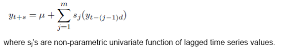
where G() is some distribution function governing the switching mechanism. Typically in STAR model, G is taken to be logistic and exponential distribution, respectively called as LSTAR and ESTAR Model. Since our focus of study is confined to Y-o-Y growth rates which can have negative values also, we stick to LSTAR model only. D. Additive Non-linear Autoregressive Model (AAR) Hastie and Tibshirani (1990) advocated the use of Generalized Additive Models (GAM). However, the order of GAM poses a problem. Hence, Wood and Augustin (2002) proposed to use cubic regression spline and thus, introduced the concept of Additive Non-linear Autoregressive Model (AAR).The functional form of AAR model is represented as below –
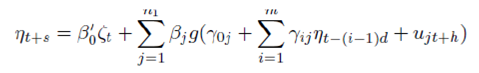
E. Artificial Neural Network Model (ANN) Artificial Neural network is considered to be the most generalized form of any model. However, any multi layer neural network involves many parameters, which require to be estimated using the data. For the sake of simplicity of the model, here we have considered single layer neural network framework which can be represented as follows –
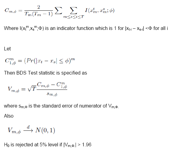
where g() is logistic function. F. BDS Test Brock, Dechert and Scheinkman introduced BDS Test in 1987. The test performs testing of null hypothesis of independent and identical distribution (iid) for the purpose of identifying non-random chaotic dynamics. However, Brock, Hsieh and LeBaron (1991) and Barnett, Gallant, Hinich, Jungeilges, Kaplan and Jensen (1997) showed that BDS possess higher power against linear and non-linear alternatives. Here BDS is used to identify the hidden non-linearities that are present in the data after fitting a linear model. In case the null hypothesis cannot be rejected, then the original linear model cannot be rejected. The test statistic for BDS Test is given by
G. Tsay’s F-Test Tsay’s Test procedure provides a robust test procedure for testing the presence of threshold non-linearity in any data generating process. The null hypothesis and alternative hypothesis of Tsay’s Test states the following – H0: Xt follows linear process vs H1: X1 have SETAR(j) process One of the major challenge in testing the hypothesis is that the thresholds are observable under H1 only. Tsay (1989) proposed F-test using auxiliary regression in order to avoid dealing with the threshold directly. The basis of Tsay’s test lies on arranged auto regression and recursive least square technique. A k-regime SETAR Model is given by
Appendix II: RMSE of Rolling Forecast (For IIP and GDP Series)
| |||||||||||||||||||||||||||||||||||||||||||||||||||||||||||||||||||||||||||||||||||||||||||||||||||||||||||||||||||||||||||||||||||||||||||||||||||||||||||||||||||||||||||||||||||||||||||||||||||||||||||||||||||||||||||||||||||||||||||||||||||||||||||||||||||||||||||||||||||||||||||||||||||||||||||||||||||||||||||||||||||||||||||||||||||||||||||||||||||||||||||||||||||||||||||||||||||||||||||||||||||||||||||||||||||||||||||||||||||||||||||||||||||||||||||||||||||||||||||||||||||||||||||||||||||||||||||||||||||||||||||||||||||||||||||||||||||||||||||||||||||||||||||||||||||||||||||||||||||||||||||||||||||||||||||||||||||||||||||||||||||||||||||||||||||||||||||||||||||||||||||||||||||||||||||||||||||||||||||||||||||||||||||||||||||||||||||||||||||||||||||||||||||||||||||||||||||||||||||||||||||||||||||||||||||||||||||||||||||||||||||||||||||||||||||||||||||||||||||||||||||||||||||||||||||||||||||||||||||||||||||||||||||||||||||||||||||||||||||||||||||||||||||||||||||||||||||||||||||||||

شارك هذه الصفحة:


بھارت موبائل ایپلی کیشن کے ریزرو بینک کو انسٹال کریں اور تازہ ترین خبروں تک فوری رسائی حاصل کریں!
ہماری ایپ انسٹال کرنے کے لیے QR کوڈ اسکین کریں۔


صفحے پر آخری اپ ڈیٹ:


