 IST,
IST,
Report of the Internal Technical Group on Seasonal Movements in Inflation
Executive Summary 1. Communication of inflation rate appropriately is important, as economic agents and financial markets are expected to form their price expectations based on official published figures. Publication of inflation figures, not consistent with actual movements in price series, i.e., WPI/CPI, may result in formation of biased expectations. 2. In general, inflation rate is presented as variation in price indices with respect to a previous period, such as, annual point-to-point, month-over-month, etc. In the Indian context, official inflation rate is measured based on annual point-to-point basis change in the Wholesale Price Index (WPI). Measurement of inflation rate based on annual changes in prices or annualisation of changes over shorter period (month/quarter) is necessary for relating inflation with financial indicators (e.g., interest rates). 3. Analysis of annual point-to-point inflation reveals that, these are susceptible to the base effect. An alternative method of measuring inflation could be month-over-month variation in WPI, using seasonally adjusted data. However, such inflation rate exhibits high volatility, and does not exhibit appropriate stable signals about price changes. Measuring inflation i.e., price variation over a fixed base (say, end-March data of the previous financial year), also provides useful information regarding price dynamics during the year. These measures of inflation, though appropriate for assessing inflation during the year, have limitations, as they do not provide (appropriate) annualised inflation rates. 4. Similarly, annual inflation rates worked out on the basis of moving average of price indices of previous 4/12/52 weeks exhibit lower variability due to increased smoothening and captures almost all the important turning points by reducing noise elements. However, it is biased towards past data and has a centre, which becomes increasingly remote as the length of observations considered increases. Such measures of inflation rate become less useful for measuring current (underlying) inflation. 5. Internationally, the most common method of inflation measurement is the annual point-to-point change in consumer price index, though annualised variations over shorter horizon are also used. For example, Bank of England, in its Inflation Report, presents inflation rate, based on the annual percentage change, for each month of the year. Similarly, European Central Bank presents the inflation rate, based on annual percentage change on monthly data. Bank of Japan presents annualised, as well as monthly inflation rates, for each month of the year. In many of the Central Banks, the month-over-month inflation rate is obtained, using seasonally adjusted data. 6. In the Indian context, X-12-ARIMA and its earlier variants, which are also used by the Bureau of Labour Statistics (BLS), USA, have been used since 1980, for obtaining seasonal adjustment in price data. A detailed analysis, as carried out by the Group, found that, seasonal factors of WPI and CPI series, obtained by using X-12-ARIMA procedure, reveal that prices firms during the period August – November. Incidentally, this period encompasses occurrence of monsoon, when there could be supply bottlenecks, and festival seasons when there could be demand escalation. These results appear to be consistent with expected price changes during the year, on account of seasonal factors. Thus, X-12-ARIMA appears to be appropriate for seasonal adjustment of WPI and CPI series during the year. 7. All the price series in India (viz., WPI, CPI) have peak/trough months around same time of the year mainly due to seasonality in food prices, which are the major source of seasonality in all price indices. Generally, price level (not inflation rate) is likely to show upward bias during August-November, whereas, for the remaining months, the price level should show the downward bias. Seasonality is more profound in various CPIs as compared to WPI. Although the impact of seasonality is much pronounced in prices of Fruits and Vegetables; relatively moderate seasonality in some foodgrains, viz., Wheat, Pulses, etc., also influence the seasonal behaviour of aggregate price index due to their high weights. Excluding these commodities, the degree of changes in WPI, due to seasonality, is relatively low. Seasonality in Manufactured Products is very low and emanates from price changes for Food Products. 8. Finally, the analysis revealed that, inflation rate based on annual point-to-point basis, supplemented with month-over-month and fixed base (using seasonally adjusted price series) provide better signal regarding price dynamics in the Indian economy. Report of the Internal Technical Group on Contents Chapter Topic Chapter-II Genesis and Presentation Issues on Inflation: Some Stylised Facts Chapter-III Methodology for Seasonality Adjustments Chapter-IV Measurement of Inflation - International Practices Chapter-V Seasonality in Price Measures: The Indian Case Chapter-VI Comparative Analysis of Different Inflation Measures Chapter-VII Conclusions and Recommendations Annexure Annexure-I Seasonal Adjustment: Description of the Methods Report of the Internal Technical Group on Introduction I.1 Genesis of the Group 1.1 In order to examine the pattern of seasonal behaviour of Inflation in India, and to further strengthen analytical inputs for the conduct of Monetary Policy, the Reserve Bank of India set up an Internal Technical Group on 'Seasonal Movements in Inflation', vide, Memorandum issued by Deputy Governor, Dr. Rakesh Mohan on September 11, 2007. 1.2 The constitution of the Internal Technical Group is as follows:
1.3 The Terms of Reference of the Internal Technical Group are as given below: (i) To suggest appropriate method to estimate seasonal factor to be used to gauge the inflationary pressure in Indian Economy during the year. 1.4 The memorandum authorized the Technical Advisory Group to co-opt any other person/s for specific deliberations. I.2 Scheme of the Report 1.5 The Group deliberated in detail on various issues regarding the seasonal behaviour of inflation during the year and also the different ways of measuring headline inflation. In this context, the Group examined, in detail, different ways of presentation of inflation, viz., annual point-to-point inflation based on weekly WPI, inflation based on moving average of 4/12/24/52 weeks of WPI, fixed base, month-over-month, etc. Further, this Group examined the nature of seasonality in WPI at aggregate and disaggregate level, identifying the commodities in WPI basket showing high seasonality. Similarly, the Group also examined the nature of seasonality in various CPIs. Based on these deliberations and the background empirical work undertaken, the Group finalised the Report. This Report is organised in seven chapters. Chapter II presents genesis and presentation issues of inflation. Chapter III gives various procedures for seasonal adjustment. Chapter IV discusses the international practices, for the presentation of inflation. Chapter V provides the seasonality in price measures, in India. Chapter VI gives comparative analysis of different inflation measures. Conclusions and recommendations are given in Chapter VII. I.3 Acknowledgements 1.6 The Group is extremely thankful to Shri Dipankar Biswas and Smt. Arti Sinha, Research Officers, Forecasting Division, Department of Statistical Analysis and Computer Services, and Shri. Binod B. Bhoi, Research Officer, Department of Economic Analysis and Policy, for their untiring contribution towards completion of this Report. Genesis and Presentation Issues on Inflation: Some Stylised Facts II.1 Genesis 2.1 In India, the official inflation rate is based on the annual point-to-point increase in the Wholesale Price Index (WPI), which is a weekly index, released with 13 days’ time lag. This practice is different from other major countries where inflation is based on Consumer Price Index (CPI), which is generally a monthly index. As such, the periodicity of release of official inflation in India is higher than in other major countries. Since commodity level indices are also released with the aggregate WPI, it is easier to study the major sources of price changes. In addition, there are four official series on CPI, viz., for Industrial Workers (IW), for Urban Non-Manual Employees (UNME), for Agricultural Labourers (AL), and for Rural Labourers (RL), which also cover some basic services, whereas, WPI is only commodity price index. Inflation rate can also be calculated from national accounts aggregates, viz., Gross Domestic Product (GDP) deflator, Private Final Consumption Expenditure (PFCE) deflator, and Gross Domestic Capital Formation (GDCF) deflator, which are available with a lag and also undergo revisions for a long time making it difficult for put to use for monetary policy decisions. 2.2 Reserve Bank’s Annual Policy Statement for Monetary Policy, which is released every year in April, provides indicative projections of annual inflation for policy purposes. This projection is reviewed every quarter as per current practice, and risks and challenges in bringing inflation towards the desired trajectory are spelled out clearly in the Policy Reviews. The inflation projection is generally understood as being measured by variations in wholesale price index (WPI) on an annual point-to-point basis. Furthermore, it is generally understood that inflation is represented by the year-on-year variation in the wholesale price index (WPI), although analysis based on consumer prices are also used for assessing inflationary pressures in the economy. The Reserve Bank also monitors price movements based on various CPIs, commodity-level indices and contextual measures (excluding commodities with volatile prices). 2.3 As measurement issues related to inflation and their presentations for policy purposes have implications for transparency and hence credibility of monetary policy, it is pertinent to be vigilant on certain aspects related to the presentations of the inflation rates. The most important aspect that has a direct bearing on the whole issue of measurement of inflation relates to the presence of "noise" in the form of seasonal factors, or any other (temporary) supply shocks affecting prices, which boils down to what engineers call a "signal extraction problem". This involves eliminating "noise" in inflation measures, and trying to maximize the amount of signal. By eliminating seasonal influences, policymakers can get a better sense of underlying trends in inflation rate. Perhaps, one of the appropriate characteristics of the measure of inflation rate should be that it should not show wide volatility, which is also sought to be achieved by using an aggregate price index rather than working with relative price of major commodities. Thus, the price volatility, in case of few commodities, or at a few places, is expected, but at the aggregate, such variabilities should smoothen out. 2.4 From the policy aspect, these issues are important since, economic agents including general public are expected to base their decisions on the officially released inflation data, which need to be credible. Thus any presentation of inflation data, which is perceived to be inconsistent with actual price changes in the economy, may generate (biased) market expectations further complicating policy-makers choice both in terms of analysis as well as policy response. 2.5 In the Indian context, annual point-to-point inflation often shows wide and abrupt variability, many a times, during the year. Therefore, there is a need to assess whether such changes in inflation rate are reflection of actual changes in price level (viz., WPI), or due to (temporary) seasonal factors, or merely due to some statistical phenomena, such as base effect, etc. In this background, this Report examines the various measures of inflation rate – their merits and demerits; nature of seasonality in WPI and CPIs. II.2 Measurement of Inflation 2.6 The general measure of inflation could be given as:
where, II.2.1 Measure of Inflation over the Year 2.7 The annual point-to-point inflation is defined as a percentage change in the price level at a point of time as compared to the price level a year ago. Although this inflation rate is widely used across the countries for monetary policy purposes and in financial markets, it has serious limitations, if there were abrupt price variations twelve months earlier, its effect would be reflected in the current inflation rate, though the current price level may be very stable, or even, it may be showing moderation. Table 1 shows the annual point-to-point inflation rate for the period April 2001 to March 2007, based on end-of-month WPI-All Commodities. Table 1: WPI-All Commodities (End-of-Month) and Annual Point-to-Point Inflation
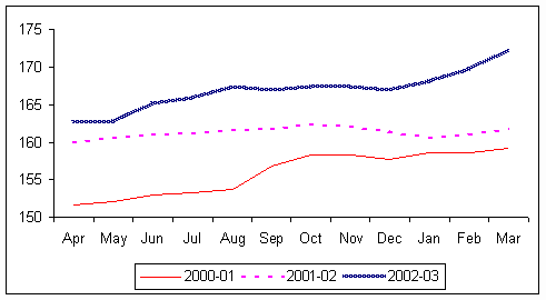
Chart 1: WPI-All Commodities
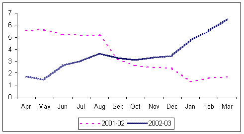
Chart 2: Annual Point-to-Point Inflation
2.8 During 2001-02, the movement of WPI-All Commodities was more stable, as compared to that during 2000-01 and 2002-03. As a result, the annual point-to-point inflation for 2001-02 and 2002-03, showed opposite movements. While the price index was stable during the year, there was wide variability in the annual point-to-point inflations due to its volatility in the previous year (base effect) (Chart 1 and Chart 2). A similar phenomenon was observed recently. From September 2006 to January 2007, the annual point-to-point inflation increased from 5.41 per cent to 6.69 per cent, and as a result, a public opinion was formed that, the inflation in India was becoming too high, and perhaps was moving beyond the control (of monetary authority). However, during the same period, WPI increased very moderately from 208.3 to 209.0. Thus, during the five-months period, inflation rate increased by 1.28 percentage point, though the price index increased by only 0.33 per cent which reflected fallacies of base effect (Table 2). Table 2: Movements of Weekly WPI and Annual Point-to-Point Inflation
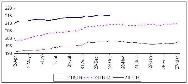
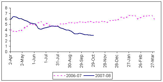
2.9 In fact, the current phase of a fall in inflation rate from July 2007 to October 2007 is also purely as a result of base effect. During this period, the inflation rate has declined from 4.70 per cent to 2.97 per cent, whereas, WPI for this period has increased from 213.9 to 215.1 (Chart 3 and Chart 4). It is useful to note that, the consumers are affected by the actual price level (i.e., WPI) and not inflation rate. Similarly, for converting many of the macro variables from their nominal to real values, price levels are used. For example, obtaining GDP components, real demand for money/credit/real effective exchange rate, etc., WPI is used. Chart 3: Movements of Weekly WPI
Chart 4: Annual Point-to-Point Inflation
2.10 While there can be several reasons for abrupt change in domestic inflation rate, the major sources of its volatility include sudden domestic supply shock (e.g., prices of agricultural commodities), international demand /supply conditions (e.g., global crude oil/steel/foodgrains prices) and base effect. While the first two sources affect the price level, the third affects only the inflation rate in which case the volatility introduced by it should not be alarming. In case, such incidents are not explained properly, there is a risk that, economic agents may form an opinion of (actual) price rise in the economy. 2.11 It is pertinent to note that, in case of developed economies, also similar problems persist. These results are reflected from Table 3 giving the seasonally unadjusted Consumer Price Index (US city average) for All Items, and the year-on-year inflation. Thus, while the problem of abruptness due to base effect persists even in developed countries, the problem is less severe as inflation rate average and dispersion in their case is low as for most commodities, converge in the range of 2.0 to 4.0 per cent. In India, the issue needs more attention as we have higher average and dispersion. Table 3: Movements of Monthly CPI and Year-on-Year Inflation
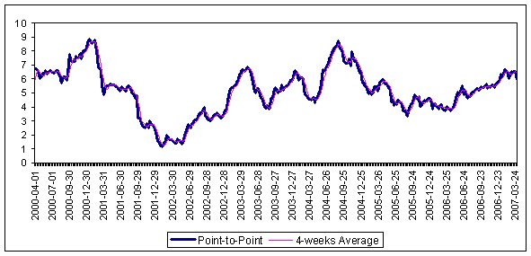
II.2.1.1 Measures of Average Inflation based on Weekly Price Indices 2.12 In the case of annual point-to-point inflation based on weekly data, the main limitation is that, as a result of base effect, it shows wide variability. This limitation could be rectified by taking the moving averages of indices, with varying frequencies. The concept of varying frequency is incorporated, in order to construct the indices in monthly, quarterly, and annual mode. The frequencies are 4-weeks, 12-weeks, and 52-weeks, respectively. II.2.1.1.1 4-weeks Moving Average Inflation 2.13 In order to capture the movements of WPI, as well as the inflation, on a monthly basis, the 4-weeks moving average is used. In this method, the average of WPI for the 4-weeks (including the current week) is compared with the similar price index (average of 4 weeks) of the corresponding period of the previous year, and annual point-to-point inflation is worked out. The movement of annual inflation, based on 4-weeks moving average, though similar to that of annual point-to-point inflation, shows less variability (Chart 5). Chart 5: Movements of Annual Inflation
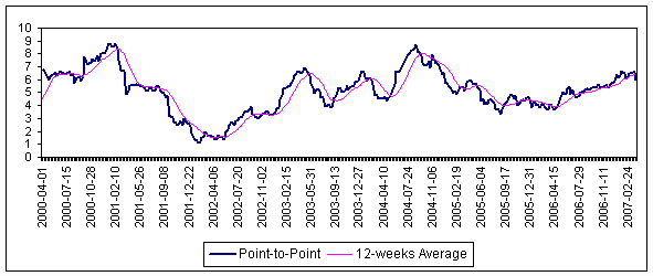
II.2.1.1.2 12-weeks Moving Average Inflation 2.14 In this method, the average of WPI for 12-weeks (including the current week) is compared with the similar number of the previous year, and annual point-to-point inflation is worked out. The movement of annual inflation, based on 12-weeks moving average, is more smooth, as compared to the annual point-to-point inflation (Chart 6). However, it captures the cyclical movement of annual point-to-point inflation with 1 to 2 months lag period. Chart 6: Movements of Annual Inflation
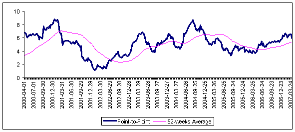
II.2.1.1.3 52-weeks Moving Average Inflation 2.15 Similar to the 12-weeks moving average of WPI, in this method, the average of WPI for the 52-weeks (including the current week) is compared with the corresponding average of WPI of 52 weeks of the previous year, and the annual point-to-point inflation is obtained. The annual inflation, based on 52-weeks moving average captures the cyclical movement of annual point-to-point inflation with lag of more period (Chart 8). Chart 8: Movements of Annual Inflation
2.16 Chart 9 indicates that, the variability1 of the annual inflation rate decreases as the frequency of moving average of weekly indices increases. It reveals that, the increase in the number of weeks, for averaging the price series, eliminates noise from the series. While 52-weeks moving average eliminates more noise, it is centred around a period, which is six months ago and would not be reflecting the "current" inflation rate. Among all the weekly averages, taken into consideration, the annual inflation, based on 12-weeks average captures the inflationary pressure, well in time and captures turning points with a minimal lag (of 1 or 2 months). Chart 9: Standard Deviation of Annual Point-to-Point Inflation
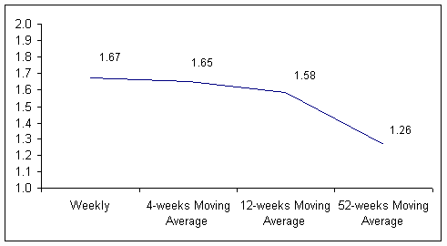
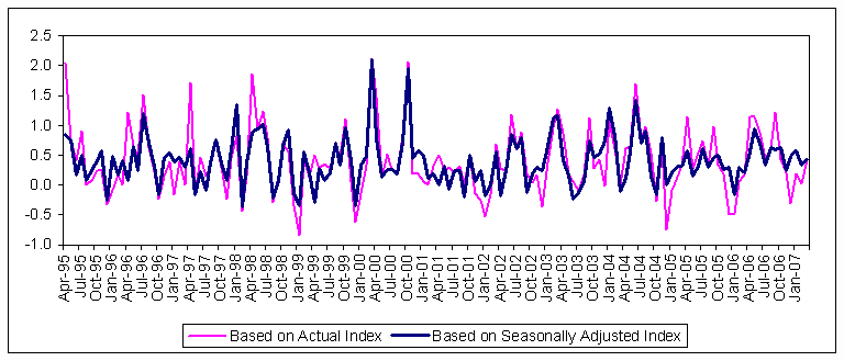
II.2.1.2 Remarks 2.17 The annual point-to-point inflation represents price movements, with respect to the previous year, and does not fully reveal price changes during the current period. So, it is necessary to look at the price variations during the year to which a few next paras are devoted. II.2.2 Measure of Inflation during the year 2.18 Measures of inflation, as documented in Section II.2.1, represent price rise over the period, and has the limitations that, they do not reveal price rise, during the year. In order to overcome these limitations, there have been suggestions, to work out inflation based on month-over-month WPI (or, CPI, etc.)2. Since WPI is prone to be affected by seasonal factors, the month-over-month variations are worked out, after deseasonalising the price indices. Similarly, price changes have been worked out, based on quarterly data. For deseasonalisation, X-12 ARIMA methodology can be used. A brief of this methodology is presented in the next chapter. II.2.2.1 Monthly Measure of Inflation 2.19 The monthly inflation is measured by formula (1), by taking Pt-1, instead of Pt-12, i.e., price indices, of the consecutive months, are considered to measure this inflation. The price index is prone to have seasonal fluctuations. In order to remove seasonality, the price indices are seasonally adjusted. Moreover, the monthly inflation, based on the seasonally adjusted index, is less fluctuating as compared to that based on the unadjusted price index (Chart 10). A comparable estimate of annualised inflation can be obtained by multiplying the monthly inflation by 12 (Table 4). Chart 10: Monthly Inflation – Based on WPI-All Commodities
Table 4: Measure of Inflation based on Seasonally Adjusted Monthly WPI-All Commodities
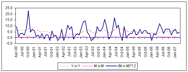
2.20 At first, the seasonally adjusted monthly series of the WPI-All Commodities is considered, and the monthly inflation (M-o-M) is measured. Considering the seasonally adjusted monthly inflation, and multiplying it by 12, an estimate of the annualised inflation for the corresponding month is obtained. 2.21 Chart 11 shows the movements of monthly inflation (M-o-M), and year-on-year inflations (Y-o-Y), for the period April-2000 to March-2007. The estimate of annualised inflation (i.e., (M-o-M)*12) has more variability, as compared to the year-on-year inflation. The main limitation of this procedure is that, the annualised measure of inflation is highly volatile, as price revisions with high frequency introduce greater volatility in measures based on recent base compared to those based on distant base, as well as for the reasons given in para 2.12. Also seasonal adjustment for monthly data based on standard methods has limitations, in Indian context, as festivals do not follow Gregorian calendar (e.g., Holi can fall in March/April, whereas Diwali can come in October/November) and such shifts in seasonality create further issues in inflation measurement based on both seasonally adjusted as well as unadjusted data. Further, in case annualised inflation rate is obtained from month-over-month inflation rate, by multiplying the same with 12, the noise gets amplified. Chart 11: Movements of Year-on-Year and Monthly inflations
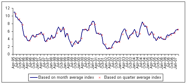
II.2.2.2 Quarterly Measure of Inflation 2.22 In the case of measuring monthly inflation, the WPI-All Commodities, for the consecutive months, were used. Besides this, one may think of the quarterly inflation measure, as it’s major advantage is that, it has correspondence with national income aggregates. For measuring quarterly inflation, the price indices are averaged on quarterly basis. The frequency of the price index series is weekly. For generating quarterly index series, the average of the weekly indices, included in the quarter, or the index corresponding to the last week of the quarter, is considered. Moreover, the quarterly inflation should be measured by using the seasonally adjusted quarterly price indices. Among all these three measures, the quarterly inflation, based on the seasonally adjusted price series, has lowest variability (Chart 12). Chart 12: Movements of Quarterly Inflation based on Actual and Seasonally 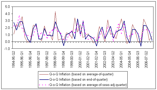
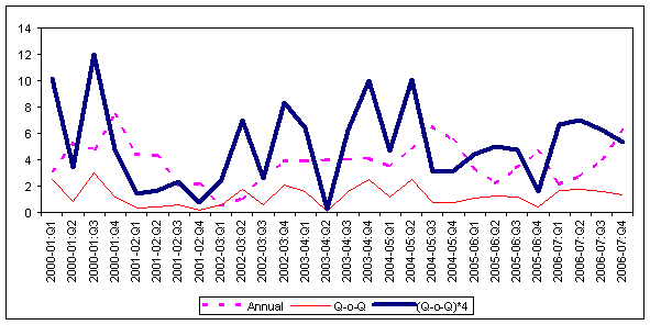
2.23 A comparable estimate of the annual inflation, for a quarter, is measured by using the quarterly inflation (i.e., Q-o-Q), during a financial year. The quarterly inflation is multiplied by 4, to obtain the annualised estimate of inflation for that quarter. The movement of such estimate is compared with the year-on-year inflation (Y-o-Y). Table 5 and Chart 13 show the movements of these estimates of inflation. The year-on-year inflation has less variability, as compared to the annualised estimate of inflation. The limitations of this procedure continue to be similar as for the month-over-month inflation. Table 5: Measure of Inflation based on Seasonally Adjusted
Chart 13: Movements of Annual and Quarterly inflations
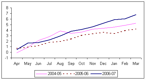
II.2.2.3 Fixed Base Inflation 2.24 In order to remove the vitiations created by strong base effects and focus more on intra-year variations, inflation is often measured by fixing the base to some time point. Generally, the last week/month of the previous financial, or calendar year is taken as the base, for measuring the inflation of the current year. In the Indian context, the end-week or, the average of weekly price indices of March price index could be taken as the base, for measuring inflation during the course of the financial year. 2.25 Chart 14 shows the fixed base inflation during the period April 2004 to March 2007, based on seasonally adjusted WPI-All commodities series. It may be noted that, the high inflationary pressure was observed during December-March 2006-07, as compared to the same period of 2004-05 and 2005-06. Chart 14: Fixed Base – Monthly Inflation
2.26 Table 6 indicates the merits and demerits of different measures of inflation. Table 6: Measures of Inflation – Merits and Demerits
II.2.3 Remarks 2.27 The inflation, measured during the year, is prone to be affected by seasonal fluctuations. In order to measure the extent of seasonality, formal statistical procedures have been developed. Some of these are discussed in Chapter III. X-12 ARIMA, developed by US Census Bureau, is the widely used procedure for seasonal adjustment of a series. Methodology for Seasonality Adjustments III.1 Introduction 3.1 Price data are used for different purposes by different groups. Accordingly, whether the data should be adjusted or not depends on the specific purpose of the use. Seasonally adjusted data are usually preferred in the formulation of economic policy and for economic research, because they eliminate the effects of changes that normally occur at the same time and in about the same magnitude every year, due to variety of seasonal factors. Seasonal price increases may not reflect the inflation persistence thereby necessitating special treatment in the formulation of policy. On the other hand, the unadjusted price data captures the actual prices paid by consumers in their consumption of the basket of goods and services and hence better reflects the cost of living. Therefore, unadjusted data are of interest to consumers and are used extensively for escalation purposes, wage bargaining contracts and pension plans, etc. 3.2 Typically, many seasonally observed macroeconomic time series are characterised by a trend, seasonal, nonlinear and a few outlier components. The outliers often result from changes in measurement systems or exogenous events like strikes. Nonlinearity often appears as regime-switching behaviour, in the sense that recessions may require a different model than expansions. Hence, nonlinearity tends to get associated with the business cycle. Thus, as the interest in analysing macroeconomic data generally concerns identifying the trend and the business cycle, it is necessary to somehow take care of that seasonality. This may help in generating out-of-sample forecasts for the next period, in searching for common patterns and thereby reduce the need for more model parameters, and may facilitate the analysis of dynamics and causal relationships. Furthermore, seasonal movements may be regular, yet they may be subject to changes in pattern over time. These changes are most commonly thought to evolve in a stochastic rather than a deterministic way. Seasonality is generally taken care of by incorporating some description of seasonality in an econometric model or by applying statistical techniques to get rid of the intra-year fluctuations, one way or another. 3.3 The idea behind seasonal adjustment, thus, is to remove the effects of recurring seasonal influences from macroeconomic data series, including consumer prices. The adjustment process quantifies seasonal patterns and then factors them out of the series to permit analysis of non-seasonal price movements for better macroeconomic analysis and policy. The US Bureau of Labour Statistics derives the seasonal movement of the overall (all-items) index and other aggregations by aggregating seasonally adjusted component (sub-group) indices. 3.4 Although seasonality may be easy to understand in theory, it is extremely difficult to remove. Seasonal adjustment does very little to reduce short-run, monthly variation in inflation data. Bryan and Cecchetti (1995) express the view that it would be advantageous to seasonally adjust inflation data at the aggregate level. 3.5 One of the simplest procedures for eliminating seasonal impact on any of the macro series, is to work out its year-on-year growth rate. For example, when we work out annual point-to-point inflation, it automatically eliminates seasonal impact on WPI. However, in order to assess the inflationary pressure during the year, it may be useful to deseasonalise WPI and work out the desired variation. 3.6 As regards, different procedures of eliminating seasonality, for more than hundred years, statisticians and economists have dealt with the simple procedure of decomposition of time series into trend, cycle, seasonal and irregular component. One important part of this analysis was the estimation and removal of the seasonal component to get a clearer picture of the state of the economy. They are usually defined in the following way: a) Trend is a slow variation over a long period of years, generally associated with the structural causes of the phenomenon in question. In some cases, the trend shows a steady growth, in others, it may move downward as well as upward. b) Cycle is a quasi-periodic oscillation characterised by alternating periods of expansion and contraction in most cases it is related to fluctuations in economic activity. c) Seasonal variations represent the effect of climatic and institutional events that repeat more or less regularly each year. d) Irregular fluctuations represent unforeseeable movements related to events of all kinds. These fluctuations are supposed to have a stable random appearance but, in some cases, extreme values may be present. These extreme values, or outliers, have identifiable causes, such as strikes or floods, and, therefore, can be distinguished from the much smaller irregular variations. III.2 Statistical Techniques for Seasonal Adjustment 3.7 In the recent period, as a result of the development in computer science and in stochastic theory, several new methodologies have been developed for seasonal adjustment of time series. The various procedures are DAINTIES, Seasonal Adjustment at Bell Laboratories (SABL), 'Berlin method' BV4, TRAMO/SEATS, X-11/ X-12-ARIMA. Among them, the most prominent are TRAMO/SEATS, X-11/ X-12-ARIMA. These two procedures are discussed below. III.2.1 TRAMO/SEATS 3.8 'Time Series Regression with ARIMA Noise, Missing Observations and Outliers' (TRAMO) is a program for estimation and forecasting of regression models with possibly non-stationary ARIMA errors and any sequence of missing values. The program interpolates these values, identifies and corrects for several types of outliers, and estimates special effects such as Trading Day and Easter and, in general, intervention variable type effects. SEATS ("Signal Extraction in ARIMA Time Series"), is a program for estimation of unobserved components in time series. The trend-cycle, seasonal, irregular and perhaps transitory components are estimated and forecasted with signal extraction techniques applied to ARIMA models. The two programs are structured so as to be used together both for in-depth analysis of a few series or for automatic routine applications to a large number of series. When used for seasonal adjustment, TRAMO pre-adjusts the series to be adjusted by SEATS. TRAMO/SEATS is developed by Maravall and Gomez and originated by a program from Burman (1980). Further details of this procedure are given in Annex I at the end. III.2.2 X-11/X-12-ARIMA 3.9 Among all these, X-11/X-12 ARIMA have emerged the widely used procedure across the world, and the Reserve Bank of India (RBI) has been using the same for obtaining seasonal factors for macro-variables relating to the Indian economy. An article relating to this aspect is being published in the RBI Bulletin regularly. The most widely used method for seasonal adjustment is the CENSUS X-11 method from the Bureau of the Census in the USA and its variants. The first computer based method was developed in 1954 and was known as CENSUS I method. This method was upgraded to the method X-11 in 1965 by Shiskin. X-12 ARIMA is an enhanced version of the X-11 Variant of the Census Method II seasonal adjustment programme. The procedure makes multiplicative/additive adjustments of a time series and creates an output data set containing the adjusted time series and intermediate calculations. Further details of this procedure are given in Annex I at the end. Measurement of Inflation - International Practices IV.1 Measurement 4.1 As regards the international practices for measuring inflation, the general practice is to provide year-on-year variation in the indices as observed in the reports of Bank of England, Bank of Japan, Sveriges Riksbank, IMF, OECD, etc. According to the monthly report of the Deutsche Bundesbank, the inflation measured on the Harmonised Index of Consumer Prices, for the euro areas, are reported as the annual percentage change for each month of the year. There are, however, instances where month over month inflation rate (without annualising) have also been presented. For, example in case of U.S. Bureau of Labor Statistics (BLS) and National Statistics, U.K, the rise in CPI month over month, both for seasonally adjusted and unadjusted data, are presented. IV.1.1 OECD 4.2 The analysis of price changes is central to the analysis of macroeconomic conditions. Generally, consumer price indices (CPI) are seen as one of the key indicators of price changes and are often used as the measure of inflation in each of the countries under OECD. In general, only one official measure of the CPI exists per country. In recent years, countries have started to place more emphasis on presenting a variety of price measures that are available and explaining how they can be used for different purposes. The Main Economic Indicators (MEI) publication contains a range of indicators of price change for the OECD member countries and for the OECD country groupings or zones. IV.1.2 U.S. Bureau of Labor Statistics (BLS) 4.3 As per BLS, the media generally reports various aspects of the inflation such as:
IV.1.3 Bank of England 4.4 As per the current practice, the Bank of England uses annual per cent change in CPI, for each month of the year. The inflation target is measured by the 12-months average on the CPI. During 2001, the Monetary Policy Committee presented a new measure of core inflation for the United Kingdom. This is based on the same goods and services used in the measurement of RPIX inflation, weighted by the persistence of their past inflation rates to derive a persistence-based measure of retail price inflation, or RPIXP for short. This differs from RPIX, which weights individual price components by their importance in households' budgets. IV.1.4 Sveriges Riksbank 4.5 For each month of the calendar year, the CPI inflation is measured by the Statistics Sweden as the annual change in the consumer price index. CPI excludes households' mortgage interest expenditure and the direct effects of changes in indirect taxes and subsidies. The Riksbank's target is to maintain inflation under control. 4.6 Table 7 indicates the various measurements of inflation for different central banks across the world. All these countries use monthly CPI as the measure for aggregate price level. Table 7: Measurement of Inflation – Some International Practices
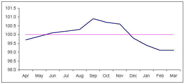
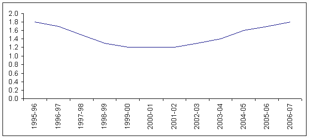
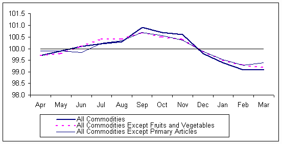
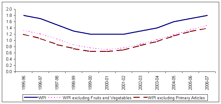
IV.2 Seasonal Adjustment IV.2.1 ILO's recommendations 4.7 The Consumer Price Index (CPI) continues to play an important role in national policy making, both in the economic and in the social sphere. It has been the long-standing tradition of the International Labour Office (ILO), the agency responsible for the subject of consumer price indexes within the UN system, to ensure the establishment of international standards on the topic. 4.8 The existence of seasonal commodities poses some significant challenges for price statisticians. Seasonal commodities are commodities which are either: (a) not available in the marketplace during certain seasons of the year, or (b) are available throughout the year, but there are regular fluctuations in prices or quantities that are synchronized with the season or the time of the year. A commodity that satisfies (a) is termed a strongly seasonal commodity, whereas a commodity that satisfies (b) is called a weakly seasonal commodity. It is strongly seasonal commodities that create the biggest problems for price statisticians in the context of producing a monthly or quarterly consumer price index (CPI) because if a commodity price is available in only one of the two months (or quarters) being compared, then obviously it is not possible to calculate a relative price for the commodity and traditional bilateral index number theory breaks down. 4.9 Chapter 22 of the ILO CPI manual (ILO et al., 2004) discusses the treatment of seasonal products in the CPI, and the problems posed by seasonal products in the calculation of the CPI. 4.10 Some important conclusions, indicated in this manual, are as follows: (i) Year-over-year inflation based on monthly indices can always be constructed even if there are strongly seasonal commodities. (ii) Rolling year indices give a reliable indicator of annual inflation at a monthly frequency. This type of index can be regarded as a seasonally adjusted CPI. It has the disadvantage of measuring year-over-year inflation with a lag of six months; hence it cannot be used as a short-run indicator of month-to-month inflation. 4.11 Annual basket indices can also be successfully used in the context of seasonal commodities. For commodity groups that have strong seasonality, an annual basket type index for this group can be seasonally adjusted and the resulting seasonally adjusted index value can be used as a price relative for the group at higher stages of aggregation. 4.12 The above analysis reveals that, as per international practices, inflation rate is widely presented year-on-year basis (based on deseasonalised price data), month-over-month basis (based on seasonally adjusted price data), etc. Thus, for appropriate assessment of emerging inflation during the year, it is essential to know the ‘extant’ and nature of seasonality prevailing in the price series (viz., WPI and CPIs) being used in India. Next section is devoted to examine these issues in detail. Seasonality in Price Measures: The Indian Case V.1 Nature of Seasonality 5.1 In this chapter, we examine the seasonal variations in the price indices, the WPI series taken at aggregate as well as disaggregate levels. The WPI-Fuel group is excluded from the disaggregate level analysis, because these prices are administered by the government. The reference period is from April 1994 to March 2007. The four CPI series are also taken into account of this analysis. The seasonal factors of the price indices are obtained by using the X-12-ARIMA methodology. V.1.1 Analysis on Wholesale Price Indices (WPI)3 V.1.1.1 Aggregate Level 5.2 The seasonal factors of WPI, at aggregate level, are given in Table 8. These seasonal factors are normalised around base 100, thus, whenever, seasonal factors exceeds 100, it represents the period, when prices are likely to show some upward shift, due to seasonal factors. Reverse results are likely to hold when seasonal factors are below 100. Results of Table 8 reveal that, during the period from 1995-96 to 2006-07, the WPI-All Commodities reveals very moderate seasonal variations. Although, the moving seasonality is noticed over the period, the seasonal peak and trough mostly occurred in the months of September, and February, respectively. The seasonal peak varied within 100.5 and 100.9, whereas, the trough varied within 98.9 and 99.3 (Chart 15). 5.3 The range of the seasonal factors, measuring the difference of peak and trough values, is incorporated, for evaluating the movement of seasonal fluctuations. The range of seasonal factors, for WPI-All Commodities, declined from 1.8 in 1995-96 to 1.2 in 2001-02, and increased subsequently. Over the reference period, this series has been showing a seasonal variability within a narrow band (Table 8 and Chart 16). Table 8: Seasonal Factors for WPI-All Commodities
5.4 Results of Chart 15 show that, price level in India, as based on WPI, is likely to have somewhat upward bias, due to seasonal factors, during the period August to November. Chart 15: Movement of Seasonal Factors of WPI-All Commodities during 2006-07
Chart 16: Range (Difference between Peak and Trough Values) of Seasonal Factors
V.1.1.2 Disaggregate Level 5.5 In case of aggregate level analysis of WPI series, the seasonal variation of WPI-All Commodities (WPI-AC) shows movement within a narrow band. Thus, it may be useful to know the seasonal variations at the disaggregated level. In this context, the two broad groups, viz., Primary Articles (PA), and Manufactured Products (MP); their sub-group levels, and commodity levels, are considered. The sub-groups and commodities are considered only if they have at least one per cent weight in aggregate. In addition, some of the sub-groups and commodities, viz., Pulses, Condiments and Spices, etc, are taken on judgmental basis. 5.6 Table 9 shows the 12-year average of seasonal factors of WPI at the aggregate and select disaggregate level, during the reference period. At the broad group level, the Primary Articles group shows higher seasonal fluctuations in prices, as compared to the Manufactured Products group. The seasonal fluctuations in the Primary Articles group are mainly due to the seasonal fluctuations in the Food Articles (FA) sub-group, both having seasonal trough in March, whereas their seasonal peaks occurred during October and November, respectively. The seasonal fluctuations of Foodgrains group is mainly dominated by the cereals group, both having seasonal peaks and troughs in the months of August and May, respectively. Table 9: Average of Seasonal factors of WPI - Aggregate and Selected Disaggregate level
5.7 During the reference period, the range of seasonal factors for Primary Articles was much higher, as compared to that of Manufactured Products. Within the Primary Articles group, the range of Food Products group declined. The Fruits and Vegetables group show highest seasonal fluctuations, though the range of seasonal factors for this group moderated from nearly 22.0 per cent to nearly 19.0 per cent over the years. Within the Manufactured Products group, the Food Products experienced high seasonal fluctuations (Table 10). Table 10: Range (Difference between Peak and Trough Values) of Seasonal factors of WPI
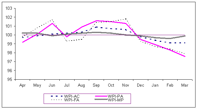
Chart 17: Movement of Seasonal Factors of WPI during 2006-07
5.8 Results of Chart 17 reveal that, seasonality in WPI, at aggregate level, and disaggregate level, is almost symmetrical in nature, though seasonality is much pronounced in case of Primary Articles, and expectedly very moderate in case of Manufactured Products. In both cases, the major sources of seasonality have been the food items (Food Articles, in case of Primary Articles, and Food Products, in case of Manufactured Products). 5.9 For a more detailed analysis of the sources seasonality, commodity wise data are used for the WPI basket. The seasonal variations of the series, over the period, are measured in terms of range of the seasonal factors, during the year. Based on this measure, the selected price series are classified in Table 11. Table 11: Range (Difference between Peak and Trough Values) of
5.10 It indicates that, the prices of Wheat, Oilseeds, Pulses, Fruits, and Vegetables show higher seasonal fluctuations, as compared to the other sub-groups and commodities. 5.11 Due to the high seasonal fluctuations in the Fruits and Vegetables group as witnessed in Table 10, a modified estimate of WPI-All Commodities is constructed by excluding this group, and the monthly seasonal factors, over the period, are extracted thereafter. The range of the seasonal factors of WPI is substantially reduced, once the Fruits and Vegetables are removed from the All Commodities Group (Table 12). Table 12: Peak, Trough and Range of Seasonal Factors for WPI-All Commodities
5.12 Similarly, the Primary Articles group is also excluded from the WPI-All Commodities group, and the seasonal factors of the new series are obtained. Chart 19 shows that, due to the exclusion of the Fruits and Vegetables group and Primary Articles group, from the All Commodities, the range of the seasonal factors becomes substantially low. 5.13 From the above analysis, it may be concluded that, food items, especially Fruits and Vegetables, are major sources of seasonal fluctuations in WPI. It needs to be mentioned here that, for some commodities, under fruits and vegetables, the weights are distributed among remaining items under the group, as no price quotations are available. These may also be a major source of seasonality inbuilt in construction of the index. Since food items are larger share in CPI, they are bound to introduce strong seasonality in CPIs too which is analysed in next section. Chart 19: Range (Difference between Peak and Trough Values) of Seasonal Factors
V.1.2 Analysis on Consumer Price Indices (CPI) 5.14 In order to analyze the seasonal behaviour of the consumer price series, four series, viz., CPI – Industrial Workers, Agricultural Labourers, Rural Labourers, and Urban Non-Manual Employees, are considered. Over the reference period, the seasonal peak of all the four CPI series varied over October and November, while the seasonal trough varied over March and April (Table 13). Table 13: Average of Seasonal factors of CPI
5.15 The range of seasonal factors of CPI-Industrial workers decreased steadily from 1997-98 to 2004-05, and then increased in the last two years. Similar movements were also noticed in the case of CPI-Agricultural Labourer and Rural Labourer. On the other hand, the CPI-Urban Non-Manual Employees showed a steady decrease in the range, during the reference period (Table 14). Over the reference period, the seasonal variations of CPI-Industrial Workers continued to be higher than that of WPI-All Commodities. The degree of divergence in the seasonal variations of the two series narrowed in the recent period, although indications of marginal widening of the gap are visible. Table 14: Range (Difference between Peak and Trough Values) of Seasonal factors of CPI
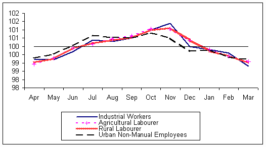
Chart 20: Movements of Seasonal Factors of CPI during 2006-07
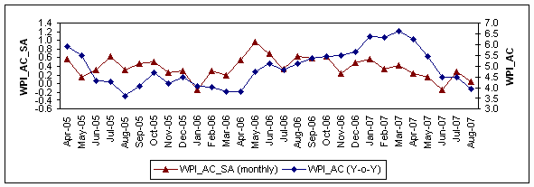
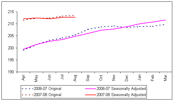
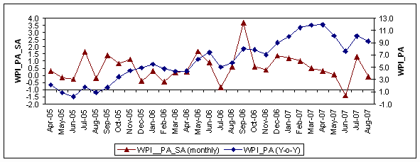
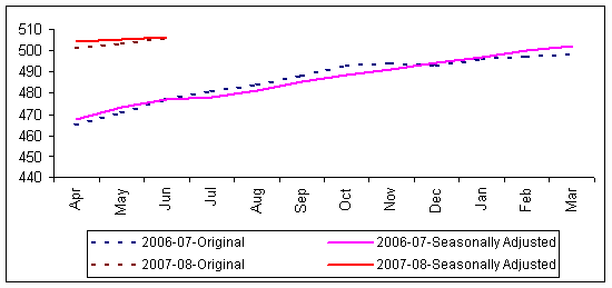
5.16 Chart 20 reveals that, level of seasonality is much stronger in case of all CPI series relative to WPI, due to high weight of food items in CPI basket, as compare to WPI. In terms of incidence during the year (i.e., peak/trough), it turned out to be similar to WPI. V.1.3 Movements of variations in Original and Seasonally Adjusted Series 5.17 The analysis of the monthly variations in the seasonally adjusted WPI series throws some light on the price dynamics in the economy. This analysis augments the other regular analysis carried out using the year-on-year variations in the unadjusted data. In this section, monthly variations in seasonally adjusted WPI series are compared with the year-on-year variations in the unadjusted WPI series through graphical analysis. The monthly variations in the WPI – All Commodities series show that there has been visible deceleration during April 2007 to August 2007, except for the month of July 2007 (Chart 21). Similar movements are also observed in the case of year-on-year variations in the WPI series. Chart 21: Variations in WPI All Commodities – Apr-2005 to Aug-2007
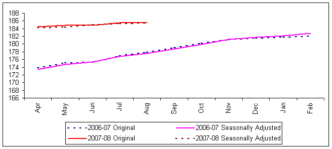
5.18 Chart 22 shows the movements of original and seasonally adjusted WPI-All Commodities. Since WPI-All Commodities exhibit low seasonal fluctuations, this is supplemented with disaggregate level analysis. Chart 22: WPI-All Commodities – Original and Seasonally Adjusted
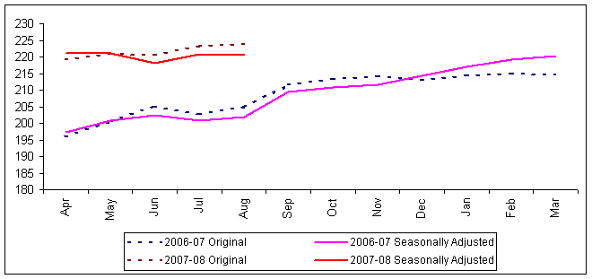
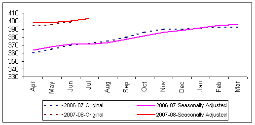
5.19 The year-on-year variations in WPI – Primary Articles showed a continued up thrust till April 2007, then a fall observed for the two months, viz., May and June 2007 (Chart 23). For the last two months, there were fluctuations in the inflation rates. The monthly movements in the seasonally adjusted series, however, had already reflected that WPI – Primary Articles had started decelerating from January 2007 onwards. For the last two months, viz., July and August 2007, similar movements, as compared to annualized inflation rates, were observed. Chart 24: WPI-Primary Articles – Original and Seasonally Adjusted
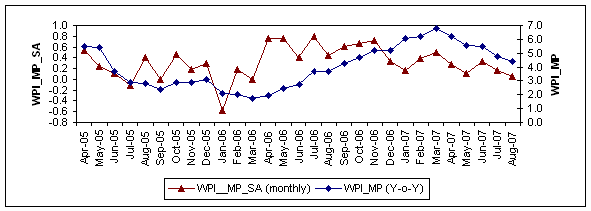
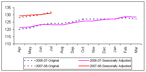
5.20 Among the WPI major groups, WPI – Manufactured Products is least seasonal in nature. The year-on-year variations show a steep rise in this series from March 2006 onwards (Chart 25). The deceleration in the series is observed from April 2007. On the other hand, the monthly variations in the seasonally adjusted series showed a sharp rise from January 2006 to November 2006. During the period of December 2006 to August 2007, although the monthly variations in the seasonally adjusted series show more fluctuations, as compared to year-on-year variations of the original series, there is a decelerating movement of these variations. Chart 25: Variations in WPI Manufactured Products – Apr-2005 to Aug-2007 Chart 26: WPI-Manufactured Products – Original and Seasonally Adjusted
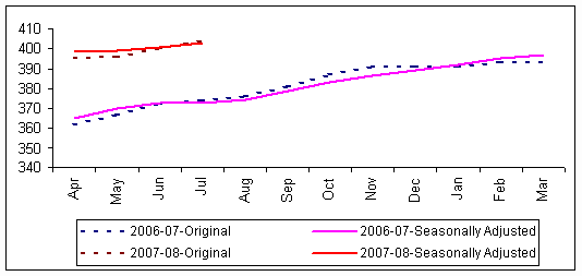
5.21 Chart 24 and Chart 26 give the original and seasonally adjusted series for WPI – Primary Articles and Manufactured Products, respectively. It may be noted that, between the two broad groups of commodities, viz., Primary Articles, and Manufactured Products, the WPI of Primary Articles group is more seasonal in nature. 5.22 In order to analyze the seasonal nature of the CPI series, the seasonally adjusted data of the four series, viz., CPI- Agricultural Labourers, Industrial Workers, Rural Labourers, and Urban Non-Manual Employees, are compared with the original series. Charts 27 to 30 represent the movements of original and seasonally adjusted CPI series, from April 2006 onwards. Chart 27: CPI-Agricultural Labourers – Original and Seasonally Adjusted
Chart 28: CPI-Industrial Workers – Original and Seasonally Adjusted
Chart 29: CPI-Rural Labourers – Original and Seasonally Adjusted
Chart 30: CPI-Urban Non-Manual Employees – Original and Seasonally Adjusted
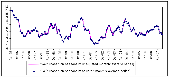
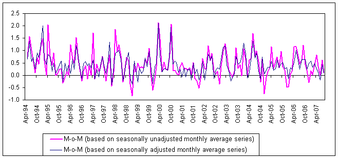
V.2 Remarks 5.23 Chart 22 indicates that, the year-on-year inflation rate, measured for both seasonally adjusted and unadjusted data, are same. For example, the year-on-year inflation rate has been worked out using seasonally adjusted and unadjusted data for April 1995 to August 2007. These results, as expected, reveal no difference between year-on-year inflation based on seasonally adjusted versus seasonally unadjusted data. On the other hand, the inflations, measured during the year, both for seasonally adjusted and unadjusted data, show differences, due to seasonal fluctuations (Chart 31 and Chart 32). Similarly, analysis holds good for CPI series, as well. Chart 31: Year-on-Year Inflation Rate based on Seasonally Adjusted and
Chart 32: Month-over-Month Inflation Rate based on Seasonally Adjusted and
5.24 Results of this chapter reveal that, all price series (viz., WPI and CPI) in India exhibit certain level of seasonal fluctuation during the year. Thus, for any analysis of price dynamics pertaining during the year, seasonal adjustment would be essential. However, for annual point-to-point comparison, seasonal adjustments of price series are irrelevant. Many a times, signal emerging from annual point-to-point inflation rate and based on variation during the year, may not be identical. In the next section, certain such episodes are discussed, before the concluding remarks and recommendations. Comparative Analysis of Different Inflation Measures 6.1 Chapter II discusses the measurement issues of the inflation rate. In India, the annual point-to-point inflation rate is generally disseminated and is widely used. But this measure suffers from the limitation that, it confounds the movements in the current year's WPI with the base effect. There have been instances when annual point-to-point inflation does not reveal the true picture of the inflationary pressure in the economy. In order to assess the true signal of inflation, year-on-year, measures based on moving averages, month-over-month, fixed base methods are also discussed. Monthly/Quarterly movements of WPI are affected by the seasonal fluctuations. Therefore, these indices are required to be deseasonalised. In this respect, X-12-ARIMA procedure (a widely used statistical technique developed by the US Census Bureau) is adopted. 6.2 It was observed that, during the recent period, in October 2006 to January 2007, there was no rise in WPI, but annual point-to-point inflation rate increased from 5.3 per cent to 6.7 per cent (Table 15). Table 15: Annual Inflation based on Point-to-Point Measure
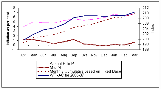
6.3 Thus, as it reflects from Table 15, the annual inflation rate, measured on annual point-to-point basis, sometimes gives misleading signal regarding the actual price movement during the year. Table 16: Measures of Inflation for 2006-07
# Annualised inflation for the month is obtained by the formula given below, Annual inflation = (Monthly Cumulative based on Fixed Base) X 12÷(No. of months Cumulated) Chart 33: Movement of Selected Inflation Presentations
6.4 During the year, the monthly cumulative inflation, based on fixed base method, has movement similar to the WPI movement (Table 16 and Chart 33). 6.5 The analysis reveals that, the annual point-to-point inflation, supplemented with the movements of month-over-month inflation and fixed base inflation, provides a clearer and comprehensive view of the inflation dynamics in the Indian economy. Conclusions and Recommendations 7.1 Communication of inflation rate appropriately is important, as economic agents and financial markets are expected to form their price expectations based on official published figures. Publication of inflation figures, not consistent with actual movements in price series, i.e., WPI/CPI, may result in formation of biased expectations. 7.2 In general, inflation rate is presented as variation in price indices with respect to a previous period, such as, annual point-to-point, month-over-month, etc. In the Indian context, official inflation rate is measured based on annual point-to-point basis change in the Wholesale Price Index (WPI). Measurement of inflation rate based on annual changes in prices or annualisation of changes over shorter period (month/quarter) is necessary for relating inflation with financial indicators (e.g., interest rates). 7.3 Analysis of annual point-to-point inflation reveals that, these are susceptible to the base effect. An alternative method of measuring inflation could be month-over-month variation in WPI, using seasonally adjusted data. However, such inflation rate exhibits high volatility, and does not exhibit appropriate stable signals about price changes. Measuring inflation i.e., price variation over a fixed base (say, end-March data of the previous financial year), also provides useful information regarding price dynamics during the year. These measures of inflation, though appropriate for assessing inflation during the year, have limitations, as they do not provide (appropriate) annualised inflation rates. 7.4 Similarly, annual inflation rates worked out on the basis of moving average of price indices of previous 4/12/52 weeks exhibit lower variability due to increased smoothening and captures almost all the important turning points by reducing noise elements. However, it is biased towards past data and has a centre, which becomes increasingly remote as the length of observations considered increases. Such measures of inflation rate become less useful for measuring current (underlying) inflation. 7.5 Internationally, the most common method of inflation measurement is the annual point-to-point change in consumer price index, though annualised variations over shorter horizon are also used. For example, Bank of England, in its Inflation Report, presents inflation rate, based on the annual percentage change, for each month of the year. Similarly, European Central Bank presents the inflation rate, based on annual percentage change on monthly data. Bank of Japan presents annualised, as well as monthly inflation rates, for each month of the year. In many of the Central Banks, the month-over-month inflation rate is obtained, using seasonally adjusted data. 7.6 In the Indian context, X-12-ARIMA and its earlier variants, which are also used by the Bureau of Labour Statistics (BLS), USA, have been used since 1980, for obtaining seasonal adjustment in price data. A detailed analysis, as carried out by the Group, found that, seasonal factors of WPI and CPI series, obtained by using X-12-ARIMA procedure, reveal that prices firms during the period August – November. Incidentally, this period encompasses occurrence of monsoon, when there could be supply bottlenecks, and festival seasons when there could be demand escalation. These results appear to be consistent with expected price changes during the year, on account of seasonal factors. Thus, X-12-ARIMA appears to be appropriate for seasonal adjustment of WPI and CPI series during the year. 7.7 All the price series in India (viz., WPI, CPI) have peak/trough months around same time of the year mainly due to seasonality in food prices, which are the major source of seasonality in all price indices. Generally, price level (not inflation rate) is likely to show upward bias during August-November, whereas, for the remaining months, the price level should show the downward bias. Seasonality is more profound in various CPIs as compared to WPI. Although the impact of seasonality is much pronounced in prices of Fruits and Vegetables; relatively moderate seasonality in some foodgrains, viz., Wheat, Pulses, etc., also influence the seasonal behaviour of aggregate price index due to their high weights. Excluding these commodities, the degree of changes in WPI, due to seasonality, is relatively low. Seasonality in Manufactured Products is very low and emanates from price changes for Food Products. 7.8 Finally, the analysis revealed that, inflation rate based on annual point-to-point basis, supplemented with month-over-month and fixed base (using seasonally adjusted price series) provide better signal regarding price dynamics in the Indian economy.
Seasonal Adjustment: Description of the Methods TRAMO/SEATS The TRAMO/SEATS program runs through the following steps: 1. First an ARIMA model is identified automatically by TRAMO. 2. At the same time outliers are identified automatically (if necessary TRAMO calculates other regression variables such as trading days or Easter variables). 3. TRAMO passes the linearized series to SEATS, where the actual decomposition is done. 4. In SEATS, first the spectral density function of the estimated model is decomposed into the spectral density function of the unobserved components, which are assumed to be orthogonal. As in the other methods, assumptions have to be made to get an estimator. The assumptions made are listed in the synopsis overleaf. 5. Then SEATS estimates the parameters of the two components (trend-cycle and seasonally adjusted component). Since for this the Wiener-Kolmogorov filter is used, the observed series have to be forecasted and backcasted. 6. Finally the outlier- and special effects are reintroduced into the components. TRAMO can handle four types of outliers, viz., level shift, additive outlier, temporary change, and, innovation outliers. It can also estimate the calendar effects as well as missing observations and regression effects. The order of the different parameter for the ARIMA model is constrained to the following range for SEATS: a) Order of autoregressive polynomial: P £ 3 b) Order of differencing: D £ 3 c) Order of moving average polynomial: Q £ 3 d) Order of seasonal autoregressive polynomial: BP £ 1 e) Order of seasonal differencing: BD £ 2 f) Order of seasonal moving average: BQ £ 1 and the constraint g) P+D+BP x (Number of observations per year) + BD x (Number of observations per year) ³ Q + BQ x (Number of observations per year) SEATS offers many analytical tools, which give the basis of statistical inference including errors of the component estimator, forecast errors, Ljung Box test and Box Pierce test for the adequacy of the ARIMA modelling. Several graphical tools are offered such as graphs for the spectra for the components, filter gains and autocorrelation function of the residuals. The most important difference to the ad-hoc methods is the basis of statistical inference and the adaptive filters of SEATS, which adapts to the modelled characteristics of the time series. These advantages are of course only valid, if it is possible to model the time series adequately. X-11/X-12-ARIMA The CENSUS X-11 method is a seasonal adjustment method based on different kinds of moving averages without an underlying explicit model and it was developed mostly on an empirical basis. In the default option, it uses ratio to moving average methods, a multiplicative relationship between the components is assumed but it has also an option to handle additive and log additive models. The method tested was the X-11-ARIMA/88 method from Statistics Canada (see Dagum 1988). At first the method X-11 will be described and then the differences to X-11-ARIMA/88 and reasons why to incorporate X-11-ARIMA/88 instead of X-11 are given. The method is based on symmetric moving averages, at the end asymmetric filters must be used with less preferable characteristics. The different steps can be described (according to Dagum (1988)) in the following way: 1. Compute the ratios between the original series and a centred 12-term moving average as the first estimate of the seasonal and irregular component (St Î t); 2. Apply a weighted 5-term moving average (3x3 moving average) to the seasonal-irregular ratios (St Î t) of each month separately, to obtain a preliminary estimate of the seasonal factors; 3. Compute a centred 12-term moving average of the preliminary factors found in step 2 for the entire series. To obtain the six missing values at either end of this average, repeat the first (last) available moving average value six times. Adjust the factors to add to 12 (approximately) over any 12-month period by dividing the centred 12-term average into the factors to get a preliminary estimate for the trend-cycle; 4. Divide the seasonal factor estimates into the seasonal irregular (St Î t) ratios to obtain an estimate of the irregular component; 5. Outlier detection: Compute a moving five-year standard deviation (s ) of the estimates of the irregular component and test the irregulars in the central year of the five-year period against 2.5s . Remove values beyond 2.5s as extremes and recompute the moving five years. Assign a zero weight to irregulars beyond 2.5s and a weight of 1 to irregulars within 1.5s . Assign a linearly graduated weight between 0 and 1 to irregulars between 1.5 and 2.5s ; 6. For the first two years, the limits, computed for the third years are used, and for the last two years, the limits computed for the third last years are use. To replace an extreme ratio in either the two beginning or ending years, the average of the ratio times its weight and the three nearest full weight ratios for that month are taken; 7. Apply a weighted 5 term moving average to the St Î t ratios with extreme values replaced, for each month separately, to estimate preliminary seasonal factors; 8. Repeat step 3, applied to the factors found in step 7; 9. Divide the output in step 8 into the original series to obtain a preliminary seasonally adjusted series; 10. Apply a 9-, 13- or 23-term Henderson moving average to the seasonally adjusted series and divide the resulting trend cycle into the original series to give a second estimate of the St Î t ratios (in the first iteration, only the 13 term Henderson is applied.); 11. Apply a weighted 7-term moving average (3x5 moving average) to each months St Î t ratios separately, to obtain a second estimate of the seasonal component; 12. Repeat step 3; 13. Divide the output from step 11 into the original series to obtain the seasonally adjusted series. The advantages of X-11 are 1. Robustness, The disadvantages are: 1. Use of asymmetric filter at both ends of the time series, One disadvantage, the asymmetric filters, led to the development of X-11-ARIMA/88 (see Dagum 88), which uses ARIMA forecasts and backcasts to prolong the time series with values for one year. After the prolongation of the time series, only a less asymmetric filter has to be used, the amount of revisions is as shown in several empirical comparisons (see for example Dagum (1988) much smaller than in X-11. For the ARIMA modelling of the time series the following models were chosen: For the multiplicative model and the log additive model: log(0,1,1)(0,1,1)s , log (0,2,2)(0,1,1)s, and (2,1,2)(0,1,1). For the additive model: (0,1,1)(0,1,1)s , (0,2,2)(0,1,1)s and (2,1,2)(0,1,1)s. The ARIMA model notation used is the classical notation of Box Jenkins (1970) ARIMA(p,d,q)(P,D,Q)s where p and P denote the number of ordinary and seasonal auto regressive parameters, q and Q denote the number of the ordinary and the seasonal moving average parameters respectively, d and D denote the degree of the ordinary and the seasonal differences respectively. X-12 ARIMA is an enhanced version of the X-11 Variant of the Census Method II seasonal adjustment programme. The procedure makes multiplicative/additive adjustments of a time series and creates an output data set containing the adjusted time series and intermediate calculations. The main source of these new tools is the extensive set of time series model building facilities built into the programme for fitting the regARIMA models. The regARIMA-modeling module of X-12-ARIMA was adopted from the regARIMA programme developed by the Time Series Staff of Census Bureau's Statistical Research Division. A fundamentally important use of regARIMA models is to extend the series with forecasts (and backcasts) in order to improve the seasonal adjustments of the most recent (and the earliest) data. Doing this mitigates problems inherent in the trend estimation and asymmetric seasonal averaging processes of the type used by the X-11 method near the ends of the series. The provision of this extension was the most technical improvement offered by Statistics Canada’s widely used X-11-ARIMA programme. Plans for X-12-ARIMA developed around the operation-flow diagram of Figure 1. This posits a regARIMA (linear regression model with ARIMA time series errors) modeling subprogram that can provide forecasts, backcasts, and prior adjustments for various effects before the seasonal adjustment subprogram in the central box is invoked. The final box in Figure 1 represents a set of post-adjustment diagnostic routines that can be used to obtain indicators of the effectiveness of both the modeling and the seasonal adjustment options chosen. The modeling module of X-12-ARIMA is designed for regARIMA model building with seasonal economic time series. To this end, several categories of predefined regression variables are available in X-12-ARIMA (for further details user may refer to the manual available at 'htttp://www.census.gov/srd/www/x12a/'). User-defined regression variables can also be easily read in and included in models. X-12-ARIMA also uses the standard (p d q) (P D Q)s notation for seasonal ARIMA models. Great flexibility is allowed in the specification of the ARIMA structures: any number of AR, MA, and differencing operators may be used; missing lags are allowed in AR and MA operators; and AR and MA parameters can be fixed at user-specified values. The specification of a regARIMA model requires specification both of regression variables to be included in the model and also the type of ARIMA model for regression errors (i.e., the orders (p d q) (P D Q)s). Specification of the regression variables depends on user knowledge about the series being modelled. Figure 1: Flow Diagram for Seasonal Adjustment with X-12-ARIMA 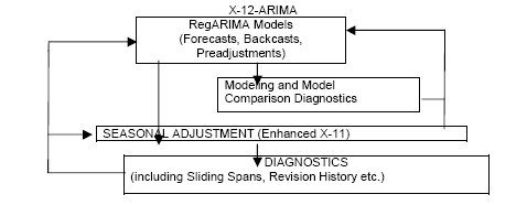
For the user who wishes to fit customised time series models, X-12-ARIMA provides capabilities for the three modeling stages of identification, estimation, and diagnostic checking. Identification of the ARIMA model for the regression errors follows well-established procedures based on examination of various sample autocorrelation and partial autocorrelation functions produced by X-12-ARIMA. Once a regARIMA model has been specified, X-12-ARIMA will estimate its parameters by maximum likelihood using an iterative generalised least squares (IGLS) algorithm. Diagnostic checking involves estimation of residuals from the fitted model for signs of model inadequacy. The major improvements in X-12 ARIMA are new modeling capabilities using regARIMA models, sliding spans diagnostic procedure, ability to produce revisions history of a given seasonal adjustment, several new outlier detection options for the irregular component of the seasonal adjustment etc. RegARIMA RegARIMA is a linear regression model with ARIMA that can provide forecasts and prior adjustments for various effects. X-12 ARIMA uses regARIMA models to preadjust a series by removing effects such as outliers, etc., before the seasonal adjustment program is invoked. Let B denote the backshift operator, Byt = yt-1. X-12-ARIMA can estimate regARIMA models of order (p d q)(P D Q) s for yt. These are models of the form
(2) where 's' is the length of the seasonal period, s = 4 or 12. The polynomials Φp(z), F P(z), q q(z), Q Q(z) with degrees p; P; q; and Q respectively have constant terms equal to one. These polynomials are constrained so that the zeroes of q q(z) and Q Q(z) have magnitudes greater than or equal to one, so that the zeroes of Φp(z) and F P(z) have magnitudes greater than one. Because 'at' is assumed to be a sequence of independent variables with mean '0' and constant variance s a2 , it follows from these constraints that
(3) is a covariance stationary time series that satisfies the difference equation
(4) Consequently, we can re-express the model (3) for yt as,
(5) This is a regression model with stationary ARMA errors wt for suitably differenced yt. Its regressors result from applying the same differencing operations to the xit. The model (6), together with an assumption that the innovations at in the model for wt are i.i.d N(0, σ2 ), determine the likelihood function that is maximized to estimate the regression coefficients b i , σ2 and the coefficients of Φp (B), F P (Bs), q q (B), and Q Q (Bs). The default likelihood in X-12-ARIMA is the fully exact Gaussian likelihood. In model estimation, any of the ARMA coefficients can be held at fixed values, such as zero. The program produces asymptotic standards errors, correlations, and t-statistics for the estimated coefficients as well as confidence intervals for forecasts. Following are the different types of regressors used in RegARIMA: 1) Constant term (for stationary variable i.e., if the ARIMA model does not use differencing) represents the mean of the (stationary) series provided there are no other regression variables in the model. 2) Trend term captures the deterministic trend present in the data. The polynomial trend term reduces to a constant term after differencing. 3) Fixed seasonal regressors can be in one of the following category: a) 11 contrasts in the 12 indicator variables. b) 11 variables taken from the Fourier series representation of a fixed monthly pattern. 4) X-12 ARIMA provides four other types of regression variables to deal with abrupt changes in the level of a series of a temporary or permanent nature: additive outliers (AOs), level shifts (LSs), temporary changes (TCs) and ramps. AOs affect only one observation in the whole series and hence this effect is removed by a dummy variable, which takes '0' at break and '1' for other period. LSs increases or decreases all observations from a certain time point onward by some constant amount, this LS effect is removed by introducing a dummy variable which takes value '-1' for all the time point up-to the break point and '0' for all the time points afterwards. TCs allow for an abrupt increase or decrease in the level of the series that returns to its previous level exponentially, this effect is captured by a variable which takes value '0' for all observation before the change point and a t (O<a <l) Adam K., Padula M., 2003, 'Inflation Dynamics and Subjective Expectations in the United States', Working Paper No. 222, European Central Bank Bank of England, Inflation Report, August 2007. Bank of Jamaica, Quarterly Monetary Policy Report, October – December 2006. Bank of Japan, Quarterly Bulletin, November 2006. Bank of Thailand, Inflation Reports, July 2007. Bell W. R., Hillmer S. C., 1992, 'Forecasting, Methods and Applications', 2nd Ed., Makridakis, Wheelwright and McGee. Bell, W. R., 1992, 'X-12 Time Series Modelling Course', US Bureau of Census concept paper,Washington. Blinder A., Goodhart C., Hildebrand P., Lipton D., Wyplosz C., How Do Central Banks Talk?, 2001, Geneva Reports on the World Economy 3, International Centre for Monetary and Banking Studies. Bryan M. F., Cecchetti S. G., 1995, 'The Seasonality of Consumer Prices,' NBER Working Papers 5173, National Bureau of Economic Research, Inc. Burman J.P., 1980, Seasonal adjustment by signal extraction. Journal of the Royal Statistical Society, Series A 143, pp. 321–337. Central Bank and Financial Services Authority of Ireland, Quarterly Bulletin, July 2007. Central Bank of Norway, Inflation Report with Monetary Policy Assessments, November 2004. Deutsche Bundesbank, Monthly Report, July 2007. European Central Bank, Monthly Bulletin, August 2007. Forsells M., Kenny G., 2002, 'The rationality of Consumers' Inflation Expectations: Survey-based Evidence for Euro Area', Working Paper No. 163, European Central Bank Hogan s., Johnson M., Lafleche T., 2001, Core Inflation, Bank of Canada, Technical Report No. 89. International Labour Office, 2004, Consumer Price Index Manual, Chapter 22, pp. 393 – 417. Macauly, F.R., 1931, The Smoothing of Time Series, New York: National Bureau of Economic Research. U.S. Census Bureau, 'X-12-ARIMA Reference Manual', version 0.2.8. Reserve Bank of Australia, Quarterly Statistical Release, October 24, 2007. United States Census Bureau, 2001, X-12-ARIMA Reference Manual, version 0.2.8. United States Department of Labour, Bureau of Labour Statistics, News, October 2007. |
|||||||||||||||||||||||||||||||||||||||||||||||||||||||||||||||||||||||||||||||||||||||||||||||||||||||||||||||||||||||||||||||||||||||||||||||||||||||||||||||||||||||||||||||||||||||||||||||||||||||||||||||||||||||||||||||||||||||||||||||||||||||||||||||||||||||||||||||||||||||||||||||||||||||||||||||||||||||||||||||||||||||||||||||||||||||||||||||||||||||||||||||||||||||||||||||||||||||||||||||||||||||||||||||||||||||||||||||||||||||||||||||||||||||||||||||||||||||||||||||||||||||||||||||||||||||||||||||||||||||||||||||||||||||||||||||||||||||||||||||||||||||||||||||||||||||||||||||||||||||||||||||||||||||||||||||||||||||||||||||||||||||||||||||||||||||||||||||||||||||||||||||||||||||||||||||||||||||||||||||||||||||||||||||||||||||||||||||||||||||||||||||||||||||||||||||||||||||||||||||||||||||||||||||||||||||||||||||||||||||||||||||||||||||||||||||||||||||||||||||||||||||||||||||||||||||||||||||||||||||||||||||||||||||||||||||||||||||||||||||||||||||||||||||||||||||||||||||||||||||
صفحے پر آخری اپ ڈیٹ:


