 IST,
IST,


Monetary Policy Report - September 2015
Macroeconomic developments in the first half of 2015-16 have evolved in close alignment with baseline forecasts. Going forward, inflation is projected to stay below the January 2016 target in 2015-16 and ease further in 2016- 17. The projection of growth is revised downward for 2015-16, with some firming in the following year. Potential volatility in global financial markets poses the most significant risk to these projections. Over the first half of 2015-16 (April-March), macroeconomic developments have evolved in close consonance with staff’s baseline forecast paths set out in the April 2015 Monetary Policy Report (MPR). Deviations in levels, albeit small, are observed both above and below the projections, indicating the absence of systematic bias in forecast errors. Chapters II and III explain the factors underlying these deviations in inflation and growth developments, respectively. Significant shifts in global and domestic macroeconomic and financial conditions since the April 2015 MPR warrant a re-assessment of the baseline assumptions determining the initial conditions that drive staff’s projections, and revisions if any (Chart I.1). First, from the second quarter (Q2) of 2015-16, international crude oil prices have fallen substantially below the April 2015 MPR baseline assumption1. The lower level of oil prices assuaged domestic inflation pressures, supported domestic demand and helped to contain fiscal and current account deficits. Secondly, notwithstanding some bright spots – mainly the US and the Euro area – global growth has weakened below expectations, and the deepening slowdown in emerging and developing economies (EDEs) could warrant downward revisions in forecasts (Table I.1). Thirdly, high volatility seems to have become the new normal in global financial markets, with sharp risk-onrisk- off swings shifting external financial conditions across the emerging world. Prominent triggers are concerns about China - growth slowdown; stock market meltdown; devaluation - as well as the pace and timing of interest rate action by the US Federal Reserve. Fourthly, the growth in volume of world trade is hovering below the growth of the world GDP, vitiating the underlying price and income elasticities and weakening the contribution of exports to aggregate demand for a broad swathe of economies, advanced and emerging alike. With international trade prices contracting faster than trade volumes, the differential effects of terms of trade movements on net commodity exporters and importers have become somewhat blurred. Overall, global risks have heightened significantly. Domestically, the full impact of the deficient and spatially uneven south-west monsoon is still unfolding. Staff’s growth and inflation projections for eight quarters ahead in the MPR are generated out of three interacting and mutually reinforcing models: (a) a macro econometric model that simulates the working of the economy and estimates structural parameters; (b) a forecasting and policy analysis system (FPAS) that uses these structural parameters to generate alternative paths of the policy interest rate under various shocks comprising the balance of risks (Box I.1), using two quarters ahead projection of key variables obtained from (c) a full information projection system that employs competing models (structural time-series analysis; multivariate regression analysis; forward looking surveys and lead indicators) aggregated parsimoniously through root mean squared error (RMSE) scores. Inflation expectations play a critical role in the formation of inflation through their impact on wage and price contracts. In the September 2015 round of the Reserve Bank’s survey, urban households have reported a firming up of their inflation expectations, one quarter as well as one year ahead, for the third consecutive quarter (Chart I.2). Qualified by the caveat that the Reserve Bank’s survey has yielded only 41 observations so far2, there is strengthening empirical evidence of a significant element of backwardlookingness in households’ inflation expectations with high sensitivity and adaption to recent movements in a few salient prices such as those of vegetables, fruits and petrol. Inflation expectations also reflect the memory of close to double digit inflation for six years (up to 2013-14). The September round of the survey indicates that inflation is expected to be 10.5 per cent in Q3 and 10.8 per cent one year ahead. Professional forecasters expect short-run inflation to pick up in the coming quarters, in consonance with staff’s projections (Chart I.3). Importantly, their inflation expectations 10 years ahead moderated to 4.7 per cent in the September 2015 survey, approaching the Reserve Bank’s medium-term target, and indicating a better anchoring of long-term inflation expectations. Purchasing managers’ indices (PMI) indicate softening of inflationary pressures to their weakest level since April with upside pressures from the services sector being more than offset by the downside pressures from the manufacturing sector. Manufacturers polled by the Reserve Bank’s industrial outlook survey expect increases in output prices to moderate, driven down by lower input prices as also weakening pricing power (Chart I.4). Inflationary pressures from rural wage growth have remained relatively muted on the back of a moderation in nominal wage growth and going forward, they are expected to remain contained. Box I.1: Forecasting and Policy Analysis System Central banks adopting flexible inflation targeting have favoured the development of a forward-looking monetary policy framework centred on inflation forecasts as intermediate targets. A forecasting and policy analysis system (FPAS) has found appeal in terms of generating consistent model-based forecasts of the economy and calibrating policy reactions. The core of the FPAS is a quarterly projection model (QPM), which is a forward-looking open economy calibrated general equilibrium gap model in the new Keynesian tradition (Berg et al, 2006). Satellite models augment QPM by providing sectoral dynamics. The QPM consists of four blocks: (a) an aggregate demand or IS function; (b) an inflation block capturing food, fuel, and core (excluding food and fuel) inflation dynamics, the last element taking the form of a hybrid New Keynesian Phillips curve; (c) the exchange rate block; and (d) a forward looking policy reaction function. In real life, both inflation and growth are subject to considerable volatility and this affects public welfare adversely by imposing uncertainty around decision-making. Optimal monetary policy is all about maximising the well-being of economic agents in the country. In its simplest form, it can be described in terms of two components: one, minimising the deviations of inflation from a certain optimal rate and two, minimising deviations of real economic activity from the level determined by the productive potential of the economy. Setting optimal policy requires the assignment of optimal weights to each, depending on the responsiveness of demand to the real interest rate and the sensitivity of inflation to marginal cost and supply shocks. The optimal policy response will vary according to the size of these weights and the speed with which the policy instrument (the interest rate) is adjusted. Estimates of an optimal monetary policy rule in a FPAStype framework indicate that for India, the optimum weight on the inflation gap (actual minus target) ranges between 1.6 and 2.2, while the weight on the output gap (actual minus potential) varies between 0.8 and 1.4, with these weights increasing as the speed of adjustment of the policy repo rate rises (the interest rate smoothing parameter falls). References: Berg, A., P. Karam, and D. Laxton (2006), “A Practical Model-based Approach to Monetary Policy Analysis: Overview”. Working Paper No. WP/06/80, International Monetary Fund. Patra, M.D., J.K. Khundrakpam, and S. Gangadaran (2015), “Optimal Simple Monetary Policy Rules for India with New CPI Inflation as the Nominal Anchor”, (Mimeo). Headline CPI inflation is expected to firm up from its current trough and rise to around 4.5 per cent in September as favourable base effects reverse and average 5.5 per cent in Q3 and 5.8 per cent in Q4 of 2015-16. Assuming that various determinants of inflation evolve in the manner posited by staff in this MPR, especially the evolution of global crude oil and domestic food price dynamics, CPI inflation is expected to average 5.5 per cent in 2016-17 and moderate to around 4.8 per cent in Q4 of 2016-17 (with a 70 per cent confidence interval of 2.6-7.0 per cent) (Chart I.5). The baseline outlook, however, is subject to considerable uncertainties surrounding commodity prices, monsoon and weather-related disturbances, volatility in seasonal items and spillovers from external developments through exchange rate and asset price channels (Box I.2). A factor complicating forecasts of real gross value added (GVA) is the underlying behaviour of deflators of various types of economic activity (Chapter II, Box II.3). Looking ahead, the macroeconomic environment appears subdued. While consumption demand seems to be holding up other than in rural areas, the outlook for investment demand remains lacklustre with a shrinking pipeline of greenfield projects, lack of forward movement on the brownfield pipeline, the pressure of considerable slack as evident in persisting under-utilisation of capacity and build-up of finished goods inventories, still high stress on banks’ balance sheets and limited progress on major structural reforms. The prospects for exports too appear muted in view of the deterioration in the external trading environment. Moreover, the gains in terms of real incomes expected from favourable terms of trade for net commodity importers have been weak so far. Over the second half of 2015-16, the recovery in the agricultural sector observed in Q1 is unlikely to sustain, given the 14 per cent deficit in rainfall as well as its uneven distribution, and lower reservoir levels. The industrial sector continues to suffer from structural weakness in various core sectors: financial stress among distribution companies (DISCOMs) in the electricity sector, declining natural gas and crude oil production, coal production impacted by weak demand, and sharp fall in international steel prices affecting domestic producers. Overall consumer confidence polled in the September 2015 round of the Reserve Bank’s survey ebbed with regard to prospects for income and employment (Chart I.6). Box I.2: Central Bank Forecasts Timely and accurate forecasts of growth and inflation play a critical role in the conduct and formulation of monetary policy. If the assumptions underlying these forecasts undergo drastic changes, actual outcomes may deviate substantially from the initial forecasts. A survey of 16 central banks indicates that 13 overpredicted inflation during 2014 by an average of about 150 basis points (bps)@ (Chart a), driven by large unexpected declines in crude oil and other commodity prices. An optimism in growth projections is also evident in 2014, with average over-prediction of around 30 bps# (Chart b). This optimism is also visible in the IMF’s growth forecasts for 2011-14 which were, on average, 60 bps more than actual growth, with average forecast errors for EDEs being almost twice as large as those for AEs (IMF, 2014). In India, actual growth in 2014 was higher than projected, largely an outcome of the revised methodology under the new GDP series. Given the uncertainty in the evolution of baseline assumptions, therefore, many central banks encompass their point forecasts for inflation and growth within fan charts, which provide a probabilistic assessment of the likely outcomes for inflation and growth. Reference: International Monetary Fund (2014), World Economic Outlook, October. Business conditions assessed in the September 2015 round of the Reserve Bank’s industrial outlook survey were slanted to the downside. Business expectations, however, stabilised for the ensuing quarter, benefiting from an improvement in the financial situation (Chart I.7). Lack of external and, especially, domestic demand are seen by the surveyed firms as the biggest constraint. Surveys by other agencies conducted during July-August 2015 also exhibit a moderation in business confidence (Table I.2). Professional forecasters surveyed during September 2015 expect output growth to pick up gradually and remain at 7.5 per cent or higher till the second quarter of the next financial year (Chart I.8 and Table I.3). Overall, lead/coincident indicators, the forwardlooking surveys and estimates from model-based forecasts warrant a downward revision of GVA growth to 7.4 per cent in 2015-16 from the projection given in the April MPR. Growth in real GVA at basic prices is expected to be around 7.0 per cent in Q3 of 2015-16 before firming up to around 7.6 percent in Q4 with risks evenly balanced around this projection (Chart I.9). Real GVA growth is expected to pick up gradually in 2016-17 on a shallow cyclical upturn, driven by an expected normal monsoon and some improvement in external demand, but assuming no structural changes induced by policy measures and the absence of major supply shocks. The current environment of soft global commodity prices provides a potential upside bias to the growth projections. The baseline projections of growth and inflation set out in this chapter are subject to the evolution of a number of risks, both downside and upside. Plausible risk scenarios are developed below. (a) Exchange Rate Movements The exchange rate of the rupee has experienced bouts of sharp volatility since June 2015, triggered by heightened uncertainty in global financial markets and pressures on the exchange rate on account of external developments. Potential herding behaviour of foreign investors remains a significant risk at the current juncture. Estimates from the QPM suggest that a 10 per cent depreciation of the rupee vis-à-vis the US dollar relative to the baseline assumption of the current level of the exchange rate could lead to an increase of 20-30 bps in headline CPI inflation over two to four quarters, while boosting growth by around 10 bps (Charts I.10 and I.11). The favourable impact on exports and hence on growth can be expected to come into play in 2016-17, given the lags in the impact of exchange rate movements on export volumes. This positive impact could, however, get offset by the relatively quicker adverse impact of slowing external demand and competitive currency depreciations. (b) Global Growth Slowdown Given the large weight of China in the global economy, an accentuation of the loss of speed in the Chinese economy can spill over to the rest of the world through trade, financial and confidence channels. Potential volatility in the international financial markets over the pace of the US monetary policy normalisation, like the 2013 tapering episode, can also pull down global economic activity more than currently anticipated. A one percentage point lower global growth is estimated to reduce India’s growth by 20-40 bps below the baseline. On the other hand, such a scenario may also lead to a further fall in international commodity prices, which could lower domestic inflation by 10-20 bps. (c) Food Price Pressures The south-west monsoon rainfall turning out to be deficient for the second year in succession has been factored into baseline projections. If food price pressures emanating from deficient monsoon remain contained on account of better supply management measures, headline inflation could turn out to be around 100 bps below the baseline in 2015-16. In view of the uneven rainfall, however, there is a risk that crop yields could be depressed more than envisaged. The resultant shortfall in crop production could reduce growth by around 30-40 bps, while putting upward pressure on food prices and inflation could turn out to be around 100 bps higher than the baseline in 2015-16. (d) Uncertainties Surrounding Oil Prices The sharp decline in international crude oil prices that has occurred over the course of the last one year highlights the high uncertainty around the baseline assumption. The deviation of oil prices in either direction would impact baseline growth and inflation scenarios. Weaker than expected global demand and/ or further augmentation of supply would keep oil prices below the baseline assumption, whereas any supply disruptions due to geo-political developments could lead to potential spikes in oil prices. If oil prices moderate to around US$ 40 per barrel during 2015- 16:H2, headline inflation could be lower by around 20-30 bps from the baseline by March 2016 and growth could be higher by about 10 bps. On the other hand, if supply disruptions push up oil prices to around US$ 70 per barrel, inflation could be higher by around 40 bps over the baseline by March 2016 and growth could be weaker by about 20 bps. (e) Boost to Investment The Centre’s investment spending has seen a sharp increase in Q2 of 2015-16, consistent with the announcement in the Union Budget 2015-16. If this boost to public investment is sustained, and it crowds in private investment activity, real GVA growth could be 50 bps above the baseline in 2015-16. The impact on inflation, however, is likely to be muted in view of the still negative output gap. Overall, the benign outlook for global crude oil and other commodity prices, in conjunction with weak domestic demand conditions, is expected to help keep inflationary pressures manageable. The deficient and uneven rainfall, however, does pose the risk of pressures on food prices, although supply side policies so far have been effective in managing the price situation. Potential elevation of volatility and uncertainty in the global financial markets related to the Chinese growth transition and US monetary policy normalisation and its spillover to the Indian markets also pose significant risks to the baseline paths of growth and inflation set out in this chapter. 1 As against the baseline assumption of US$ 60 per barrel in the first half and US$ 63 per barrel in the second half of FY 2015-16, the Indian basket of crudeoil averaged US$ 50 per barrel in Q2. 2 The Reserve Bank has been conducting a quarterly survey on inflation expectations of urban households since September 2005. The survey, conducted in 16 cities, covers 5000 households and elicits qualitative and quantitative responses on expected price changes and inflation for the next three months and the next one year. @ The sample covers major central banks which provide forecasts on a quarterly basis (either in text or where this information can be inferred from the fan charts). The inflation forecast for the quarter January-March 2015 (in case of US, October-December 2014) made in the month nearest to January 2014 is evaluated against actual inflation during the quarter January-March 2015. # This compares growth/output gap projections for the year 2014 (in the case of the US, Q4:2014) made in the month nearest to January 2014 with the actual outturn. Consumer price inflation has eased across the board in the first half of 2015-16. Input prices contracted, rural wage growth remained modest and corporate staff costs have undergone some deceleration. The MPR of April 2015 projected a steady disinflation through the first half of 2015-16. It anticipated a trough in August after which inflation was expected to turn up as favourable base effects dissipated. Inflation outcomes have closely matched this projected path directionally. Minor deviations in levels from the projected trajectory are attributable to three important developments. First, global commodity prices, especially of crude oil, hardened unexpectedly in Q1 before falling sharply in Q2. Secondly, food prices turned out to be more volatile than expected, with the rabi crop shortfall inducing spikes in prices of pulses and weather-related upsurge in prices of vegetables pushing up the momentum of headline inflation in May and June. Analogously, the rapid waning of these transient price pressures brought down month-onmonth (m-o-m) inflation momentum in July faster than foreseen. Thirdly, the rupee depreciated in August; estimates suggest that typically, a 10 per cent nominal depreciation in the rupee leads to a 20-30 basis points (bps) increase in inflation over two to four quarters. CPI inflation eased across the board over the first five months of 2015-16 (Chart II.1a). The distribution of inflation across major sub-groups has moved leftward but symmetrically around the mean, implying that the ongoing disinflation is broad-based (Chart II.1b). Headline inflation moderated to 5.1 per cent in Q1, undershooting staff’s projection in the April 2015 MPR by 20 basis points. The seasonal firming up of price pressures materialised in May, rather than from April as is typical. In June, however, there was an unanticipated surge in m-o-m inflation momentum. A breakdown of m-o-m price increases under goods (durable and non-durables) and services showed that the uptick in prices in May was largely driven by pulses (under non-durable 30 days recall1), followed by vegetables (under non-durable 7 days recall1) and other protein-based food items (under non-durable 7 days recall) in June (Chart II.2). In Q2 so far, headline inflation fell to 3.7 per cent in August – the lowest since November 2014 – on a combination of favourable base effects and lower order of m-o-m increases (Chart II.3). In August, inflation eased below the projection by 30 basis points. Downward adjustment in pump prices of petrol and diesel as well as a generalised easing of inflation pressures across goods and services other than food and fuel aided this disinflationary impulse, tracking the trough projected in the April MPR. It is important to note, however, that the proportion of items registering price increase was higher in services than in goods (Chart II.4). Abstracting from base effects, services inflation has been persistent relative to goods inflation (Charts II.5 and Box II.1). The category of food and beverages constitutes 45.9 per cent of the CPI. During 2015-16 so far preemptive efforts to ward off food price pressures – such as government action against hoarding and black marketing, suspension of futures trading in select pulses, discouraging exports and incentivising imports of pulses and onions – worked to moderate food inflation despite deficient and spatially uneven monsoon. Overall, within the food category, inflation in all sub-groups, barring pulses, eased (Chart II.6, II.7). Box II.1: Gauging Underlying Inflation Dynamics It is observed that the gap between inflation rates of goods and services has a strong tendency to return to a “constant equilibrium value” in the long run (Peach, Rich and Antoniades, 2004). In India, goods and services inflation has generally been moving down since January 2014, with goods inflation being more volatile. Goods inflation excluding food and fuel (along with petrol and diesel) trailed services inflation on a similar exclusion basis with both converging to around 5 per cent in August 2015 (Chart a). Empirical evidence points to a long-run cointegrating relationship between the two series, with short-run error correction occurring mostly through goods inflation. Vector error correction model (VECM) estimates suggest that goods inflation needs to adjust by three times services inflation to restore equilibrium. Thus, services inflation turns out to be stickier. Accordingly, wholesale price inflation, which essentially captures goods price movements, may tend to underestimate the underlying inflation process in the current milieu. References: Peach, R.W., Rich, R., and Antoniades, A. (2004), “The Historical and Recent Behavior of Goods and Services Inflation”, Federal Reserve Bank of New York, Economic Policy Review, December. Todd E. Clark (2004), “An Evaluation of the Decline in Goods Inflation”, Federal Reserve Bank of Kansas City, Economic Review, 2nd Quarter. Prices of pulses rose by double digits throughout the year so far because of a production shortfall in the previous year, imparting inflexibility to food inflation (Box II.2). Other protein-rich items like meat, fish and milk as also spices and prepared meals exhibited persistent price pressures emanating from demand supply mismatches, given that the demand for these items is relatively income elastic. In the fuel group, there were no changes in administered prices of liquefied petroleum gas (LPG) and kerosene. International prices of LPG and kerosene have seen a sharp decline since the second half of 2014 and the divergence between administered prices and international prices have considerably narrowed (Chart II.8). As a result, the under-recoveries on LPG and kerosene have declined sharply since 2014-15 (Chart II.9). Box II.2: Pulses Price Spike: Pattern and Policy Options Tracking the magnitude and duration of pulses price cycles suggest that cyclical peaks are similar (Chart a). However, the underlying drivers turned out to be different across different episodes – in the 2006 and 2012 episodes it was gram, while arhar played an important role in the 2009 episode. Upside pressures remain high in the case of arhar and urad during the current episode. Although production of pulses has increased in recent years, it has been inadequate in meeting the growing demand, resulting in a secular increase in imports. Empirical evidence shows that deviations between global and domestic prices are corrected through adjustments in global prices within a period of about 5 months. This would imply that domestic price shocks get transmitted to global prices rather quickly, limiting viability of imports as an inflation control strategy. In this context, technological support to enhance yield as well as wider procurement at MSPs to give farmers downside protection are needed to augment production. Reference: G V Nadhanael, Gunjeet Kaur and Sujata Kundu (2015) “Pulses Conundrum in India: A Look at the Policy Options” mimeo. Barring some firming up in May-June induced by the hardening of international crude oil and gold prices, CPI excluding food and fuel inflation remained range-bound as a broad disinflationary momentum spread through the economy (Chart II.10). Softening international commodity prices engendered a softening of input price pressure. Two components that recorded large moderation in inflation were transport and communications, and housing. The softening of international crude oil prices and pass-through to domestic prices of petrol and diesel generated the disinflation in respect of transport and communication. However, the pass through was less than complete: only a third of the 17 per cent decline in international crude oil prices (Indian basket in rupee term between April and August) were reflected in cuts in domestic pump prices (Chart II.11a). Transportation fare reductions were moderate except in the case of air fare, muting the pass-through of lower international energy prices to consumers (Chart II.11b). Barring the north-west region, disinflation in respect of house rent, which started since early 2014-15, continued during the current year so far. Trimmed mean measures of CPI inflation eased steadily during the first half of 2015-16, with the softening bias getting accentuated from July (Chart II.12). Other measures of inflation Headline CPI disinflation was also reflected in disinflation for different indices. The WPI has slipped into deflation since Q4 of 2014-15 and the divergence between WPI and CPI inflation widened to 8.7 percentage points by August 2015 (Table II.1). The GDP/GVA deflator mirrored WPI movements; this warrants a careful review of the use of WPI, which does not include services, as the price index for arriving at current/constant price estimates of GDP/GVA (Box II.3). Cost pressures facing producers in farm and non-farm sectors were muted by the decline in international oil and metal prices, easing external cost conditions significantly. Domestic cost drivers were also softer. A comparison of the movements of wholesale input prices with those of wholesale output prices and retail prices indicates that the pass-through to consumers is far from complete (Chart II.13). For the farm sector, falling diesel prices and the lower magnitude of revisions in electricity prices for irrigation contributed to benign cost conditions (Chart II.14a). Since the setting of MSPs follows a cost plus approach, these falling costs also translated into a lower order of increase in MSPs. Rural wage growth, another key determinant of farm costs, remained muted during the current year so far, which further helped in keeping costs low (Chart II.14b). Wage growth in the farm sector was lower than in the non-farm sector, which could indicate that the pressure on wages from shortage in farm labour is ebbing. Box II.3 GDP and GVA Deflators National income aggregates (GDP and GVA) are estimated at current and constant prices. Under the production approach, volumes are estimated independently for some activities and in others, estimates are prepared at current (constant) prices and the constant (current) price estimates are derived using a suitable price indicator (generally WPI at aggregate or disaggregated level or CPI). This has always been the practice and is followed in both old and new series. Estimates of all activities are aggregated, as appropriate, to arrive at GVA estimates at both constant and current price separately and adjusted for taxes less subsidies to arrive at GDP at market prices. The ratio of current to constant price estimate thus derived is the “implicit” GDP/GVA price deflator, reflecting overall inflation in all goods and services produced in the economy. Accordingly, the quarterly inflation rate derived from GDP/GVA deflators initially track the movement of the price index used in estimating current/constant price GDP for major activities. In India, to obtain quarterly GVA estimates at current prices from constant prices estimates, WPI is widely used for many sectors. This tends to overstate the extent of price decline in the GDP deflator when WPI is in deflation. Services, which account for over 60 per cent of GVA, are not covered in WPI; yet the WPI is used as deflator for several services activities such as trade, hotels and restaurant, real estate and transportation. Whereas the quarterly GDP/GVA deflator should represent the entire gamut of goods and services produced in the country and provide the most comprehensive measure of inflation in the economy, it is not so by construct. Representing the mixed impact of WPI and CPI inflation, with WPI having a larger weightage, annual inflation rates calculated for quarterly GDP/GVA deflators show a sharp decline since Q1 of 2014-15 to close to zero in Q4 of 2014-15. Wage growth in the organised sector represented by per employee cost has also undergone a deceleration in the current financial year so far, though the extent of moderation varied significantly between manufacturing and services sectors (Chart II.15a). Unit labour cost2, however, increased and prominently so in the manufacturing sector as the value of production and sales decelerated at a faster pace (Chart II.15b). The Reserve Bank’s industrial outlook survey provides advance assessment of cost pressures. The 70th round of the survey shows declining raw material costs – constituting half of total cost. Empirical analysis suggests that a one point decline in net response on cost of raw materials is associated with a fall in inflation of industrial raw materials by around 80 basis points in the long-run. The purchasing managers’ index for manufacturing also endorses these declining pressures in input prices that have translated into lower output prices, especially for the manufacturing firms in intermediate and capital goods categories. Input prices faced by services industries are still rising, though at a much slower pace than in the past. Deflation Risk is Overstated In the wake of the influential secular stagnation hypothesis3, deflation risks have drawn some intensity in debate: “If inflation is the genie, then deflation is the ogre that must be fought decisively”4. More recently, the devaluation of the RMB has increased concerns that “the risks of a deflationary, secular stagnation in the US would be increased by a large devaluation of the Renminbi”5. In the recent period, this view has been echoed in the discussions in India on inflation dynamics. The collapse of international commodity prices, the shrinking of international trade volumes relative to global economic activity, the flirtation of the euro area, Japan, Brazil and Russia with recession, successive downgrades of global growth forecasts and more recently, the fears of a pronounced slowdown in China have all been augmented by the persistent contraction in the WPI and the GVA deflator falling to zero. The prescription is that monetary policy should act aggressively to pre-empt deflation in India. There are a panoply of duties, taxes, administered price settings and inflexible margins that effectively impede the pass-through of WPI/GDP deflator deflation into retail prices/CPI. At a narrative level, an array of facts can be offered to counter the deflation risk argument in relation to India, including the sequential pick-up in GVA in Q1 in the Central Statistics Office’s (CSO’s) new series. That would, however, trivialise the discussion. The global forces cited earlier are indeed warning of a clear and present danger to the outlook for EMEs, and India cannot be immune. Yet it is important to clearly understand and prepare for the type of risks they portend. Rather than deflation, it is the risk of long drawn global stagnation that we should be concerned about. Recent research suggests that the roots of slow growth lie in the protracted slowdown in private investment in EMEs and that factors beyond the slowdown in output growth are at work6, but are differentiated across geographies. In Asia, Tobin’s Q plays a key role, as reflected in weaker expectations of future profitability, dimmed by the slowing down of potential output. Tighter financial conditions, both domestic and external, have also been associated with the investment stagnation. A number of studies have also highlighted the decisive role of more countryspecific constraints. For India, business and regulatory uncertainties embodied in delayed project approvals and large gaps in implementing infrastructural and other large scale projects have been identified as the major factors driving the recent slump7. If this view is accepted, then resolute fiscal policy and administrative/ regulatory actions are urgently required to contend with the spectre of stagnation. It is only a committed policy stance aimed at removing infrastructure bottlenecks, addressing factors impeding stalled projects, rekindling cash flows, improving business conditions and enhancing human capital that will set the economy on a sustainable high growth path. Of course, monetary policy can play a role, but only as facilitator, not as primary actor. 1 The CPI weighting diagrams use the modified mixed reference period (MMRP) data based on the 2011-12 Consumer Expenditure Survey conducted by the National Sample Survey Office (NSSO). Under MMRP, data on expenditure incurred are collected for frequently purchased items – for edible oil, eggs, fish, meat, vegetables, fruits, spices, beverages, processed foods, pan, tobacco and intoxicants, during the last seven days; for clothing, bedding, footwear, education, medical (institutional), durable goods, during the last 365 days; and for all other food, fuel and light, miscellaneous goods and services including non-institutional medical services, rents and taxes, during the last 30 days. 2 Measured by the ratio of staff cost to value of production. 3 Summer, Lawrence H. ( 2014) ‘U.S. Economic Prospects: Secular Stagnation, Hysteresis, and the Zero Lower Bound’, Business Economics Vol. 49, No. 2. The hypothesis highlights a plausible scenario of chronic excess of savings over investment, with zero lower bound for interest rates inhibiting full adjustment between saving and investment. 4 Lagarde, Christine (2014) ‘The Global Economy in 2014’, National Press Club, Washington DC, January 15. 5 Quote by Lawrence Summer ‘China’s Renminbi Devaluation May Initiate New Phase in Global Currency War’, New York Times, August 13, 2015. 6 IMF (2015) “Where are we headed ? Perspectives on Potential Output”, Chapter 3, World Economic Outlook, April. 7 Anand, Rahul and Volodymyr Tulin (2014) “Disentangling India’s Investment Slowdown” IMF Working Paper WP/14/47. Aggregate demand firmed up modestly in the first half of 2015-16, benefiting from resilient consumption demand and an incipient pick-up in investment. Agricultural activity was impacted by deficient rainfall. Industrial production has gained some speed and the acceleration in services has been sustained. A slow and hesitant recovery has coursed unevenly through the first half of 2015-16, nudged essentially by tailwinds rather than robust engines of growth. In specific sectors, some green shoots are springing out of dry ground – passenger car and commercial vehicle sales; indirect tax collections; optimism on new business in purchasing managers’ survey (services) and pick-up in some elements of urban private consumption. Elsewhere, enabling conditions for a gathering of momentum are taking shape – a large decline in input costs in manufacturing; a smart turnaround in coal production that fuelled robust electricity generation till distribution constraints set in; and a degree of insulation from global volatility and the overcast of gloom across EMEs. Yet, a vigorous and sustained revival of aggregate demand that presages the approach to an inflexion point in the path of the economy remains elusive (Box III.1). Rural demand subdued by lacklustre agricultural activity, stranded investment in stalled projects alongside weak new investment demand and still high levels of stress in banking sector assets continued to operate as binding constraints on overall aggregate demand. Box III.1: Exploring Turning Points in the Growth Trajectory Identifying turning points in growth cycles is challenging at all times. For the Indian economy, recent data revisions and short histories characterising new data series also pose formidable difficulties in measuring potential output as well as in locating the precise cyclical position of the economy in the post-global crisis years. The heightened uncertainty surrounding the global economy more generally renders this task daunting. A pragmatic approach to detecting inflexion points against this backdrop is to separate phases of expansion from contraction in terms of regime specific averages of growth momentum (q-o-q, seasonally adjusted and annualised). This will allow for dating turning points or identifying those dates at which the economy switches from a low average regime to a higher average regime and vice versa. A range of methodologies are applied to date these transitions – clustering in shifts of a broad range of indicators; rules-of-thumb such as the twoquarter GDP contraction rule; the single index view which summarises coincident, leading and lagging indicators into one series using the volatility of each component as weights, and Markov switching models (Hamilton, 1989). Although pragmatic and flexible, several of these methodologies suffer from a degree of arbitrariness or consensus flaws and signals of turning points can turn out to be noisy (Boldin, 1994 provides a comprehensive survey). By contrast, Markov switching relies on statistically identifying turning points by estimating the probability of shifts between phases of the growth rate cycle. A regime shift occurs when the growth rate shifts to a new average and the probability of such a turnaround is high, and vice versa. As depicted in Chart a, smoothed probabilities of a relatively low average GDP growth regime continuing fell in 2003 and persisted around zero up to 2008 (a probability of 0.5 and below indicates a regime shift), which coincides with the high growth period in India’s recent history. Markov switching also accurately detected the slowdown in growth over 3 quarters during the global financial crisis, and the subsequent bounce back from 2009. Beginning in 2011, another regime shift to a relatively lower growth momentum is identified which is continuing, but for a short-lived interruption in 2014 due to the release of the new GDP series (base: 2011-12). A similar pattern is observed in respect of growth in industrial production, which is free of the ‘new GDP series’ effect (Chart b). In order to corroborate these findings, Markov switching was also applied to the OECD’s composite leading indicator for India and to a specially constructed composite indicator of activity that combines a number of leading, coincident and lagging indicators of growth (such as production of capital goods and consumer goods, real non-food credit, railway and port freight, passenger and commercial vehicle sales) based on principal component analysis (Chart c), Although both the composite indicators point to a gradual pick-up in activity in India, evidence of a turning point in terms of a shift to a higher average growth momentum is not supported by estimated regime switch probabilities which, however, are on a declining path from the second half of 2014-15, but they are yet to cross 0.5 (Chart d). This suggests that an inflexion point in the growth path of the Indian economy and, therefore, a transition to a higher growth trajectory may still be some distance away. References: Boldin, Michael D (1994), “Dating Turning Points in the Business Cycle”, Journal of Business, 1994, 67(1). Hamilton, James D (1989), “A New Approach to the Economic Analysis of Nonstationary Time Series and Business Cycle”, Econometrica, March, 57(2). John, Joice (2015). “Dating Turning Points in India’s Growth Cycles”, mimeo Aggregate demand measured by year-on-year changes in real GDP moderated sequentially in Q1 of 2015- 16 in relation to the preceding quarter (Table III.1). Seasonally adjusted, the q-o-q slowdown in GDP in Q1 was even sharper (Chart III.1). Underlying this deceleration, government consumption expenditure did not exhibit the usual rebound that was expected in Q1 from cutbacks in the preceding quarter (Q4 of 2014-15) to meet annual fiscal targets. Furthermore, the contribution of net exports to aggregate demand turned modestly negative in Q1 of 2015-16 with the export contraction deepening as external demand fell away. On the other hand, the contribution of private consumption demand held up sequentially, supported by real income gains accruing from the ongoing disinflation. Alongside, the growth of gross fixed capital formation picked up, increasing its contribution to aggregate demand as the unclogging of stalled projects continued and input costs declined as global commodity prices softened. Turning to Q2, available indicators suggest that aggregate demand conditions have firmed a little further. Private final consumption expenditure exhibited resilience and the production of consumer durables turned up, although rural incomes have been sapped by the impact of the sub-normal monsoon on agriculture as well as the moderation in rural wage growth. This was also reflected in weakening sales of tractors and two wheelers. By contrast, fundamentals of urban consumption have been gradually improving. Purchasing managers’ surveys and indices compiled by other agencies indicate cautious optimism on the employment situation in manufacturing and services. Lending to consumers by banks picked up, partly in response to reduction in interest rates, but also reflecting risk aversion among banks on exposure to industry rather than a durable response to consumer demand. The improvement in passenger car sales in Q1 was sustained in July and August, benefiting to an extent from positive income effects of successive rounds of fuel price reductions. The revival of investment demand in Q1 of 2015-16 is likely to have sustained in Q2. The government’s policy focus on expeditious land acquisition, speedier environmental and other clearances is yielding dividends in the form of a decline in the stock of locked investment as well as in the number of projects (Chart III.2a). Also underway is a rebalancing of the composition of central government expenditure in favour of capital spending, with indications of frontloading in Q2. In anticipation, the flow of resources to the commercial sector has been rising, with non-bank sources more than offsetting the subdued growth of non-food bank credit, and the accommodative stance of monetary policy engendering comfortable liquidity conditions. Lead indicators such as higher production of capital goods, and buoyant production and sales of commercial vehicles point to an improving environment for a revival in new investment spending which have been flagging so far (Chart III.2b). Growth in government final consumption expenditure, which turned up in Q1, has gained pace in the first month of Q2. Both revenue and capital expenditure accelerated, especially in July, with the former driven up by subsidy payments on food and fertilisers, and the latter reflecting higher plan expenditure as a strategy to frontload budgeted spending to support investment and growth (Table III.2). In fact, capital expenditure of the Centre increased by 39.0 per cent during April- July 2015, well above the budgeted growth for the year as a whole, and marking a reversal of the decline in capital expenditure a year ago. Within this category, capital outlays (which exclude loans and advances made by the Centre) increased by 48.3 per cent during April-July 2015. States, which account for around 60 per cent of public capital expenditure, will receive a quantum jump in their share of taxes in line with the recommendations of the 14th Finance Commission. This should boost overall investment spending in the economy, given that expenditure multipliers tend to be larger for States relative to the Centre. Gross tax revenues have risen robustly this year so far, led by excise duty collections which expanded by 69.7 per cent during April-August. The buoyancy in excise revenue primarily reflects resource mobilisation efforts in the form of increases in excise duty on petrol and diesel between November 2014 and January 2015, an increase in the clean energy cess and withdrawal of exemptions for motor vehicles, capital goods and consumer durables. Excluding these ‘rate hike effects’, excise duty collections would have grown by 9 per cent. Service tax collections rose 21.6 per cent in April-August, again reflecting the increase in service tax rates (inclusive of education cess) effected in June. Direct taxes – accounting for 42 per cent of total tax collections – were subdued through April-July. Staggered receipts from spectrum auctions conducted in March 2015 boosted non-tax revenue, while disinvestment proceeds from stake sale also provided a measure of fiscal support. Despite the rising profile of revenues, the step-up in government spending resulted in some deterioration in the Centre’s revenue and fiscal deficits as proportions to budget estimates during April-July 2015. Over the rest of the year, risks to budgetary targets appear evenly balanced. The fuller impact of subsidy reforms viz., deregulation of diesel prices, the new domestic gas pricing policy, the launch of the new universal direct benefit transfer (DBT) scheme for liquefied petroleum gas (LPG) and the new urea policy coupled with lower international commodity prices are expected to reduce subsidy payments. On the downside, the implementation of one rank one pension (OROP) and the 7th Pay Commission award will pose risks to fiscal deficit targets in 2016-17 unless provisions are set aside from this year itself. The realisation of the budgeted disinvestment target assumes critical importance, particularly in the context of avoiding the investment-debilitating compression of expenditure that typically occurs in the last quarter of the year. Net exports declined in Q2, reducing aggregate demand in a difficult external environment in which world trade volumes are slowing and heightened financial market volatility is impacting currencies and prices of tradables. The deterioration in net exports mainly reflected a sharp widening of the merchandise trade deficit as the contraction in exports turned out to be deeper than the decline in imports, offsetting gains in net terms of trade (Chart III.3a). Merchandise exports have been in contraction mode for the ninth successive month up to August, with a sharp decline in unit value realisations wiping out the recent modest growth of volumes. With these contrasting movements in prices and volumes and some evidence of a persistent decline in the price elasticity of exports, the impact of exchange rate depreciation on exports is weaker than in the years leading up to the global crisis of 2008-09 (Chart III.3b). Competitive trade policies and global supply chain dynamics are cited as factors dulling the pass-through of exchange rate changes into export prices and demand1. In terms of the Indian experience, however, a caveat may be in order in view of the large contribution of price/ exchange rate inelastic petroleum, oil and lubricants (POL) exports to total exports (about 13 per cent in April-August). Non-oil exports continue to be sensitive to the real exchange rate, even as subdued global demand operates as the key drag on India’s export performance. More generally, the price sensitivity of tradables is being weakened by the wide recourse to non-price measures to curb imports by several economies. Exports of software services were partly damped by declining global Information Technology (IT) spending. Turning to imports, the persisting softness in international commodity prices has pulled down imports for the ninth consecutive month. Data for June to August indicate a pick-up in demand in volume terms for POL – mainly for inventory build-up - and gold ahead of the festival season. On the other hand, imports excluding bullion and POL remained weak, reflecting subdued domestic demand. Services imports remained relatively stable. Turning to financing of net exports, net inflows of foreign direct investment have shown resilience in the face of high financial market turbulence, while non-resident Indian deposits have picked up, with rupee denominated flows responding favourably to the depreciation of the rupee. On the other hand, portfolio flows into equity markets have turned negative with sentiment changing due to concerns on the timing of the normalisation of US monetary policy and the devaluation of the Chinese RMB. Indicators of external vulnerability have shown steady improvement. In the context of the slowdown in economic activity in India, attention has been drawn to the sensitivity of aggregate demand to interest rates. Estimation of IS-type aggregate demand functions over time suggests that sensitivity of the output gap to real interest changes has increased. Every percentage point increase in the real interest rate gap reduces the output gap by 10-13 basis points in the short run and by up to 25-50 basis points in the long- run. There are, however, non-linearities involved. The efficacy of interest rate changes in moving aggregate demand depends on their level relative to the natural interest rate, which is time-varying and sensitive to the rate of change of potential output, apart from factors such as demographics, the saving-investment balance and fiscal/financial/structural reforms2. Output measured by gross value added (GVA) at basic prices firmed up in Q1 on a sequential y-o-y basis, reversing the deceleration in the second half of 2014- 15. Seasonally adjusted q-o-q annualised GVA growth rose even more sharply and was broad-based. GVA in agriculture and allied activities came out of contraction in the last two quarters of 2014-15 and contributed a seventh of the output in Q1. While value added in industry showed resilience, service sector activity accelerated, accounting for nearly three fourth of the GVA growth in Q1. Turning to Q2, the progress of the south-west monsoon, which is critical to the quarter’s outturn, has been deficient by 14 per cent so far relative to the long period average. Production weighted deficiency was even higher at 20 per cent and reservoir levels and soil moisture have been adversely affected. Kharif sowing acreage is higher than last year, but it is still below the quinquennial average. First advance estimates indicate that kharif foodgrains production for 2015-16 is up by 3.1 per cent relative to last year. In the industrial sector, a large decline in input costs coincident with the downturn in international commodity prices drove a wedge between production and value addition. The growth of industrial GVA in Q1 kept pace with the momentum recorded in 2014-15 (Table III.3). In terms of its constituents, mining and quarrying was boosted by a step-up in coal production, which also pushed up electricity generation. On the other hand, natural gas production contracted. Expenditure and costs of manufacturing firms listed on stock exchanges declined sharply in real terms (i.e., quarterly nominal sales and expenditure deflated by WPI) and prevented the decline in real sales from eroding corporate earnings (Charts III.4a & b). Industrial activity has gained some speed in Q2 with mining and quarrying and manufacturing sectors sharing the acceleration. In July, manufacturing continued to be powered by the growth of production of furniture, apparel and passenger cars, which suggests that urban consumption demand remains firm. Mining and quarrying activity showed flagging momentum on account of slowing coal production. The use-based classification of industrial activity points to both consumption and investment demand strengthening in Q2. The growth of capital goods production surged in July – the ninth consecutive month of expansion, barring the small decline in June. Consumer durables also grew strongly for the second month in succession in July. Services sector GVA accelerated in Q1 and accounted for 62 per cent of overall GVA. Over the previous four quarters in succession, services sector growth exceeded 8 per cent, generating income to prop-up consumption demand. In Q2, the pace of activity was sustained, although sectoral constraints are tightening. In the construction sector, activity has slowed and housing inventories are reported to be piling up, especially in the premium sector. Lead indicators of activity in trade, hotels, transport and communication, which constitute about a third of the services sector, pointed to a sustained recovery in Q2 as evident in the improvement in domestic air passenger and freight traffic, cargo handled by major ports and sales of commercial vehicles. Financial, real estate and professional services slowed on banks’ risk aversion in response to stressed assets and tepid investment demand, which was reflected in relatively subdued growth in credit and deposits. The pressure on profits of IT and related companies due to low global demand pulled down growth in professional services, although the depreciation of the rupee in Q2 may provide a boost to this sector going forward. Assessment of the output gap is a continuous exercise in order to examine the state of the economy vis-a-vis the underlying cycle. While estimates of the output gap are highly sensitive to the choice of data and methodology, a broad consensus has evolved around the prevalence of a negative output gap - actual output trailing below potential - since Q3 of 2012-13 (Chart III.5). The presence of slack in the industrial sector is also borne out by the Reserve Bank’s 30th round of the Order Book, Inventory and Capacity Utilisation (OBICUS) survey, which suggests that seasonally adjusted capacity utilisation levels have been below 75 per cent since 2013-14 (Chart III.6)3. So far, real activity in India has evolved well below the path projected in the April 2015 MPR, essentially on account of the subsequent downward revision by 30 basis points in the CSO’s provisional estimates for 2014-15, the base year for the projections. Accounting for this revision and the more recent evidence presented in this chapter, some downward adjustment in these projections is warranted, as given in chapter I. A major step-up in capital expenditure of the government holds the key to sustaining the recent pick-up in the investment cycle, supported by low input costs and defreezing of stalled projects. An early resolution of the stress facing DISCOMs is necessary to restart resource flows to the sector including bank credit. Global excess capacity in specific sectors such as steel may heighten import competition for domestic production, apart from raising risks to asset quality in this sector. Improving the conditions for doing business assumes priority in order to create a conducive environment for a durable revival of investment and growth. 1 Ahmed, S., M. Appendino, and M. Ruta (2015). “Depreciations without Exports? Global Value Chains and the Exchange Rate Elasticity of Exports,” World Bank Policy Research Working Paper 7390, World Bank, Washington. 2 Behera, H.K., Pattanaik, S. and Kavediya, R. (2015). “Natural Interest Rate: How to Assess the Stance of India’s Monetary Policy under Uncertainty?”, RBI Working Papers (forthcoming). 3 According to CRISIL (July, 2015), capacity utilisation in ten out of twelve large industrial sectors is hovering at five-year lows, constraining fresh investments. Its assessment suggests that despite positive growth in public sector capital expenditure in 2015-16, overall capital investment may decline modestly during the year, due to falling net private capital expenditure. IV. Financial Markets and Liquidity Conditions Amidst global headwinds and financial market turbulence, money and bond markets in India remained relatively insulated. By contrast, equity and foreign exchange markets were impacted by global financial market turmoil. Credit market activity picked up modestly in specific sectors, though restrained by lingering risk aversion. During the first half of 2015-16, global shocks imparted a marked increase in volatility to financial markets worldwide. Equity and foreign exchange markets in India have been the most impacted though much less than EME peers. By contrast, gilt, money and credit markets have been relatively insulated and have instead exhibited sensitivity to domestic developments such as monsoon deficiency, and impediments in the reform process inhibiting acceleration of the growth momentum. Liquidity conditions have, by and large, been comfortable and financing conditions have generally improved. The uncollateralised inter-bank call money rate serves as the operating target of monetary policy. The Reserve Bank’s liquidity management operations endeavour to keep the call money rate anchored to the policy repo rate. Although call money market turnover accounts for only 10 per cent of the total volume in the overnight segment of the money markets, other rates such as those in the collateralised segments [collateralised borrowing and lending obligation (CBLO) and market repo] closely co-move with the call money rate, despite non-bank participants such as mutual funds contributing around 50 per cent of the total volume in the CBLO segment. Money market conditions evolved in distinct phases over the first half of 2015-16. As government spending resumed after the restraint exercised in Q4 of 2014- 15 to meet fiscal targets and banks unwound yearend ‘window dressing’, money market rates softened below the policy rate in the first half of April, reflecting abundant liquidity. During mid-April to May, transient tightness set in as government spending decelerated. As a consequence, the overnight call money rate hovered around or a little above the policy rate (Chart IV.1a). From June onwards, however, the combined impact of a pick-up in the government’s capital expenditure and the growing structural liquidity surplus (emanating from higher deposit mobilisation relative to credit off-take) pushed money market rates persistently below the repo rate up to the mid- September advance tax outflows. Since then, interest rates in the money markets have firmed up and have been trading tightly around the repo rate. The average spread of the daily weighted average call money rate (WACMR) vis-a-vis the repo rate (excluding Saturdays) widened from (-)9 bps during Q1 of 2015-16 to (-)18 bps during Q2 (up to September 28), reflecting surplus liquidity conditions. The volatility in daily money market rates, measured through generalised autoregressive conditional heteroscedasticity (GARCH), declined significantly (Chart IV.1b). Under the revised liquidity management framework instituted in September 2014, variable rate repo/ reverse repo operations of tenor ranging from overnight to 28 days are conducted to match diverse liquidity needs and assessments of market participants. In response, average daily trading volume in the uncollateralised term money and CBLO segments recorded an increase to ₹2.2 billion and ₹90.7 billion, respectively, during the first half of 2015-16 (up to September 24) from ₹1.9 billion and ₹89.9 billion during the same period last year. Factors such as lending through cash credit, inadequate treasury management by banks/ corporates and large unforeseen shifts in government spending continue to inhibit the fuller development of the term money market. Since 2014-15, the commercial paper (CPs) market has been an attractive source of short-term funding for corporates. The weighted average discount rate (WADR) on CPs has traded below banks’ weighted average lending rates (WALR) on fresh rupee loans by 275 bps, on an average, in 2014-15 and by 301 bps in 2015-16 so far. Moreover, between January and mid- September, the WADR declined by 75 bps, indicative of full transmission of policy rate cuts. Consequently, CP issuances have risen by about 40 per cent on a y-o-y basis up to September 15 (Chart IV.2a). Over 60 per cent of these issuances were in the maturity bucket of 31-90 days. Banks’ investment in CPs have grown, reflecting increased credit risk aversion embedded in stressed assets, and CPs offer an attractive alternative for investment of funds, given surplus liquidity conditions. In contrast, outstanding certificates of deposit (CDs) declined by about 68 per cent during April-September 14, 2015 indicating reduction in banks’ dependence on short-term market based funding (Chart IV.2b). Banks’ appetite for bulk deposits, including CDs, has come down with deposit growth running ahead of credit off-take. As a result, the effective CD rate declined by about 100 bps, closing the gap between the one year deposit rate and the 90-day CD rate. In Q1 of 2015-16, yields in the government securities (g-sec) market hardened in April on bearish sentiment related to the unchanged stance of monetary policy and weakening of the rupee, briefly interrupted by some easing on Moody’s upgrade of the outlook for India. Yields came under renewed pressure again during the first half of May and June due to the global bond market sell-off originating with German 10-year bonds, the elevated size of the government market borrowing programme and concerns over forecasts of a sub-normal monsoon, leading to a vertical shift in the yield curve in June over March (Chart IV.3). In Q2, yields moved in a narrow range in July and the greater part of August, trading with a soft bias as crude prices eased on expectations of Iran’s re-entry into the oil market. Yields also tracked US treasuries as worries over Greece and the bursting of the stock market bubble in China triggered flights to safe haven. The ‘black Monday’ crash in the Shanghai composite index on August 24 caused yields to jump by 11 bps which, however, was short-lived. Thereafter, yields softened in anticipation of further easing of the monetary policy in response to decline in inflation, and the deferment of the US monetary policy action in the FOMC meeting of September 17. The yield spread between 10-year and 1-year g-sec, which was negative prior to June turned positive, suggesting some optimism about near-term growth prospects. Foreign portfolio investors’ (FPIs) cumulative investment in the debt market amounted to US$ 57.3 billion as on September 24, 2015 with FPIs almost exhausting their g-sec investment limit. During April- September 24, 2015, there were portfolio outflows of ₹195 billion with outflow from the debt segment being limited (Chart IV.4). The increased participation of FPIs in the g-sec market has widened the investor base and contributed to an increasing level of integration between the Indian and the global bond markets evidenced by the co-movements of yields (Chart IV.5). Primary issuances in the corporate bond market rose through the first half of 2015-16, almost entirely due to private placement, which could be substituting for bank credit. The secondary market remained sluggish, reflecting declining liquidity in corporate bonds. Yields of AAA rated corporate bonds largely tracked g-sec yields with the yield spread showing signs of softness in the recent period, indicative of easing financing conditions (Chart IV.6). FPIs’ investment in corporate bonds stood at about ₹1,860 billion as on September 24, 2015, amounting to 76 per cent of the limit. In the foreign exchange market, the exchange rate came under repeated bouts of downward pressure in Q1 on negative sentiments stemming from a combination of domestic and global developments – contraction in exports; portfolio outflows on concerns relating to taxation; the Greek crisis; global bond market sell-off; and hardening of crude oil prices (Chart IV.7a). The exchange rate of the rupee moved in the range of ₹62.2 to ₹64.2 in Q1, spiking to ₹ 63.6 on April 27 and again to ₹64.2 on May 12. The rupee traded with a depreciating bias throughout June in response to forecasts of a sub-normal monsoon and data indicating a strong US economy and, therefore, a sooner normalisation of US monetary policy. In Q2, there were two-way movements in July, with positive sentiment generated initially by the conclusion of the nuclear agreement with Iran, followed by a weakening in the second half of the month as large sell-offs in Chinese equity markets triggered plunges across emerging markets. After a brief respite, the rupee came under pressure breaching the level of ₹65 by mid-August to ₹66 by end-August triggered by devaluation of the Chinese RMB on August 11 and the Chinese stock market meltdown on August 24. The rupee stabilised in September and traded in a narrow range, with the FOMC’s decision to hold off rate increases imparting a mild appreciation bias. Accordingly, the volatility in the rupee-dollar exchange rate, as measured through GARCH, remained contained during May to mid-August and heightened thereafter (Chart IV.7b). Nevertheless, the rupee fared relatively better than other EME currencies during 2015-16 so far (see Chart V. 6b of Chapter V). In the forward segment, premia declined during the first half of 2015-16, reflecting the narrowing of interest rate differentials (Chart IV.8). The forward exchange rate in the domestic market and non-deliverable forward (NDF) market moved in consonance. In the equities market, the rally witnessed in the second half of 2014-15 lost steam in Q1 of 2015- 16, with the MSCI India index trailing behind its emerging market peers (Chart IV.9a). Poor monsoon forecasts and slower than anticipated pace of reforms pulled down share prices in India. In Q2, however, equity markets in India staged a smart recovery and remained above the MSCI EM Index, taking cues from relatively greater resilience of the Indian rupee vis-à-vis other EMEs and some AEs through the RMB devaluation (Chart IV.9b). As policy interventions by the Chinese authorities failed to allay investor concerns about the ongoing slowdown, Indian equity markets tumbled in late August and early September on the back of a global sell-off. After scaling a high of 29682 on January 29, the sensex was about 14 per cent down by September 28. During 2015-16 so far (up to end August), resource mobilisation through the primary capital market improved significantly, mainly through equity issuances (Chart IV.10). In the credit market, credit off-take during the first half of 2015-16 has been higher than in the corresponding period of previous years, barring 2013-14 (Chart IV.11). Private sector banks were again the largest lender group in the first half of the year. Incremental lending has been mostly to the personal loan segment, especially housing, reflecting resilience of consumer demand and the aversion of banks to stressed sectors. The total flow of resources to the commercial sector was higher during the financial year so far than a year ago (Table IV.1). In response to the reduction in the policy repo rate by 75 bps since January 2015, banks’ median base rates have fallen by 30 bps (Table IV.2). WALR on fresh rupee loans have, however, declined by 43 bps. Incomplete pass-through reflects the presence of structural rigidities in the credit market: (a) mobilisation of deposits at fixed rates with only about 20 per cent of term deposits getting re-priced during a year; (b) competition from small savings schemes where the interest rates are revised only once a year; (c) savings deposit rates of public sector banks remaining unchanged at 4 per cent since deregulation in October 2011; and (d) base rate of banks being mostly determined on the basis of average cost rather than marginal cost (Box IV.1). A financial conditions index1 (FCI) constructed by estimating principal components tracks GVA growth closely with a one quarter lead with a high correlation (0.73) (Chart IV.12). Liquidity conditions were generally tight during Q1 of 2015-16 mainly due to restrained government spending. In Q2, however, liquidity conditions eased significantly as public expenditure picked up and deposits exceeded credit substantially. Both phases were actively managed through liquidity operations by the Reserve Bank with average daily net injection of ₹776 billion in Q1 and average daily net absorption of ₹178 billion in Q2 (up to September 24) (Chart IV.13). The Reserve Bank deployed a mix of variable rate repo/reverse repo auctions of varying tenors ranging from overnight to 20 days. Keeping in view durable surplus liquidity conditions, the Reserve Bank conducted OMO sales on July 14 to absorb ₹82.7 billion, besides undertaking regular net OMO sales through the anonymous negotiated dealing system– order matching (NDS-OM), to ensure close alignment of the WACMR to the policy repo rate while dampening volatility. Box IV.1 Are Policy Impulses to Deposit and Lending Rates Lost in Transmission? The cross-country experience on monetary policy transmission to deposit and lending rates suggests that: (i) corporate lending rates are much more responsive to changes in the policy rate than deposit or household/consumer loan rates; (ii) banks with the largest market shares price their products less competitively; (iii) for the majority of products, the pass-through is incomplete even in the long-run; (iv) deposit rates adjust faster downward than upward; (v) where loan market competition is strong and higher than in the deposit markets, deposit rates are kept lower; (vi) shorter term rates show higher degree of pass-through and faster adjustment speed than longer term rates; and (vii) the long-run pass-through is higher for unsecured personal loans and cash credit than for mortgages, which provides evidence of a collateral effect. In the Indian context, an empirical exercise based on Monte Carlo Markov Chain based Gibbs sampling with monthly data from March 2013 to June 2015 reveals that a 100 bps shock to WACMR affects weighted average term deposit rates (WATDR) and WALR cumulatively by 36 bps and 31 bps, respectively, over a horizon of 3 quarters. On the other hand, changes in WATDR pass over to WALR fully within a much shorter period, according it primacy in determining the cost of funds. Finally, as the supply and demand of funding credit needs is intermediated by the overall holdings of sovereign SLR securities by banks, its impact on WALR is found to be significant owing to the pre-emption of banking resources. Fiscal rectitude and consequent drawdown of g-sec holdings by banks can thus greatly help in fostering monetary policy transmission. The limited effectiveness of monetary policy transmission to lending rates can be attributed to imperfections in financial markets, as mentioned earlier. The recently announced draft guidelines on determination of base rates based on marginal cost of funding are likely to improve monetary policy transmission. References: Egert, Balazs; Jesus Crespo-Cuaresma and Thomas Reininger (2007). “Interest Rate Pass-through in Central and Eastern Europe: Reborn from Ashes Merely to Pass Away?” Journal of Policy Modeling, Vol. 29, 209-225. Ferre De Graeve et al. (2007). “Competition, Transmission and Bank Pricing Policies: Evidence from Belgian Loan and Deposit Markets”. Journal of Banking and Finance, Vol. 31, 259-278. Leuvensteijn, Michiel van et al. (2008). “Impact of Bank Competition on the Interest Rate Pass-through in the Euro Area”. ECB, WP No.885, March. Liu, Ming-Hua et al. (2008). “Monetary Policy Transparency and Pass-through of Retail Interest Rates”. Journal of Banking and Finance, Vol. 32, 501- 511. Fuertes, Ana-Maria and Shelagh A. Heffernan (2009). “Interest Rate Transmission in the UK: A Comparative Analysis across Financial Firms and Products”. International Journal of Finance and Economics, Vol. 14, 45-63. On a y-o-y basis, reserve money growth was significantly higher at 12.3 per cent as on September 18, 2015 than 9.6 per cent a year ago. The y-o-y growth rate in broad money decelerated to 11.2 per cent as on September 4, 2015 from 13.0 per cent a year ago. To sum up, financial markets in India have been impacted by risk-on risk-off investor sentiment triggered by global uncertainties. Global market turbulence and evolution of overall global liquidity conditions will have a determining influence on domestic financial markets going forward. 1 The index uses monthly data on financial variables such as non-food credit, money supply, total capital raised by corporates, sensex, equity volatility, nominal exchange rate, spread between 3-month TB and WACR, spread between 10 year sovereign yield between India and the US, and spread between 10 year AAA corporate bond and 10 year G-sec yield (Khundrakpam, J. et al. 2015 forthcoming). Global economic activity has moderated with EMEs slowing down, while the recovery in AEs remains tepid. Depressed commodity prices have kept inflation conditions generally benign. Accordingly, monetary policy is accommodative across countries. High financial market turbulence has emerged as the biggest risk to global growth and financial stability. Since the MPR of April 2015, the pick-up in global growth in Q2 of 2015 appears to be moderating in Q3, hamstrung by the persisting loss of speed in EMEs - which constitute 57 per cent of global GDP in purchasing power parity terms - and the continuing lack of traction in the recovery in AEs. Industrial production in major economies decelerated in July and August, and the volume of world trade continues to contract. Going forward, macroeconomic risks have been accentuated by high uncertainty surrounding the slowdown in China and its global spillovers. Global financial markets experienced bouts of volatility in Q2, triggered by the global bond market sell-off originating in Germany, uncertainty surrounding the resolution of the Greek crisis and the incoming data-driven risk swings associated with the impending normalisation of US monetary policy. In Q3, volatility has re-emerged in financial markets, starting with the bursting of the equity bubble in China and fanned by significant policy intervention failures. The meltdown set off large declines in equity markets and currencies across EMEs and further slumps in commodities. Investors have shunned EMEs as an asset class in a rush to safe haven, causing accelerated capital outflows, depreciating exchange rates, hardening of bond yields and widening of risk spreads all of which have worked to tighten financing conditions facing these economies. Consequently, several EMEs have had to step back from accommodative monetary policy stances to protect financial stability. In AEs by contrast, monetary policy remains ultra-accommodative and expectations relating to raising of the target Federal Funds rate have been pushed out. V.1 Global Economic Conditions In the United States, the robust pick-up in economic activity in Q2 lost some momentum in Q3, reflecting slowing manufacturing and exports, and cuts in energy sector capital expenditure. In the Euro area, the modest recovery that set in during the first half of 2015 firmed up in Q3 on lower energy prices and gradual pickup in bank lending to the private sector. Activity in the UK was sustained by the strength of domestic demand, especially consumption, while exports continued to contract, hurt by appreciation of the sterling. The Japanese economy has weakened further - following the contraction in Q2 - due to slackening consumer spending and shrinking exports (Table V.1). Most EMEs have slowed down further, albeit at varying speeds, due to a combination of adverse factors - falling commodity prices, tighter external financial conditions, geo-political concerns and country-specific structural fragilities – further compounded by the slowdown in China. High frequency indicators, including purchasing managers indices, industrial production and imports point to further deceleration in Q3 in China in an environment of slowing residential construction activity, declining investment efficiency and rising debt levels. The recession in Brazil and Russia is set to deepen further, amidst falling commodity prices and high inflation weighing on consumer and investment demand. South Africa is on the edge of recession as power shortages become binding amidst weak global demand and rising labour cost. In the second half of 2015, AEs are expected to lead the global economy, gaining from lower oil prices, ebbing drag from fiscal adjustments and the accommodative stance of monetary policy. The nearterm outlook for these economies nonetheless remains weak. On the other hand, risks to global growth are developing from the continuing weakening of growth in EMEs, growing vulnerabilities to currency depreciation, capital outflows disrupting financial markets and asset prices, and rising levels of indebtedness. The OECD’s composite leading indicators suggest that growth in major economies, including the US, could taper (Chart V.1a). Purchasing managers’ indices for manufacturing indicate business conditions are turning down modestly in the US and Euro area, but worsening more sharply in some major EMEs (Chart V.1b). The momentum of global trade volume remained weak in the first half of 2015, largely owing to sharper fall in import volumes in EMEs than in AEs (Chart V.2). Import contraction in value terms was particularly pronounced across EMEs. V.2 Commodity Prices and Global Inflation Global commodity prices continued to soften on supply glut conditions and weak demand from EMEs. Crude oil prices rebounded in Q2 on stronger demand, but tumbled in August 2015 to their lowest level since February 2009 on concerns of slowdown in China, high inventory levels in the US and supply escalation, particularly from Iran. Prices of basic metals have remained weak owing mainly to slowdown in construction, infrastructure spending and industrial activity in metal importing countries along with supply increases and renewed strength of the US dollar. Global food prices remained low as major foodgrains and edible oils remained well supplied with adequate production. Panel rolling auto-regressive distributed lag (ARDL) models1 show that both energy and non-energy prices have had a significant influence on inflation in AEs and commodity importing EMEs. While this impact has tended to increase over the period 2013Q2 to 2015Q2 in AEs, it has broadly remained stable in EMEs, indicating that these prices play a larger role in inflation formation in the former than in the latter (Chart V.3a and b). In the US, inflation remains low despite the recent uptick driven by housing costs. Although the Euro area exited deflation in May, fears of a renewed downward spiral have increased, arising from depressed commodity prices and strengthening of the euro in late August. Similarly, deflation worries persist in Japan, with inflation dipping in July due to weak domestic demand and low energy prices. In some EMEs, inflation risks have turned up on structural constraints and sizable currency depreciation, which have overwhelmed the impact of softening commodity prices. Inflation is elevated in Brazil and Russia in spite of recession in these economies. In Turkey, Indonesia and South Africa, inflation remains high because of structural rigidities. The stance of monetary policy across most economies continues to be highly accommodative, but set to diverge. The Federal Open Market Committee (FOMC) deferred the normalisation of monetary policy in its September meeting. The Bank of England also trimmed its inflation forecasts and delayed interest rate increases. For the European Central Bank (ECB), meeting its inflation target has become increasingly difficult with falling oil prices and appreciation of the euro following the stock market turmoil of August. The ECB has indicated the possibility of larger asset purchases going forward. In Japan, the weakening of near-term growth prospects could induce further monetary easing. On the other hand, policy stances in EMEs remain mixed. The recent cut in benchmark lending and deposit rates, and currency devaluation in China had spillover effects on other EMEs. Despite runaway inflation, Russia has been cutting rates to counter recession. Turkey and Indonesia have kept their policy rates intact in the face of growth slowdown, while intervening in the foreign exchange market to contain currency depreciation. Thailand and Korea have been emboldened by subdued inflation to cut rates to spur export demand. Brazil, on the other hand, raised its policy rate to counter inflation due to currency depreciation pressure, despite recessionary conditions intensifying. South Africa raised its policy rate in July to curb inflation (Chart V.4). Developments in global financial markets during Q2 of 2015 and in Q3 are in stark contrast. In Q2, ultraaccommodative monetary policy in AEs buoyed asset prices across all classes. Conditions altered drastically in Q3, with the protracted Greece negotiations initially, and later with the sharp fall in Chinese equity prices and RMB devaluation weakening investor sentiment precipitously. In the fixed income markets, yields on government bonds fell to record lows in April and in Europe, a significant amount of sovereign debt traded at negative yields (Charts V.5). By end-April, growing investor unease against the backdrop of the brewing crisis in Greece, expanded asset purchases by the ECB and liquidity shortages due to regulatory changes under Basel III provoked a sell-off in the German bund market in which 10-year yields shot up by close to 80 basis points during May and June. In Europe, bond yields tracked the widening of Greek CDS spreads and fell when negotiations failed. However, contagion was limited when the likelihood of a new programme gained ground in July. Even though bond markets remained largely resilient to the Chinese stock market meltdown since late June, the rush for exit by jittery investors pulled down government bond yields everywhere. This short-lived but unusual cross-border transmission of bond market impulses, driven by the rapid turnaround in investor sentiment, suggests that as the trajectory of monetary policy becomes clearer in AEs, long term yields could play a significant role in the evolution of monetary conditions in EMEs, heightening the dilemmas they already face in the setting of monetary policy (Box V.1). Equity prices in Q2 rose to record highs in AEs and EMEs alike driven by search for yield – the Shanghai Composite rose by 114 per cent – and stretched valuations began to become evident in the surge in P/E ratios across the world. The sharp fall in Chinese equity prices in late June and July spilled over to other markets in Asia, affecting commodity markets and weakening exchange rates. Although equity prices stabilised in late July and early August, the RMB devaluation of August 11, followed by downslides till early September, was interpreted by markets as a sign of deeper weaknesses in the Chinese economy. The turbulent fall in Chinese equities by 8.5 per cent on August 24, 2015, dubbed as “Black Monday”, cleaved through the global stock markets – US markets fell by 3.9 per cent, Euro area by 5.4 per cent and EMEs by 5.0 per cent (Chart V.6a). Subsequent to the Fed’s pause on September 17, portfolio inflows to select EMEs have resumed. Volatility resurfaced in equity and currency markets in late September triggered by a stock sell-off in Germany and weaker than expected Chinese manufacturing. In the foreign exchange markets, the broad dollar index depreciated by 2.6 per cent over the period April to mid-May in response to bearish sentiment triggered by the contraction of the US economy in the preceding quarter, downgrades to growth projections by the FOMC, fears about a slowing China and deflation risks globally. By May, however, improved data on retail sales, wage growth and consumer confidence renewed the strength of the US dollar, with safe haven demand and unwinding of carry trades after the bond market sell-off adding support to another rally that took the US dollar to its highest level since 2003 on September 7. By contrast, the euro, which had depreciated by 9.7 per cent during Q2 as quantitative easing by the ECB was enlarged, appreciated modestly in the subsequent period. EME currencies, which have in general depreciated since end-March 2015 implying their weak fundamentals and/or adverse terms of trade, plunged following the RMB devaluation on August 11 as foreign portfolio investors rushed for safety (Charts V. 6b). In sum, the current soft patch in the global economy is expected to continue in the near term as downside risks have increased significantly. While lower commodity and oil prices augur well for demand in oil importing economies, especially AEs, China’s economic outlook will be a key factor for growth prospects of commodity exporters and other major EMEs. Box V.1: Will Global Long Term Interest Rates Determine Monetary Policy in BRIICS? Since the early 2000s, an unfolding channel of financial linkage between economies has been global long-term interest rates. Financial sector reforms, globalisation and an intensification of the search for yields in the years after the global crisis enabled many EME governments to issue long-term local currency bonds in international markets to take advantage of the low term premium induced by quantitative easing. Aggregate borrowing by non-banks outside the US in US dollar bond markets since the start of 2000 multiplied by more than four times to about US$ 4.5 trillion by the first quarter of 2015 (McCauley et al., 2015). A consequence has been that domestic long-term interest rates in EMEs have been directly impacted by global long-term interest rates, while becoming less responsive to domestic short-term policy rates (Turner, 2015). This has set up a monetary policy dilemma for EMEs: very low long-term interest rates in AEs induced large scale capital flows to EMEs causing exchange rate appreciation, easing of domestic bond yields and liquidity conditions which, in turn, expanded credit conditions. By contrast, as the experience with the RMB devaluation showed, generalised risk aversion and capital outflows depreciated EME currencies and tightened monetary conditions. Going forward, as the normalisation of US monetary policy nears, will central banks in EMEs be forced to react to movements in global long-term interest rates through policy rate changes? For BRIICS countries (including Indonesia), panel VAR analysis comprising domestic long-term yield, short-term rates, industrial production, inflation and exchange rate and US long-term yield for the period June 2009 to June 2015 reveals that a 100 basis point rise in the US 10-year yield is associated with more than 40 basis points increase in the 10-year yield, corroborating Turner (2015) for eight EMEs and Miyajima et al., (2014) for five Asian economies. However, unlike in the latter, short-term rates in BRIICS do not respond to the US 10- year yield. Even though domestic short-term rates have a significant influence on the domestic long-term yield, the impact is lower than that of the US 10-year yield, similar to Turner (2015) (Charts a to d). These suggest that even though monetary policy in BRIICS could get constrained by movements in global long-term yields, policy rate changes may continue to be determined primarily by domestic factors. References: McCauley, R. N, P. McGuire, and V. Sushko (2015), “Global Dollar Credit: Links to US monetary policy and leverage”, BIS Working Papers No. 483. Miyajima, Ken, M.S. Mohanty and James Yetman (2014), “Spillovers of US unconventional monetary policy to Asia: the role of long-term interest rates”, BIS Working Papers No.478. Turner, P (2015),“Global Monetary Policies and the Markets: Policy Dilemmas in the Emerging Markets”, Comparative Economic Studies, 57. 1 Variables consist of domestic CPI inflation, change in energy and non-energy price indices.
|
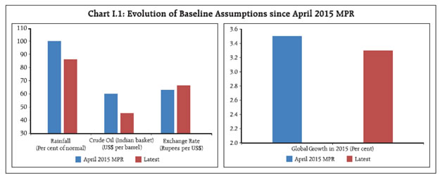

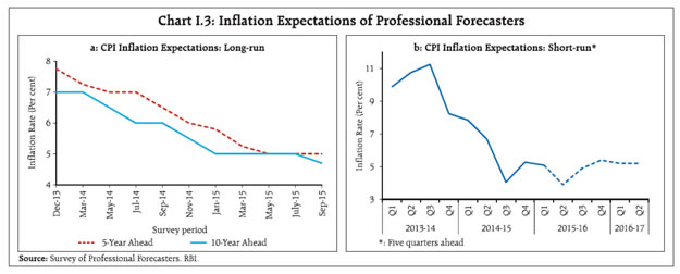

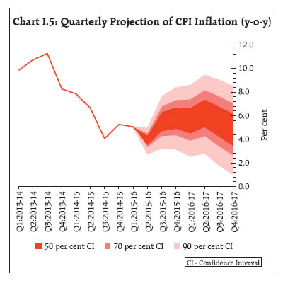
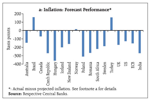

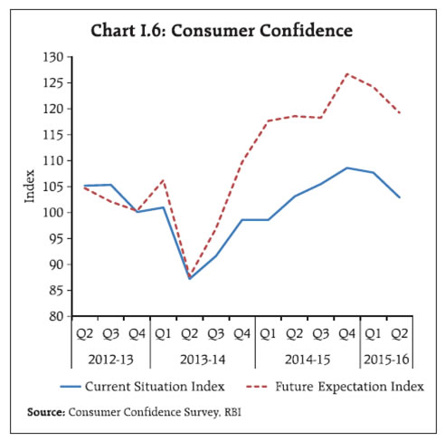
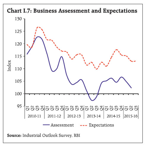

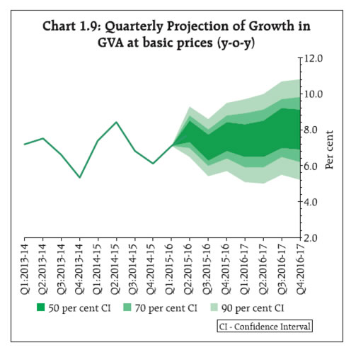
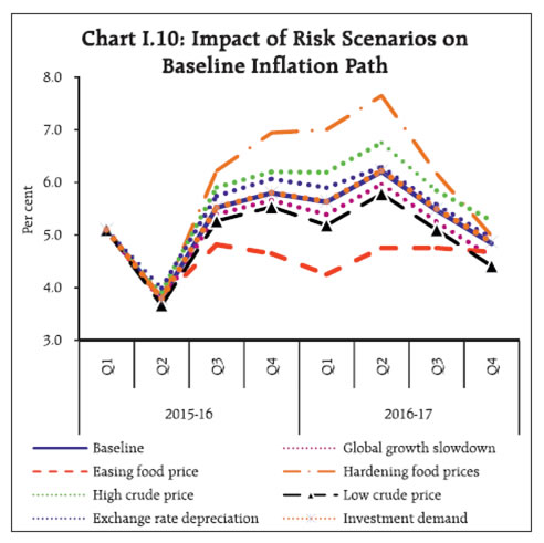

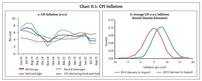
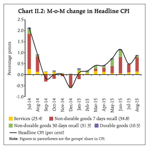

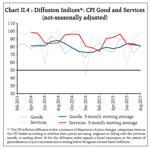
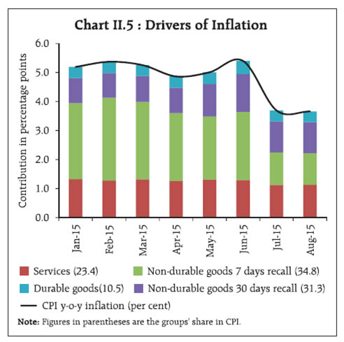

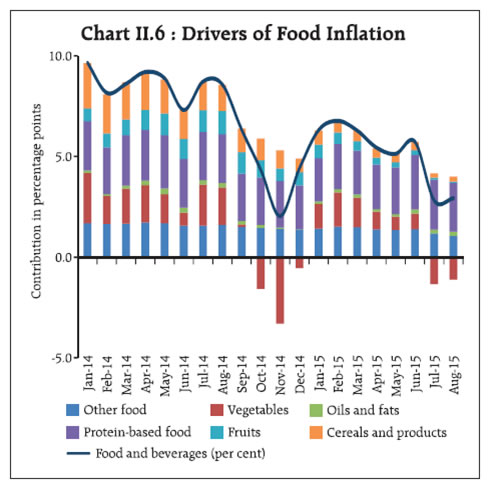

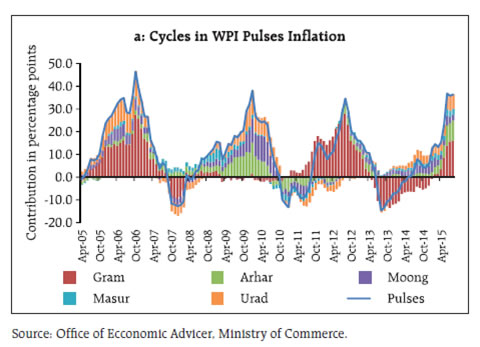
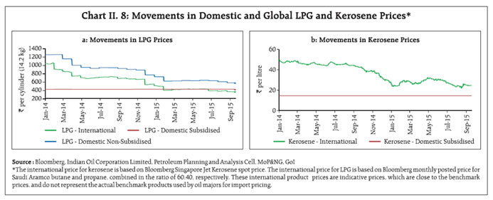

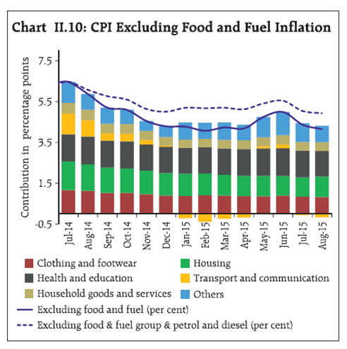

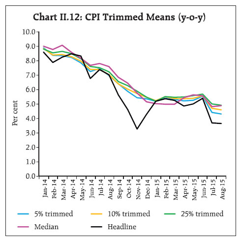
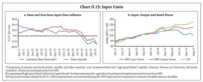
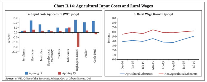
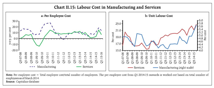

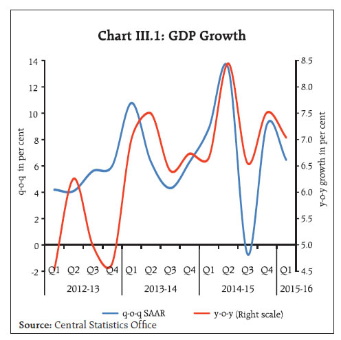

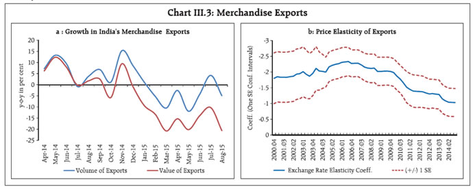

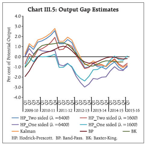


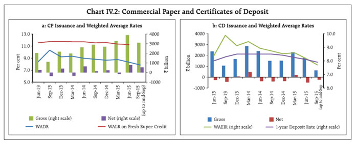


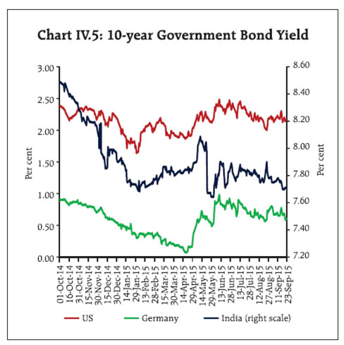

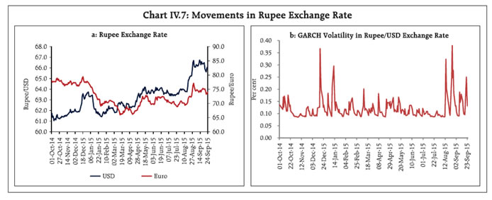
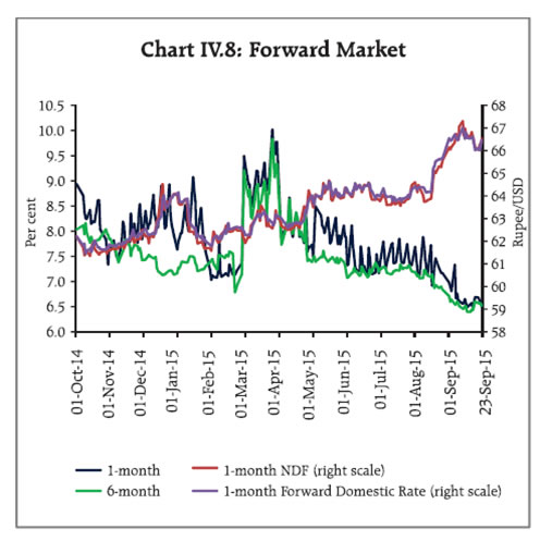


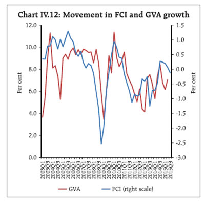
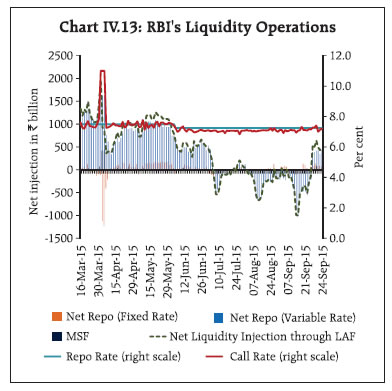
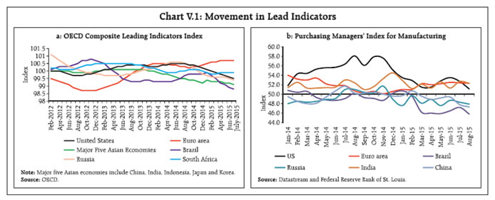

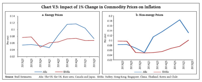
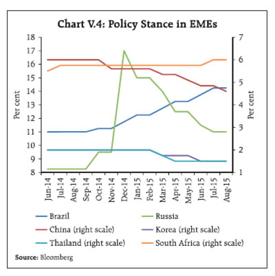

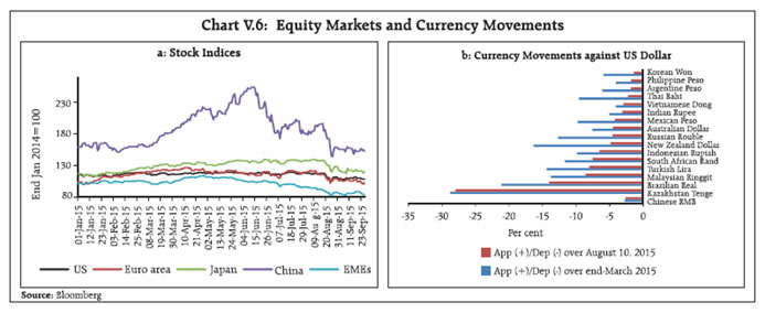
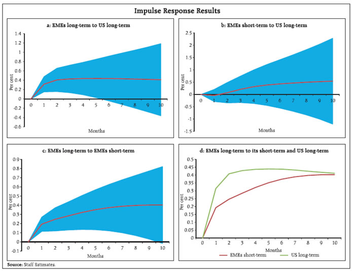

Share this page:


Install the RBI mobile application and get quick access to the latest news!
Scan the QR code to install our app


Page Last Updated on:


