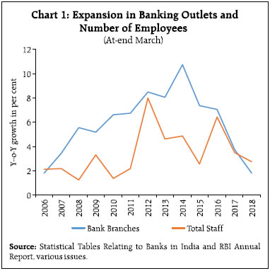
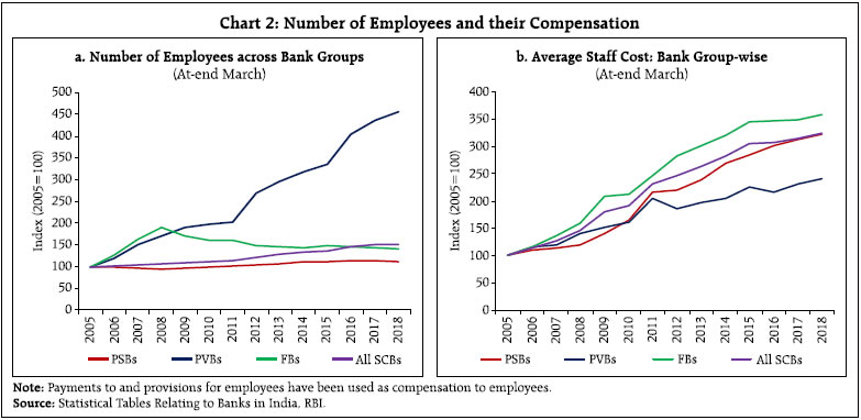
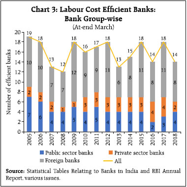
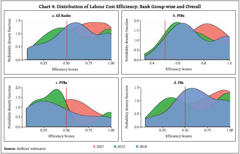
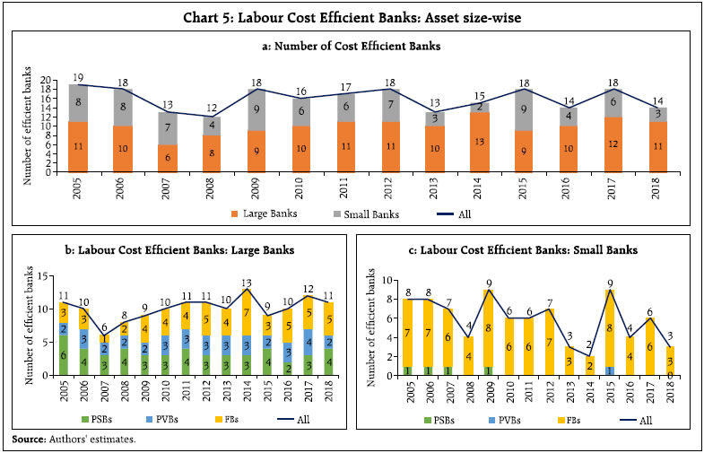
The shift in emphasis from brick-and-mortar operations to digital modes, coupled with increasing per employee output, suggests an improvement in the labour cost efficiency (LCE) of Indian banks. Using Data Envelopment Analysis (DEA) for the period 2005-2018, the results presented in this article show that LCE has not improved. Public sector banks (PSBs) turn out to be more efficient than private sector peers, reflecting deceleration in employment growth as also cost cutting through innovative techniques. Furthermore, large banks are found to be more efficient than small banks as they can reap economies of scale.

Introduction

With 144,952 branches¹ of 159 scheduled commercial banks (SCBs)² catering to the needs of about 1.3 billion people, the Indian banking system is one of the largest in the world. Over the years, its business model has remained primarily brick-and-mortar based although in recent years, the spread of digital modes of transaction has increased significantly. This transformation has become pronounced since 2015 when the number of bank branches began to decelerate. As a corollary, employment growth in the banking sector has also decelerated, which is in line with the international trend (Craig, 1997). Paradoxically, the per employee output of the banking system in terms of deposits, loans and advances, investments and non-interest income has increased during the period, suggesting that labour cost efficiency of the banking system has improved.

The aim of this article is to evaluate this claim empirically. This is a challenging task, since LCE is simultaneously influenced by various factors such as changes in capital, intermediate inputs, technical and organisational changes and economies of scale. Accordingly, non-parametric DEA, which aggregates various input and output indicators into a single measure, is employed in conjunction with the narrative emerging out of the behaviour of key banking aggregates in terms of their labour intensity.

The results of the analysis deviate from the received wisdom: first, notwithstanding increasing use of technology, the LCE of banks in India does not seem to have improved, implying that given labour inputs, Indian banks were not able to optimise output in a period marked by acute risk aversion which is largely exogenous to the labour cost dynamic. Secondly, the results upend the popular belief³ that private sector banks (PVBs) and foreign banks (FBs) are more efficient than public sector banks (PSBs)⁴. In fact, our findings suggest that LCE of PSBs is higher than that of PVBs, mainly reflecting higher per employee output of the former even as staff accretion has decelerated more sharply than in the latter.

The rest of the article is divided into four sections. Section II briefly reviews the literature on efficiency of banks. Section III presents stylised facts and descriptive statistics. In section IV, database, methodology and findings have been discussed. Section V concludes with some policy perspectives.

II. Literature Review

Technical efficiency refers to the ability of a firm to obtain maximum output from a given set of inputs. Allocative efficiency reflects the ability of a firm to use inputs in optimal proportions, given their respective prices. Cost efficiency is the product of the two. It reflects production of output at the minimum cost. Profit efficiency is a comparatively broader concept and takes into account both costs and revenues. It is defined as the ratio of the actual profit of a bank to the maximum level that could be achieved by the most efficient bank (Maudos, et al, 2002).

Recent decades have witnessed a proliferation in analyses of the efficiency of banking and financial institutions focusing on all these aspects and using various methods (Maudos, et al, 2002; Nurboja and Kosak, 2017; Lee and Huang, 2017; Degl’Innocenti, et al, 2017 and Akhigbe, et al, 2017). Among studies on banks in emerging market economies, state-owned commercial banks have been found to be more efficient than the joint-stock commercial banks with an overall improvement in efficiency of Chinese banks during 2003-2011 (Wang, et al, 2014), while smaller banks are found to be less efficient in spite of improvement in efficiency of Brazilian banks during 1998-2010 (Barros and Wanke, 2014).

In India, one strand of the literature focusses on changes in technical efficiency of banks over a period and generally finds an improvement in efficiency after the reforms undertaken in the 1990s (Sensarma, 2006; RBI, 2008; Sarkar and Sensarma 2010; Kumar S. 2013; Bhatia and Mahendru 2015; Badunenko and Kumbhakar 2017). Another strand finds that the efficiency of PSBs improved much more than that of PVBs in the more recent period (Das and Ghosh 2005; Das and Kumbhakar 2010; Kumar, et al, 2016), with State Bank of India and its associates showing the highest efficiency, followed by PVBs and nationalised banks during 2009-2013 (Kaur and Gupta, 2015).

Yet another strand has concentrated on profit efficiency of Indian banks, finding an improvement in profit efficiency over the years, with PSBs being the most efficient relative to their private counterparts (Ray and Das, 2010). Moreover, smaller banks are found to be the least efficient. Profit inefficiency has been traced primarily to allocative inefficiency rather than technical inefficiency during 1999-2012, reflecting the need of optimal utilization of the input-output mix (Jayaraman and Srinivasan, 2014). Efficiency of PVBs reflected more intra-group volatility in relative efficiency changes than PSBs (Kumbhakar and Sarkar, 2003). In contrast, however, improvement in cost efficiency between 1997 and 2003 has been observed (Ray and Das, 2010).

This article focuses on a more narrowly defined concept of cost efficiency viz., labour cost efficiency. On this metric, earlier research found that reforms reduced labour usage during 1985-2003 but inefficiencies existed among large banks, especially Indian PSBs (Jaffry, et al, 2008). Considerable variation in labour cost efficiency was found across branches of a large Indian PSB (Das, Ray and Nag, 2005, Ray, Das and Mukherjee, 2017).

Turning to measurement of productivity/ efficiency, index-based measures such as total factor productivity (TFP) and Malmquist productivity index have been employed as well as DEA, the stochastic frontier approach (SFA) (Coelli, et al, 2005), the Bayesian dynamic frontier model and the Nerlovian profit indicator (Barros and Wanke, 2014; Jayaraman and Srinivasan, 2014). Malmquist productivity index uses distance function approach to measure productivity changes over time. This is also a non-parametric method. On the other hand, stochastic frontier approach is an econometric approach. It uses a pre-specified functional form to estimate inefficiency, modelling it as an additional stochastic term. Further, Bayesian dynamic frontier model uses Bayesian inference in stochastic frontier models by formally incorporating the parameter of uncertainty and by deriving posterior densities of efficiencies for every decision-making unit (DMU). While, the Nerlovian profit efficiency criterion compares the observed profit level with the highest profit level attainable given technology, and output and input prices: an output–input combination is labelled profit efficient if, for given prices, no higher profit level is shown to be attainable.

Ceteris paribus, the DEA has the advantage of flexibility, in that there is no requirement of specifying any functional form of the production process or need for prior assumptions that are inherent in other approaches, such as in econometric approaches to efficiency analysis. Furthermore, it is able to identify performance targets for inefficient units and suggest improvements to achieve Pareto efficiency. It is applicable in cases where the input and output parameters are not clear or uniform, and same efficiency can be achieved using different resource combinations. The freedom to choose multiple inputs and outputs obviates the need to convert all the inputs and associated outputs measures to a uniform unit. It also optimises on weights unlike other techniques where one has to predefine weights of the parameters. It also permits the entities involved to learn from best performing peers and adapt to move towards the efficiency frontier. The DEA is observed to perform well even in case of small number of observations as long as the number of DMUs are sufficiently larger than the number of inputs and outputs (Wong, et al, 2013). Furthermore, it can accommodate multiple inputs and multiple outputs more easily than other methods.

III. Stylised Facts and Ratio Analysis

During the latter half of the 2000s and most part of the 2010s, the growth in bank branches have been much higher than the growth in number of employees (Chart 1).

Labour productivity can be crudely computed by comparing various banking aggregates as output measures per unit of number of employees. Although partial measures of productivity, they are useful in providing quick readings with easy computability.

Although per employee cost of PVBs has grown only moderately, the number of their employees has increased manifold. In contrast, although per employee cost of PSBs has risen more than PVBs, their employee base has remained almost stable. FBs, on the other hand, seem to have employed less but higher paid staff (Chart 2).

An analysis of per employee banking aggregates such as investments, advances, deposits and total income suggests that labour efficiency of PSBs improved over time and they overtook PVBs by 2018 (Table 1). One major reason may be the significant increase in operations carried out by banking correspondents (BCs) on behalf of PSBs. BCs typically earn lower remunerations than bank employees, reducing banks’ input costs. Moreover, the expenditure on BCs is not captured at all in the staff cost account. At the same time, deposits mobilised and credit deployed by the BCs help in pushing up the output indicators of banks. While BCs is a specific example, many other work processes have been outsourced by PSBs in recent years, which may have also led to an increase in labour productivity. On the other hand, a sharper growth in employees seems to have overshadowed the cost advantage of PVBs, leading to moderation in efficiency gains relative to PSBs.

These findings are, however, not unambiguous. For example, when alternate per employee banking aggregates such as non-interest income, operating profit and net profits are used as outputs, the efficiency gains of PSBs are not apparent any more. Therefore, it is necessary to employ a method for aggregating diverse inputs and outputs into a single index to obtain an objective measure of efficiency.

IV. Database, Methodology and Findings

As stated earlier, this paper attempts to analyse the LCE of Indian banks between 2005 and 2018. Labour cost efficiency for these years was computed, although in the interest of brevity, results only for the three years of significance viz., 2007, 2012 and 2018, have been presented: 2007 represents the period just before the onset of global financial crisis, while it was in 2012 that the current banking stress started emerging in India and 2018 is the year for which the latest data is available.

To compute LCE of banks, deposits, loans and advances, investments and non-interest income were taken as outputs whereas number of employees and fixed assets were taken as inputs. Average staff cost and expenses on rent, taxes, lighting, insurance and other administrative costs per unit of fixed assets were taken as input prices for the analysis. All SCBs⁵ were included in the study in order to obtain a comprehensive sample. Thus, the number of banks in our study varies between 75 in 2005 and 84 in 2018⁶. Data have been obtained from various issues of Statistical Tables Related to Banks in India published by the Reserve Bank.

As discussed in Section III earlier, ratio analysis is a partial measure of efficiency as it does not reflect the joint influence of a host of factors such as changes in capital, intermediate inputs, technical and organisational changes and economies of scale. In response to this limitation, we have used DEA, which is a non-parametric linear programming (LP) technique that permits evaluation of the relative efficiency of DMUs without imposing a priori weights on either inputs or outputs. In solving the LP problem simultaneously for a set of DMUs, weights are chosen that maximise the efficiency score of each DMU relative to the best-performing peer or peers. The efficiency of each DMU is measured relative to the efficiency frontier and efficiency scores vary between 0 and 1. If DMU lies on the efficiency frontier, it is labelled as an efficient unit and whichever unit falls below this frontier is referred to as an inefficient unit.

The first fundamental DEA model–named after its developers Charnes, Cooper and Rhodes (DEA-CCR model)–imposes the assumption of constant returns to scale (Charnes, et al, 1978). This assumption would, however, be appropriate only if all the banks in the sample were operating at their optimal scales, which is a very stringent condition. To avoid this condition, the DEA-BCC model–named after Banker, Charnes and Cooper (1984) – extends the DEA-CCR model by allowing variable returns to scale (VRS) (Please see Appendix for details).

For efficiency analysis, SCBs have been divided according to ownership patterns: viz. public, private and foreign banks. Typically, the employee compensation of a bank correlates well with its peers having the same ownership structure but may differ drastically across sectors. Secondly, we have divided the banks on the basis of their asset size into small banks and large banks. It can be hypothesised that larger banks can reap the benefits of returns to scale and may be more efficient; on the other hand, it can be also argued that smaller banks are more agile, can customize their products quickly, thus scoring efficiency gains. Our size-wise analysis will help in deciphering which of the two arguments holds true.

IV.1 Bank group-wise efficiency scores

Input-oriented cost efficiency was used to estimate the efficiency of SCBs for the period 2005-2018. Efficiency scores were computed separately for each year. During 2005, the LCE score of Indian banks was 0.72, which implies that given the input-output bundles, 28 per cent cost could have been reduced while producing the same level of output. In 2018, this score worsened to 0.61. The mean cost efficiencies declined during the period due to the presence of higher technical inefficiencies and moderation in allocative efficiency. This shows that while the banks were relatively efficient in allocating the inputs, they were unable to obtain maximum output from them (Table 2).

The number of efficient banks (banks with a score of 1) varied across the years. Among bank groups, FBs had the largest number of banks on the efficiency frontier. This may be due to their low base in terms of various banking aggregates. Although there was a marked decline in the number of efficient PSBs during 2006-2016, the number of efficient PSBs increased subsequently while that of PVBs declined (Chart 3).

IV.2 Bank group-wise efficiency distributions

Taking a cue from Ray and Das (2010), probability distributions of efficiency scores based on stochastic kernel densities were analysed to gain insights into dynamics of LCE. The efficiency scores across years are not strictly comparable since they are not measured against a common frontier. However, a shift in the skewness of the efficiency frontier may give important insights.

Labour cost efficiency of all SCBs experienced marginal change as the skewness shifted from -0.21 in 2007 to -0.23 in 2018. The probability density function for 2007 was found to be skewed to the left, implying that majority of the banks were lying in the 75-100 per cent efficiency zone. This may be attributed to the robust performance of SCBs in 2007–while deposits and credit accelerated along with an improvement in asset quality, the wage bill decelerated. In 2012, the cost efficiency distribution of all SCBs showed twin peaks with probability of more banks lying within the efficiency range of 30 to 50 per cent than 90 to 100 per cent. This may be a result of the relatively lower order of balance sheet expansion of banks during the year, dip in their profitability and the onset of asset quality woes. Cost efficiency improved in 2018 vis-à-vis 2012 as the probability of number of banks lying in the efficiency range of 50-75 per cent increased. This was probably due to the higher credit off-take by PVBs and FBs as well as the rationalisation of bank branches which led to deceleration in wage bill (Chart 4.a).

PSBs were largely found to be labour efficient as the skewness changed from -0.34 in 2007 to 0.30 in 2018 (Chart 4.b). Throughout the period, a majority of PSBs had efficiency scores greater than 50 per cent. In 2007, the distribution of PSBs was unimodal with a thick right tail, implying the presence of many banks closer to the frontier. This is not surprising since PSBs were performing well then, with low stressed assets. There is a discernible leftward shift in the distribution for 2012, which can be attributed to deceleration in balance sheets and the consequent reduction in their share in total banking assets as well as the deterioration in asset quality which was more pronounced in their case. Many banks lying in the 50-75 per cent efficiency zone in 2012, remained there in 2018 as well, though the distribution reflected twin peaks during the year as the number of banks in the 90-100 percentile increased.

Efficiency distributions of PVBs show marked changes between 2007 and 2012 (Chart 4.c). The distribution was platykurtic in 2007 with a skewness of 0.18. The efficiency of PVBs may have been pulled down by the performance of old PVBs since they witnessed the lowest growth with respect to loans and advances, deposits and investments among all bank groups in 2007. On the other hand, the balance sheet of new PVBs grew in double digits. The distribution became skewed to the right in 2012 with a value of 0.92, signifying an increase in labour inefficiency and the relatively thick left tail in 2012 shows the presence of many inefficient banks below the 50 per cent benchmark. In 2018, however, the skewness of PVBs improved to 0.63 as some banks lying in the low efficiency zone below 50 per cent shifted to higher efficiency zones. The void in the lending space created by PSBs due to mounting non-performing asset (NPA) problems boosted credit supply by PVBs. They also reported higher net profits since their provisioning was relatively lower than PSBs.

In the case of FBs, the majority of efficiency scores were concentrated in above the 50 per cent efficiency zone in 2007 as evident in the skewness value of -0.34. It could be explained by the fact that FBs witnessed significant expansion in balance sheets, supported by acceleration in deposits, loans and advances and investments as well as the highest net profits among all bank groups during the year. The distribution turned bi-modal in 2012 with a skewness value of -0.09. In 2018, their labour efficiency improved as the distribution shifted to the right with a skewness value of -0.24 (Chart 4.d).

IV.3 Bank size-wise efficiency scores

To analyse the efficiency of banks based on their asset size, median values based on asset sizes of banks were calculated for each year, and banks above the median value were considered as large banks while those below it were regarded as small banks.

The number of large banks were 39 and 42 in 2005 and 2018, respectively, while for small banks the numbers corresponded to 37 and 42. In all the years, large banks were found to be more efficient than small banks (Chart 5.a). Among large banks, PSBs initially had most number of banks with efficiency score of 1. After 2009, however, FBs had the largest number of banks on the efficiency frontier (Chart 5.b). In the case of small banks, FBs consistently remained the most efficient bank group throughout the period of study (Chart 5.c). This result is consistent with the results for bank-group wise analysis, which showed that FBs remain the most efficient banks amongst all the bank groups.

IV.4 Bank size-wise efficiency distributions

Large banks tended to be more efficient than small banks as they could reap the benefits of economies of scale. It may also be the case that small banks have limited business operations. The performance of large banks improved marginally as skewness changed from -0.19 in 2007 to -0.33 in 2018. While in 2007, majority of the banks were above the 50 per cent efficiency zone, the probability density plot reflected twin peaks in 2012, with pockets of very efficient banks (efficiency between 90 and 100 per cent) and moderately efficient banks (efficiency between 40 and 60 per cent). The distribution remained bimodal in 2018 as well, with majority of the banks having greater than 50 per cent efficiency (Chart 6).

In the case of small banks, the skewness was 0.11 in 2007, which changed to 0.45 and -0.02 in 2012 and 2018, respectively. In 2012, there was a noticeable shift in skewness of small banks to the right, indicating that the concentration of bank efficiency moved away from the frontier. However, there was a recovery in 2018. Among them, foreign banks were mostly found to be lying on the frontier. It may be noted that the small banks group is dominated by foreign banks.

V. Conclusion

Our findings show that during the period 2005-2018 the labour cost efficiency of Indian banks moderated across all bank groups. The deterioration was especially marked during 2011-2016–a period that was characterized by severe stress in the banking sector– an exogenous factor not controlled by the labour cost dynamic. Second, our analysis suggests that PSBs scored relatively better than other bank groups. This has important policy implications as it demonstrates that labour cost efficiencies can be augmented by rationalising work processes. This opens up the avenue of rationalisation in work flow by harnessing new technologies. In this context, payments banks, which are expected to leverage technology, could offer a laboratory experiment and it would be interesting to study their labour cost efficiency once data becomes available.

Finally, our results point to larger banks being labour cost efficient relative to their smaller counterparts as the former can reap the benefits of economies of scale. This finding provides an additional rationale for recent mergers of banks, both amongst PSBs and PVBs and suggests that further avenues of consolidation in the banking sphere may be explored.

References

Akhigbe, A., McNulty, J.E., and B.A. Stevenson (2017), “Does the form of ownership affect firm performance? Evidence from US bank profit efficiency before and during the financial crisis”, The Quarterly Review of Economics and Finance, 64:120-129.

Badunenko, O. and S.C. Kumbhakar (2017), “Economies of scale, technical change and persistent and time-varying cost efficiency in Indian banking: Do ownership, regulation and heterogeneity matter?”, European Journal of Operational Research, 260(2): 789-803.

Banker, R. D., Charnes, A. and W. W. Cooper (1984), “Some models for estimating technical and scale inefficiencies in Data Envelopment Analysis”, Management Science, 30(9): 1078-1092.

Barros, C.P. and P. Wanke (2014), “Banking efficiency in Brazil”, Journal of International Financial Markets Institutions and Money, 28(1): 54-65.

Bhatia, A. and M. Mahendru (2015), “Assessment of Technical Efficiency of Public Sector Banks in India Using Data Envelopment Analysis”, Eurasian Journal of Business and Economics, 8(15): 115-140.

Charnes, A., Cooper, W.W. and E. Rhodes (1978), “Measuring the efficiency of decision making unit”, European Journal of Operational Research, 2: 429-444.

Coelli, T. J., Rao, D., O’Donnell, C.J. and G.E. Battese (2005), An Introduction to Efficiency and Productivity Analysis, New York: Springer.

Craig, Ben R. (1997), “The Long-run Demand for Labor in the Banking Industry”, Federal Reserve Bank of Cleveland, Economic Review, 33: 23-33.

Das, A. and S.C. Kumbhakar (2010), “Productivity and Efficiency Dynamics in Indian Banking: An input distance function approach incorporating quality of inputs and outputs”, Journal of Applied Econometrics, 27: 205-234.

Das, A. and S.Ghosh (2005), “Financial Deregulations and Efficiency: An empirical analysis of Indian Banks during the post reform period”, Review of Financial Economics: 193-221.

Das, A., Ray, S. and A.Nag (2005), “Labor-Use Efficiency in Indian Banking: A Branch Level Analysis”, Economics Working Papers. 200504, University of Connecticut.

Degl’Innocenti, M., Kourtzidis, S.A., Sevic, S. and N.G. Tzeremes (2017), “Bank productivity growth and convergence in the European Union during the financial crisis”, Journal of Banking & Finance, 75: 184-199.

Jaffry, S., Ghulama, Y. and J. Cox (2008), “Labour use efficiency in the Indian and Pakistani commercial banks”, Journal of Asian Economics:259–293.

Jayaraman, A.R. and M.R. Srinivasan (2014), “Analyzing profit efficiency of banks in India with undesirable output - Nerlovian profit indicator approach”, IIMB Management Review, 26(4): 222-233.

Kaur, S. and P.K. Gupta (2015), “Productive Efficiency Mapping of the Indian Banking System Using Data Envelopment Analysis”, Procedia Economics and Finance, 25: 227-238.

Kumar, M., Charles, V. and C.S. Mishra (2016), “Evaluating the performance of Indian Banking sector using DEA during post-reform and global financial crisis”, Journal of Business Economics and Management, 17(1): 156-172.

Kumar, S. and M.Sreeramulu (2007) “Employees’ Productivity and Cost – A Comparative Study of Banks in India During 1997-2008”, Reserve Bank of India Occasional Papers, Winter.

Kumar, Sujeesh (2013), “Total Factor Productivity of Indian Banking Sector - Impact of Information Technology”, Reserve Bank of India Occasional Papers, 34 (I & II): 66-85.

Kumbhakar, S.C. and S.Sarkar (2003), “Deregulation, Ownership and Efficiency in Indian Banking”, Arthaniti-Journal of Economic Theory and Practice, 2(1-2): 1-26.

Lee, C. and T. Huang (2017), “Cost Efficiency and Technological Gap in Western European Banks: A Stochastic Metafrontier Analysis”, International Review of Economics and Finance, 48: 161-178.

Maudos, J., Pastor, J.M., Francisco, P. and Q. Javier (2002): “Cost and profit efficiency in European Banks”, Journal of International Financial Markets, Institutions and Money,12: 33–58.

Nurboja, B. and M. Košak (2017), “Banking efficiency in South East Europe: Evidence for financial crises and the gap between new EU members and candidate countries”, Economic Systems, 41(1): 122-138.

Ray, S. and A. Das (2010), “Distribution of cost and profit efficiency: Evidence from Indian Banking”, European Journal of Operational Research: 297–307.

Ray, S.C., Das, A. and K. Mukherjee (2017), “Labor-Cost Efficiency with Indivisible Outputs and Inputs: A Study of Indian Bank Branches”, Working papers 2017-04, University of Connecticut, Department of Economics.

Reserve Bank of India (2008), “Efficiency, Productivity and Soundness of the Banking Sector.” Reports on Currency and Finance - Special Edition, Chapter IX.

Sarkar, S. and R. Sensarma (2010), “Partial Privatization and Bank Performance: Evidence from India”, Journal of Financial Economic Policy, 2: 276-206.

Sensarma, Rudra (2006), “Are foreign banks always the best? Comparison of state-owned, private and foreign banks in India”, Economic Modelling, 23: 717–735.

Wong, P.Y.L., Leung, S.C.H. and Gilleard, J.D. (2013), “Facility Management Benchmarking: An Application Of Data Envelopment Analysis In Hong Kong”, Asia-Pacific Journal Of Operational Research, 30 (5).

Wang, K., Huang, W., Wu, J. and Y.N. Liu (2014), “Efficiency Measures of the Chinese Commercial Banking System Using an Additive Two-Stage DEA”, Omega, 44: 5-20.

Appendix

Estimation of Labour Cost Efficiency through DEA

Following Coelli. T.J (1996), let us consider DEA-CCR model with K inputs and M outputs for each of N DMUs. Vectors xi and yi represent inputs and outputs, respectively for the i-th DMU. The KxN input matrix, X, and the MxN output matrix, Y, represent the data of all N DMUs. As alluded to earlier, DEA constructs a non-parametric envelopment frontier such that all points lie on or below the production frontier.

For each DMU, ratio of all outputs over inputs u’y_i/ v’x_i is computed where u is Mx1 vector of output weights and v is a Kx1 vector. Optimal weights are calculated by: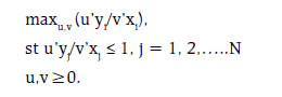

This results in finding values for u and v such that efficiency measure of the i-th DMU is maximised subject to the constraint that all efficiency measures must be less than or equal to one. However, this leads to an infinite number of solutions which can be overcome by imposing the constraint v’x_i =1 so that, u and v change to μ and ν shows the transformation.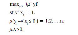

Using the duality in linear programming, the following envelopment form can be derived: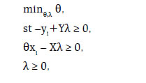

where θ is a scalar and λ is a Nx1 vector of constants. The value of θ is the efficiency score of the i-th DMU such that θ≤1 with a value of 1 indicating an efficient DMU lying on the frontier. The linear programming problem is solved N times, for each DMU, to obtain a value of θ for each.

The CRS assumption would only be appropriate if all banks in the sample were operating at their optimal scales, which is a very stringent condition and will also lead to faulty results due to the inclusion of scale inefficiencies. To avoid this condition, the DEA-BCC model named after Banker, Charnes and Cooper (1984) extends the DEA-CCR model by allowing variable returns to scale (VRS).

Since CRS model is valid only if all units in the sample are operating at their optimal scale, the CRS linear programming is modified to account for VRS adding the convexity constraint N1’ λ=1 to the above equation: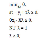

where N1 is an Nx1 vector of ones. This approach forms a convex hull of the observed input-output bundles.

For cost minimisation, the following DEA is run: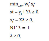

where w_i is a vector of input prices for the i-th DMU and x_i* is the cost-minimising vector of input quantities for the i-th DMU given the input prices w_i and the output levels y_i. The total cost efficiency (CE) of the i-th DMU will be calculated as

The cost efficiency (CE) of the i-th bank is the ratio of the minimum cost to the actual cost or observed cost.

However, here all inputs are assumed to be variable and hence, firms can vary the inputs to achieve efficiency. Therefore, efficiency measure has to be modified to include quasi-fixed inputs. Following Das, et al. (2005), we assume input vector x_i can be partitioned as x_i= {α_i, Q_i} where α_i is the vector of variable inputs while Q_i is the vector of quasi-fixed inputs. The input price vectors are r_i and p_i for variable and fixed inputs, respectively. Since fixed cost is constant in the short run, it plays no role in cost minimisation in the short run. Therefore, we compute efficiency through variable cost minimisation. The minimum variable cost of the firm is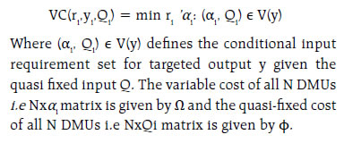

The DEA model for variable cost minimisation is: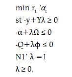

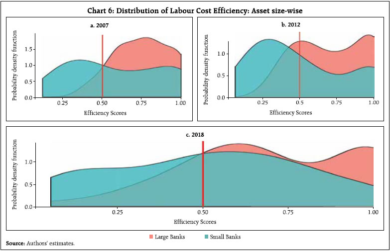
The variable cost efficiency of the i-th firm is given by

where α_i* is the vector of cost minimising variable input for the i-th DMU.

* This article is prepared by Snehal S. Herwadkar, K. M. Neelima, Radheshyam Verma and Preeti Asthana (Research Intern), Department of Economic and Policy Research. The views expressed in the article are those of the authors and do not represent the views of the Reserve Bank of India.

¹ At end-September 2018.

² Including regional rural banks, small finance banks and payments banks.

³ For example see https://www.karvy.com/who-gives-the-best-deal-psu-or-private-banks; downloaded on February 8, 2019.

⁴ Kumar and Sreeramulu (2007) found that the performance of private sector banks (PVBs) and foreign banks (FBs) in terms of labour productivity was superior to public sector banks (PSBs) during 1997-2008 using exploratory data analysis.

⁵ Excluding regional rural banks, payments banks and small finance banks.

⁶ The number of banks varies as many new FBs started functioning during the period, while the number of PVBs changed due to various mergers and acquisitions and licensing of new banks. Further, various associate banks of State Bank of India (SBI) got merged with SBI during this period.