 IST,
IST,


RBI WPS (DEPR): 02/2015: Public Debt Management in India and Related Issues
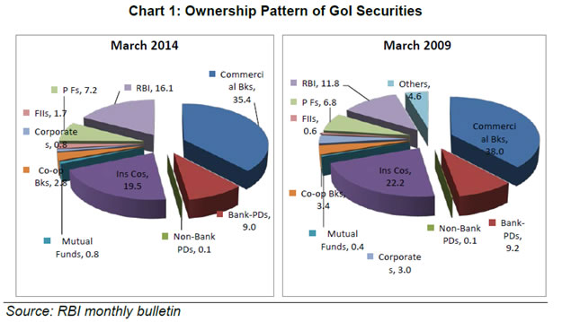
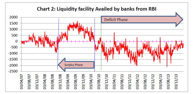
| RBI Working Paper Series No. 02 Abstract *The public debt management in India has clearly traversed from a passive system to a market driven process with developed institutions, instruments, widespread investors, intermediaries for market making and efficient market infrastructure. Towards the PDM objective of minimising the cost of borrowing over the medium to longer term, market factors, both long and short term, affect the bond yield. Though the borrowings of the Government is sovereign and its long term yield is generally determined by expected liquidity risk, repayment risk, economic prosperity and the inflation expectations, sudden shocks in short term factors like availability of liquidity (fund) and the cost of such liquidity play a major role on the yield. Impulsive response function under unrestricted VAR framework confirms that when a policy action is taken to increase the system liquidity, the bond yield declines immediately and thereafter, the yield stabilizes at a level lower than the level before the shock was effected. It may be more evident that a shock to the repo rate has positively impacted the yield of securities with all maturities up to 30 years. Further, expectation of increase in repo rate has significant and immediate impact on the yield. Overall, the study supports the arguments that the system liquidity and the cost of funds are also factors that influence the yield of the G-Secs in the primary market. JEL Classification: H630: Debt; Debt Management; Sovereign Debt Keywords: Debt, Government Bonds, Treasury, Treasury Securities Introduction Sovereign Debt Management (SDM) is the process of establishing and executing a strategy for managing the government's debt in order to raise the required amount of funding, achieve its risk and cost objectives and to meet any other sovereign debt management goals the government may have set, such as developing and maintaining an efficient market for government securities (IMF 2001). The importance of public debt management (PDM) as part of public policy is to ensure that both the level and rate of growth in public debt is fundamentally sustainable in a broader macroeconomic framework. In this context, debt structures and strategies including prudent risk management are crucial as the macroeconomic consequences of sovereign debt default on the economy can be severe. The consequences, among others, include weakening long term credibility and capability of the government to mobilize resources as also increase in cost. The largest financial portfolio in a country is the government's debt portfolio, which can generate substantial risk to the balance sheet of the government and the financial stability of the country. At the basic level, sovereign debt management addresses the structure and composition of the public debt portfolio, including the desired mix in terms of currency, interest rate and maturity profile (Ian Storkey, 2001). Therefore, it is essential that sound risk management along with country specific public debt structures are to be put in place to reduce government’s exposure to market risk, rollover risk, liquidity risk, credit risk, settlement risk and operational risk. Recent financial crises have highlighted the importance of sound debt and risk management practices as also sound fiscal and monetary coordination and management. In India, sovereign debt is largely domestic and within that marketable debt is the largest component, which is managed by the Reserve Bank of India (RBI). Since recently, market borrowing has been the largest financing item of fiscal deficit for the Central and State Governments. Accordingly, this study focuses on the marketable domestic public debt of the Government of India (GoI) in terms of size, magnitude, policy and approach followed and also discusses issues and challenges on debt management. Though various factors decide the yield in the primary auction, which include the growth in the economy, market conditions, ruling interest rate, long term perspective on the inflation expectations, etc., in a deficit liquidity scenario, the main determinants may be the ruling short term interest rate (repo, MSF) that determines the cost of fund and the availability of market liquidity. Thus, how far these short term factors influence the yield in the primary auctions is the focus of this paper. Against the above background, a brief evolution of PDM in India is attempted in Section 1. International experience of the SDM is briefly discussed in Section 2. In this section, the guidelines issued by the IMF-World Bank have been compared with Indian conditions. The present debt management policy/practices of GoI along with the issues and challenges are set out in Section 3. In Section 4, an attempt has been made to test the impact of the availability of system liquidity and its cost on the primary yield of G-Secs through an unrestricted VAR framework, supported by two mean t-test. Concluding observations and policy options are drawn in Section 5. 1. Evolution of Public Debt Management in India The main objective of PDM in India, in particular, management of market borrowings, is to minimise the cost of borrowing over the medium to longer term as also to contain the rollover risks while raising the borrowings of the Governments. Since its incorporation, the RBI took over the responsibility of managing the public debt of the Centre and the sub-nationals, besides playing the role as a banker in an environment when the financial system was underdeveloped. Prior to the reform period, debt management in India was characterised by issuance of debt at administered interest rates to a captive investors, i.e., banks and financial institutions. Among the reform process initiated, the first initiative was to allow market determined rates in the primary issuance for government securities through auctions in 1992. Second, the market infrastructure was to be developed to take care of auctioning, secondary market trading, payment and settlement system. Third, benchmark was to be developed for fixed income instruments for the purposes of their pricing and valuation. Fourth, an active secondary market for G-Secs was also needed to increase the liquidity as also for operating monetary policy through indirect instruments such as open market operations and repos to manage short-term liquidity. Reforms, therefore, focused on the development of appropriate market infrastructure, elongation of maturity profile, increasing the width and depth of the market, improving risk management practices and increasing transparency (Mohan 2008). Since 1991-92, strengthening the quality of government debt management was a key element of the policy reform packages. Two landmark developments have shaped India’s PDM framework, viz., (i) supplemental agreement between the RBI and the GoI in March 1997 and (ii) Fiscal Responsibility and Budget Management (FRBM) Act1 in 2003. The issuance of ad-hoc treasury bills by the GoI to the RBI to finance the fiscal deficit was discontinued with the supplemental agreement and with the FRBM Act, the RBI has been prohibited from participating in the primary auctions of government securities. Thus, with the above two developments, monetization of fiscal deficit is not allowed. For smooth transition to the new system, the RBI has taken a number of measures to make the G-Sec market deeper, broader and more liquid while improving trading, settlement, intermediaries, institutional and infrastructure development. Towards this direction, reforms in the G-Sec market were aimed at enhancing liquidity and efficiency, which include establishment of Delivery versus Payment system (DvP) to reduce settlement risk, institution of Primary Dealer (PD) system to act as market makers, and formation of market bodies. Instrument diversification was also seriously attempted during this phase of reforms. Further reform measures include (a) operationalisation of the Negotiated Dealing System (NDS), an automated electronic trading platform; (b) establishment of Clearing Corporation of India Limited (CCIL) for providing an efficient and guaranteed settlement platform; (c) introduction of trading of G-Secs in stock exchanges; (d) introduction of OTC and exchange-traded derivatives to facilitate hedging of interest rate risk; (e) introduction of Real Time Gross Settlement System (RTGS), which addresses settlement risk and facilitates liquidity management; (f) adoption of a modified DvP mode of settlement (DvP III), which provides net settlement of both funds and securities legs; and (g) announcement of an indicative auction calendar for Treasury Bills (TBs) and dated securities (RBI, 2007). In order to boost the market liquidity and to provide hedging facility, various derivatives and other products have been introduced in the G-Sec market. The NDS auction platform replaced with a wider spectrum of e-kuber module in the core banking solution platform in October 2012, which also acts as anytime and anywhere banking. The process of Government debt management mainly encompasses establishing clear debt management objectives and supporting them with a sound governance framework, prudent debt management strategy and reporting procedures to ensure that the government’s debt managers are accountable for implementing the debt management responsibilities delegated to them (World Bank 2014)2. Further, for domestic debt management, debt managers have adopted practices aimed at reinforcing the government’s reputation as a predictable and consistent issuer, committed to promoting competition among investors and ensuring a high degree of transparency regarding its decision making. At micro level, debt managers issue securities in a range of maturities in order to diversify their refinancing risk, committed to principles of transparency by publishing borrowing calendar well in advance and removing regulatory distortions that discriminate among investors. Capacity building needs in PDM are country specific. Countries in the nascent stage of development of G-Sec market preferred to issue simple and standard instruments and a mix of conventional and complex instruments are being introduced over the years when the bond market develops. The recent financial crisis highlighted the importance of containing risks in debt management. While developing debt management strategies, debt managers are often required to manage different types of risks (Box 1).The risks inherent to the government debt structure are monitored and a range of policies are engaged to manage these risks with trade-offs between costs against risks. Box 1: Risks Associated with Sovereign Debt Management3 Market Risk: Market risk is associated with changes in market conditions such as interest rate, exchange rate, commodity prices, and the concomitant impact on the cost of debt servicing of the Government. Changes in interest rates affect debt servicing costs, when fixed rate debt is refinanced and the coupon of floating rate debt is reset. Hence short term debt is usually considered to be more risky than long term fixed rate debt. Therefore, the RBI issues a combination of both fixed and floating rate securities, but mainly strategies for fixed rate securities, with maturities upto 30 years. Refinance Risk/ Rollover Risk: In a changing interest rate scenario, the debt is to be rolled over at an unusually high cost or, in extreme cases, cannot be rolled over at all is a risk. Relatively high average maturity of debt would result in a lower share of debt rollover in a year. In India, the average maturity of the securities outstanding is around 10 years and buyback/switch operations have been effected in addition to elongation of maturity to contain the rollover risk. Liquidity Risk: Liquidity risk is considered to be two types. The first one refers to the cost the investors face in trying to exit a position when the number of transactors has markedly decreased or because of the lack of depth of a particular market (IMF-World Bank, 2001). The second one refers to a situation in which the volume of liquid assets diminishes quickly in the face of unanticipated cash flow obligations or a possible difficulty in raising the borrowings in a short period of time. In India, the RBI has been reissuing GoI dated securities to build critical mass and impart liquidity in the secondary market. While liquidity is limited to a few securities, all G-Secs are acceptable as collateral at the LAF window of the RBI for availing liquidity facility. Credit Risk: Credit risk is particularly relevant in cases where debt management includes the management of liquid assets. It may also be relevant in the acceptance of bids in auctions of securities issued by the government as well as in relation to contingent liabilities and derivative contracts entered into by the debt manager (IMF-World Bank, 2014). In India, the Clearing Corporation of India Limited (CCIL) acts as the central counter party (CCP) framework that eliminates counterparty credit riskSettlement Risk: Refers to the potential loss that the government could suffer as a result of failure to settle, for whatever reason other than default, by the counterparty. In India, the CCIL has been assigned the role of CCP by novation and the settlement is taking place in the form of delivery vs payments (DvP) thereby the settlement risk is mitigated. Operational Risk: Different types of operational risks such as transaction errors in the various stages of executing and recording transactions; inadequacies or failures in internal controls, or in systems and services; reputation risk; legal risk; security breaches; or natural disasters that affect business activity (IMF-World Bank, 2001). In India, the well laid down operational procedures with inbuilt internal control, segregation of duties with front office, middle office and back office structures coupled with latest technology with inbuilt controls in primary and secondary market operations contain operational risks. A major feature of government financing in developing countries is the reliance on captive sources of funding, whereby financial institutions are required to purchase and hold government securities, often at below market interest rates, or administered interest rates, which is diminishing in many countries. The negative impact of reliance on captive sources of funding is that it stifles the development of G-Sec markets and thereby affects the secondary market trading and liquidity. While the removal of such captive investor base may have increased interest rates to market determined levels in the short run, the ensuing deep and liquid government securities market in the medium to long term is expected to reduce the debt service costs for the governments in future (IMF-World Bank, 2002). In the literature, studies have attempted to assess the impact of fiscal shocks on the sovereign yield curve. There is a common trend in yield differentials, which is correlated with a measure of aggregate risk. In contrast, liquidity differentials display sizeable heterogeneity and no common factor. Carlo Favero et al (2008) observed that the yield differentials should increase in both liquidity and risk, with an interaction term of the opposite sign. A sound debt management strategy is the efficacy of tactical liability management operations, in which debt managers credibly intervene in domestic debt markets in emergency situations and quickly rebuild investor confidence. The low level of market development in most developing countries, the still vulnerable structures of debt in many emerging market economies and the rise in debt levels in a number of developed economies make sound sovereign debt management even more challenging for global financial stability in the future, particularly given the higher global funding pressures (IMF 2010). The liquidity effect emanating from various macroeconomic shocks would have a distinct impact on yields although expectations on economic advancements also play an important role. The SDM has come in the forefront after the recent global financial crisis as debt surged to unsustainable levels in many advanced countries, triggering sovereign debt crises in countries like Greece, etc. International experience reveals that, prudent debt management can reduce financial volatility by spreading maturity, avoiding captive funding by target investors and developing widespread investors’ base. Another takeaway for PDM is to issue diversified instruments with innovative secondary market products to broaden and deepen the securities market. Transparency in information disclosure and good governance can instill confidence in investors and encourage efficient pricing. 3. Public Debt Management in India - Issues and Challenges As envisaged in the guidelines by the IMF-World Bank, a consensus is evolving world over in which the main objective of PDM is to ensure that the government’s financing needs and its payment obligations are met at the lowest possible cost over the medium to long run, consistent with a prudent degree of risk, which would be smoothened by development of an efficient and liquid government securities market. In its endeavor as a debt manager, the RBI has adopted similar objectives of minimizing the cost of borrowings for the Government, maintain acceptable rollover risk, develop deep and liquid bond market and widen the investors’ base. Keeping in view the various issues and challenges that confront the debt management structure, this study attempts to assess the policies and procedures to minimize the risks in achieving the objectives of debt management. In the light of the different types of risks in debt management operation (Box 1 of the previous Section), the process of debt management strategy is studied through stylized facts such as approaches adopted, maturity profile, timing of issue, costs, different debt instruments and other competing requirements, which are country specific. Some of the issues and challenges that confront the debt management in the Indian context are as under. 3.1 Managing the large size of borrowing Market borrowings have been the discretionary part in government’s total borrowing programme in recent period and have emerged as the dominant source of financing of fiscal deficit, which has increased from around 18 per cent in 1990-91 to 86 per cent in 2007-08 and, thereafter to 93 per cent in 2011-12. The gross market borrowings of the GoI and States together has more than doubled in the current decade as compared with the beginning of the previous decade (1999-00) (Table 1). It is a challenge to mobilize such a huge market borrowings as well as meet the objective of minimizing the cost to Government. As higher market borrowings lead to enhanced supply of government securities, which demand higher yield leading to higher benchmark rate. Further, this would feed in to inflation through input costs and push up benchmark and thereby creating a vicious cycle. Hence, this trend would pose challenge for the debt manager in devising a strategy so that benchmark does not come under pressure and remains market aligned. It may also increase the spread between the GoI and comparable securities and would pose a risk for smooth and orderly conduct of debt management operations and also a challenge to the basic objective of borrowings at a lower cost in the medium to long run. 3.2 Sustainable Public Debt As part of public policy, debt management framework also ensures that the impact of government financing requirements and debt levels on borrowing costs are sustainable. The sustainability of debt requires governments to be both solvent and liquid, i.e., a country’s ability to service all accumulated government debt at any point in time. Generally, the issue of debt sustainability is analysed through ratios such as debt service ratio, interest payments to net tax revenue, debt to exports and public debt to GDP among others. Cross-country analysis and simulations suggest that a debt to GDP ratio in the range of 60-65 percent by 2015/16 might be suitable for India (IMF, 2010). Debt is said to be tolerable if its servicing does not impose an intolerable burden on the fiscal position. Interest payments as one-fifth of revenue receipts are considered a tolerable ratio of interest burden (Dholakia et al, 2004). In India, debt service payments (repayment + interest payment) to revenue receipts has declined to around 37 per cent in 2011-12 from 51 per cent in 1999-00 indicating higher revenue resource mobilization by the GoI as also reign on growth in public debt. Interest payments to net tax revenue declined from 56.5 per cent in 2004-05 to 41.1 per cent in 2010-11. Similarly, interest payments to revenue receipts also declined during the period. In India, the debt to GDP ratio has been steadily declining which is an indication that India's public debt is sustainable. While the public debt of the Centre has increased marginally from 39.4 per cent to 40.5 per cent during 2006-07 to 2012-13, the states position has been declining from 21.2 per cent to 15.9 per cent during the period. The combined public debt to GDP ratio (GoI + States) stood well within the standard level prescribed by the IMF for EMEs at 63–78 per cent. Reflecting these trends, the total liabilities of the general Governments has declined from about 73 per cent in 2006-07 to 65.3 per cent in 2013-14 (Table 2). 3.3 Improve the Resilience of Debt Structure and Strategy The appropriate debt strategy depends upon the government’s tolerance limits to various risks. For which, the strategic portfolio benchmarks is usually supported by a risk management framework that ensures the risks are well specified and managed, and that the overall risk of debt portfolios is within acceptable tolerances (World Bank 2005). To improve the resilience of the debt structure, liability management operations to elongate the maturity and thereby reduce rollover and liquidity risk are attempted by debt managers. In India, as part of prudent debt management strategy, the RBI has elongated the maturity profile of the outstanding stock of G-Secs by issuing securities of longer maturity in order to minimize the rollover risk and by capping the debt repayment in a particular year. Further, the short term debt is very meager and constitutes a very small portion of total debt. As a result, the weighted average maturity of primary issuances of the GoI dated securities increased from 9.4 years in 2001-02 to 13.5 years in 2012-13. The weighted average maturity of outstanding stock of government securities declined from 10.59 years in 2007-08 to 9.7 year in 2012-13, which, however, increased to 10 years in 2013-14. In India, the well laid down operational procedures coupled with the latest technology in primary and secondary market operations with inbuilt internal control limits contain operational risks, which continues to be minimized through several measures. These internal control measures, implemented in line with international best practices and risk management principles, include segregation of duties, dual access control for auction systems, separate payment and settlement mechanism, etc. With the effective debt management strategies of the RBI, the cost of borrowings of the GoI dated securities has declined from 14.3 per cent in 2001-02 to 8.5 per cent in 2011-12 and further to 8.36 per cent in 2012-13. Similarly, the weighted average cost of the outstanding stock of GoI securities also declined from 9.3 per cent in 2003-04 to 7.98 per cent in 2013-14 (Table 3). In the case of sub-national borrowings, the weighted average yield has increased gradually from 8.79 per cent in 2011-12 to 9.18 per cent in 2013-14, which however declined substantially to 8.58 per cent in 2014-15. 3.4 Demand Side Risk and Promoting Retail Segment for Government Securities Demand side risk generally referred to sudden shifts in the demand for government bonds due to interest rate variations. Demand side risk could be addressed through spreading the issuance of securities along the yield curve during the year, which would increase the attractiveness to investors and reduce the liquidity premium that investors demand. This would also reduce the risk that the pricing of government securities are usually affected by the actions of a small number of captive market participants (IMF-World Bank, 2001). The Indian debt market remains largely a wholesale market dominated by banks, financial institutions and insurance companies; there has been entry of cooperative banks, RRBs, mutual funds and non-banking financial companies (NBFCs) in the recent period. Additionally, the entry of 100 per cent gilt mutual funds has broadened the retail investors’ base. The holding pattern of G-Secs reveals that banks including bank-PDs hold about 44 per cent of G-Secs followed by insurance companies at 20 per cent as at end-March 2014. Investment by pension funds constitutes about 7 per cent (Chart 1). Reliance by governments on captive sources of funding whereby financial institutions are required to purchase G-Secs is diminishing in many countries. In India, though the reserve requirements by the scheduled commercial banks have come down significantly from 38 per cent of their demand and time liabilities in 1990 to 22 per cent by August 2014, still it is considered to be high. In the eventuality of a decline in reserve requirements, alternative set of investors, particularly retail investors, to fund the government borrowings needs to be put in place well in advance. Gradual move to reduce the upper limit on held-to-maturity (HTM) category of G-Sec holdings by banks has been initiated so as to stimulate the secondary market trade and thereby increase the liquidity of the G-Secs. Catering to the needs of retail investors will contribute to a stable demand for G-Secs, which can cushion the impact of sales from financial institutions and FIIs at times of volatility. However, retail participation in the Indian G-sec market is limited. Mid-segment investors such as cooperative banks, pension funds, etc., are also limited in G-Sec investments in India. A web-based NDS-OM module has been in place since June 2012, enabling retail investors to transact in G-Secs in the secondary market and details on these modules have been placed on RBI web-site. As government debt in India is solely in domestic currency and being sovereign, i.e., risk-free retail investor need to be targeted as they hold the securities till maturity thus add stability to the holding pattern of G-Secs. As suggested by a Working Group (RBI, 2012), utilizing the services of banks and Post Offices as a distribution channels and nodal point for interface with individual investors could be examined. Though, the RBI has been conducting regional workshops and seminars for the mid-segment investors like UCBs, RRBs, etc., further investors’ education would go a long way in improving the retail participation. In this context, PDs also need to make a greater effort to promote the mid-segment investors. Finally, though the FII limits in the G-Sec market have been increased in a calibrated manner, however, they had earlier approached the secondary market through brokered trades, which transformed into custodian approach. However, direct access to G-Sec market by the FIIs would pose their dominance in the market, which may lead to rigging the market and thereby more volatility like the equity market. Thus a fine balance needs to be worked out.3.5 Benchmarking and Consolidation To manage the associated rollover risks, Government used to often buildup liquid financial assets in benchmark issues, spread the maturity profile of the debt portfolio across the yield curve, and use domestic debt buybacks, conversions or switches of older issues with new issues. Liquid debt market is important for development of a healthy, safe and stable financial system whereby financial instruments become attractive investment across the yield curve. With a view to developing a critical mass in select securities across the yield curve and thereby facilitating liquidity therein, a policy of reissuance through price based auctions has commenced in India since 1999. During the recent period, more than 95 per cent of the GoI dated securities were reissuance of existing securities. Thus, the RBI has been pursuing a policy of passive consolidation in order to benchmark the securities across the yield curve and to improve fungibility and liquidity. Further, buyback and switch operations enable the RBI to contain the rollover risk. While reissuance, buy backs and switches have achieved some degree of consolidation, there are still a large number of securities, most of which are not actively traded in the market. The liquidity in the Indian bond market is limited to certain securities and the liquidity nature differs over time. Though the volume of secondary market has been increasing during the recent period, however, it is substantially lower than countries like Mexico, Brazil and Korea with the turnover ratio among the lowest in the peer-group (RBI, 2012). To improve the liquidity through build-up of critical minimum to trade in the secondary market, measures have been put in place such as - i) effective passive consolidation, ii) increasing the issuance size to a tolerable level, iii) active consolidation such as buybacks and issuance of securities at various maturity points iv) creating a heterogeneous investors base with different maturities, instruments best suited to the appetite of the market participants, risk preferences, etc., and v) improvement in market infrastructure. A Working Group (RBI, 2012) has recommended for reissuance of SDLs. Accordingly, since 2012-13, reissuance and non-standard issuances of SDLs with less than 10 year maturity have been initiated. Further strengthening these strategies would improve the liquidity of the securities. In addition, development of various instruments whose pricing can be derived from G-Sec market and the use of these instruments by participants further add liquidity in secondary markets (RBI, 2012). Market structure along with frequency of trading, transparency, and competition also have an impact on liquidity. 3.6 Diversification of Instruments Investment horizons, risk appetite and needs of the investors in the securities market vary across the spectrum of yield curve. It is, therefore, the instruments available in the market are to be diversified and suit to the needs of the market participants. The predominant demand for plain vanilla government securities of different maturities enables many countries to issue such securities continuously. Floating rate bonds (FRBs) have, historically, been used by some of the developed countries to lengthen the maturity of government debt (IMF-World Bank, 2001). In most OECD countries, Inflation Indexed Bonds (IIBs) have gained prominence over floating rate instruments, which is better hedge against inflation and reduce borrowing costs. However, the objective of introducing such bonds in the developing countries is to infuse liquidity and extend the yield curve. Issuances of IIBs, at a large scale may encourage investors’ appetite resulting in improved liquidity for the instruments. However, considerable caution is to be ensured that the instruments and risks are well understood by the issuer and the investors. In India, issuances of zero coupon bonds, capital indexed bonds, FRBs, bonds with embedded derivatives (call/ put options) and IIBs were enabled to meet the diversified funding and hedging needs of the market participants. Short sale and when issued were introduced since 2006, which have strengthened the debt market with more instruments, though, their volume is not encouraging. Towards greater integration across maturity, products and markets, derivatives and cash products such as IRF, IRS, FRA, CDS and STRIPS have been introduced. The first round of capital indexed bonds issued in 2002 had only principal indexation and the maturity was five years. GoI has tested the market with the issuance of IIBs in 2013 to provide insurance to the investors against inflation and reduced cost for the Government on account of reduction in coupon payments. The IIBs were indexed for both principal and interest on the basis of wholesale price index (WPI) and issued for a maturity of 10 years to the tune of Rs.6,500 crore, which has attracted increased response from the market participants. These issues were mainly subscribed by the institutional investor. To cater to the need of the retail investors, Inflation Indexed National Savings Securities-Cumulative (IINSS-C) with indexation based on combined (rural and urban) consumer price index (CPI) was issued between December 2013 and March 2014 by the GoI, though the response was not much encouraging.3.7 Efficient Market Mechanism Towards efficient market mechanism, a market-oriented government funding strategy is one of the essential features that would improve the secondary market trading. However, development of a vibrant secondary market for government securities has proved to be a challenging task. Online trading and information systems that facilitate an efficient completion of transactions are essential for an effective secondary market infrastructure. In India, a price discovery mechanism was activated by the introduction of auction system in 1992. Since the inception of the auction system, while yield based auction has been conducted for new issuances, reissuances are auctioned at price based auctions since May 1999. In case of SDLs, yield based multiple price auction format is generally being followed whereas uniform price auction format has been adopted for GoI dated securities. During the recent period, multiple price action format has also been used in the GoI auctions depending upon the market conditions. This helps real price discovery of the security and healthy completion in the market. The PD system introduced to act as market maker, was revamped to ensure a more dynamic and active participation in view of the provisions of the FRBM Act, 2003. Other market participants such as banks, financial institutions, insurance companies and mutual funds have been actively participating in the secondary market activities. As a result, the volume in the outright and repo windows increased significantly during the recent period. Introduction of Negotiated Dealing System-Order Matching (NDS-OM) provides anonymous order matching platform for effective secondary market trading. NDS system has been transformed into an e-kuber system in the Core Banking Solution (CBS) platform since October 2012, which is a wider system encompassing anytime and anywhere banking. For safe and efficient settlement system, CCIL was set up in 2002, which provides central counter party guaranteed settlement. Delivery verses payment system in DvP III mode since 2004 eliminates the settlement risk in G-Sec market. Since 2006, all G-Secs are being issued in demat format thereby reducing the operational and storage risk. Gilt account system was introduced to enable the retail participants in the G-Sec market. 3.8 Transparency and Efficiency Transparency in debt management operations enhances good governance through greater accountability of central banks, finance ministries, and other public debt agencies involved in public debt management. As part of developing and maintaining a well-functioning government securities market, authorities provide clear and timely information about the structure of the public debt and treasury operations, including amortization schedule, issuance calendar, description of outstanding securities, schedule for buybacks and switches wherever relevant and treasury cash balances (IMF & World Bank, 2001). In India, the market is well informed about the auction date, time, size, description of security and amount through release of periodical calendar. Auction results are announced soon after the auction and details are given on the same day by way of press releases on the Reserve Bank’s website. Further, periodic publications of the RBI and the CCIL contain the debt market time series details, which provide more transparency in the debt management operations. The auction format has been devised to suit the market conditions as also transparency through the availability of auction as well as secondary market operation details almost on a real time basis coupled with depository system. Transparent settlement facilities have improved the debt market operations. Overall, the issues concerning the public debt management are to be addressed to smoothen the process. Towards this direction, illiquidity of majority of the dated securities across the yield curve needs to be removed through effective passive consolidation and reissuance, which would widen the secondary market operations. Further, instrument diversification including derivative products best suited to the Indian market conditions would attract diversified investors base including retail participation on a large scale. As the financial market has integrated rapidly with global market developments, a stage may emerge that statutory compulsion of investment by the captive investors would be curtailed, which may pose a challenge for the debt managers to attract full subscription for the issuance. 4. Impact of System Liquidity and its cost on Yield of G-Secs Studies have concluded that the yield on the G-Secs generally depends on demand and supply in the bond market, which are decided by factors such as prevailing interest rate scenario, financial market conditions especially liquidity conditions, time of accessing the market, bidding pattern of the participants, developments in other markets such as forex market, capital market, international bond market, etc. In other words, the yield reflects the ruling term structure and the spread for other exigencies in addition to long term determinants. Though the bond yield is determined broadly by expected liquidity risk, repayment risk, economic prosperity and the inflation expectations, however, sudden shocks in short term factors like availability of liquidity (fund) and the cost of fund also play a major role. It is observed in the recent past that the Indian banking system with experience and expertise in assessing behavioural patterns of deposits, place larger portions of demand deposits in long term investments such as G-Secs. Further, it may be difficult to prove one to one relation between short term borrowings and investment in debt instruments, however, the cost and availability of such liquid fund play a major role in determining the bond yield. In India, the repo rate is the short term policy rate and the average call money rate generally converges around the repo rate. The bond yield reflects the repo rate with added spread depending upon the availability and cost of fund. For instance, the MSF rate was recalibrated to 300 basis points (bps) above the repo rate and the overall allocation of fund under LAF was limited to 1.0 per cent of the net demand and time liability of the banking system in July 15, 2013 to restore stability in the foreign exchange market. Consequently, the bench mark 10 year G-sec yield in the secondary market increased by 53 bps on the next day, which fluctuated thereafter and touched to a peak level of 9.27 per cent on August 19, 2013 as compared with 7.60 per cent on July 15, 2013. When the availability of short term fund from the repo window was restricted to a certain level to tighten the liquidity, availment of fund from MSF window at a higher rate has increased since mid-July 2013 till the liquidity tightening phase was normalised. Consequently, the bond yield also reflected the MSF rate with added spread. Against the above background, the relation between the availability of liquidity and the cost of such liquidity and their impact on the bond yield is attempted. The availability of liquidity depends upon various factors, which include, deposit mobilization, credit off-take, investment climate, GoI cash balance with the RBI, and the ruling term structure, etc. Maintaining reasonable market liquidity has increasingly become an important public policy issue for central banks and policy makers in general. Accordingly, open market operation (OMO) is also used by the RBI in addition to normal repo and reverse repo operations as instruments to infuse/ absorb liquidity in the system. The net liquidity support availed by banking system from RBI through repo, MSF and other liquidity facilities are the mirror of the above factors (Chart 2). It needs to be mentioned that call rate has since long been considered as an indicator of liquidity in the system. To test the extent of influence of liquidity on the bond yield, net liquidity availed by the banking system from RBI has been divided into two phases, viz., the surplus phase from November 2008 to middle of September 2010 and deficit phase thereafter upto February 2014 have been adopted in this study. The mixed phase from May 2010 to September 2010 has been filtered to align with the surplus phase. To test the hypothesis, two-sample t-test has been conducted to study the difference between two means of surplus and deficit liquidity phases. This test is applied to compare whether the average difference between two phases is really significant or due to random chance. As per standard text books, in a two sample model, when the null hypothesis states that there is no difference between the two population means, the null and alternative hypothesis are referred in the following form: H0: μ1 = μ2 H1: μ1 ≠ μ2 Under the two-sample t-statistic,  Accordingly, the mean (µ) and standard deviation (SD) of the two phases have been compared to arrive at the t-statistics. The outcomes of the analysis are in Table 4. The two mean t-test analysis reveals that liquidity is also the factor that influence the yield of the G-Secs in the primary market. The yield rate in deficit phase is higher than that in surplus phase and the difference in mean is statistically significant, which implies that availability of liquidity in deficit phase is also a factor that determines the yield of the GoI dated securities in the primary auction. The p-value is lower than 0.05. As the absolute value of the test statistic for our sample is greater than the critical value, we reject the null hypothesis and conclude that the two population means are different and zero percent risk of being wrong. To corroborate the above results and to find out the extent of responsiveness from positive shocks/innovation to the variables of availability of liquidity, cost of such liquidity and other relevant variables, Impulse Response Function (IRF) has been attempted under unrestricted vector auto-regression (VAR) framework. This study specifically focuses on the impact of liquidity shocks and interest rate shocks on the yields of the G-Secs. To assess such shocks and their implications, IRF has been estimated in five different scenarios, viz,
Data Auction-wise data on maturity, amount raised, weighted average yield, availability of net liquidity on those days of auction, repo rate, MSF rate and weighted average call rate on those days have been used for the period from November 2008 to February 2014.All these data have been adopted from the Handbook of Statistics on Indian Economy and the press releases of the RBI. Methodology 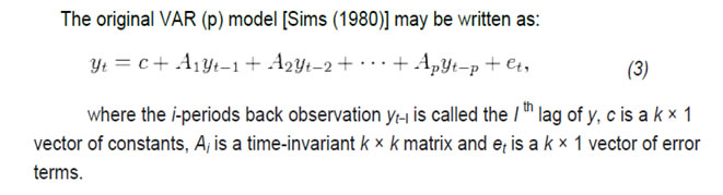 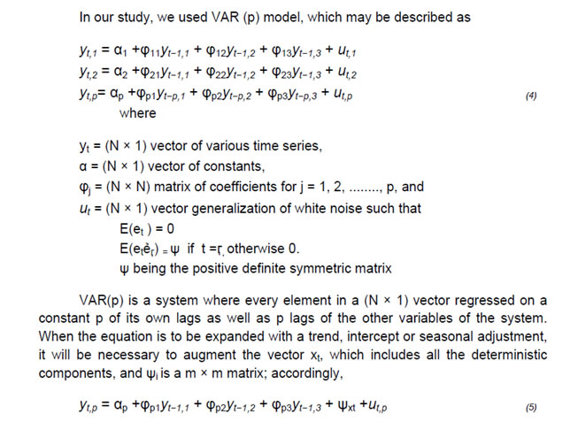 While perusing the literature, it is observed that there is much more common to report functions of the VAR coefficients which are more informative, and have some economic interpretations. Further, the process of choosing the maximum lag p in the VAR model requires special attention because inference is dependent on correctness of the selected lag order. Therefore, studies generally estimate (i) impulse response function, (ii) forecast error variance decompositions and (iii) historical decompositions. Further, it is much more common to report the IRF under VAR framework, which assess the relative contribution of different shocks to fluctuations in variables. Generally, IRF traces the effect of a one-time shock to one of the innovations on current and future values of the endogenous variables. This is normally done with MA(∞) representation of the VAR model. However, the major assumption is that the shocks are independent. We have estimated the IRF under unrestricted VAR framework to assess the response of the yield to sudden shocks or innovation to the system liquidity and the cost of such liquidity, i.e., net system liquidity, repo rate, MSF rate and weighted average call rate. Normality tests are often used for model checking, although normality is not a necessary condition for the validity of the VAR model. However, non-normality of the residuals may indicate other model deficiencies such as nonlinearities or structural changes (Helmut, 2011). Therefore, before estimating the VAR, it would be more appropriate to test the statistical properties of the data used in the empirical analysis. The unit root test has been attempted to ascertain the stationarity of the series. The unit root test reveals that the amount of auction and the residual maturity of the securities are stationary at levels [I(O) series] while other variables are stationary at their first difference [I(1) series] (Table 5). The results are statistically significant at 1 per cent level. While the variables used in the VAR are stationary in their first difference, it means that they are integrated with order I(1). Results As per IRF estimation under the condition of cholesky degrees of freedom adjusted, in case system liquidity is in deficit phase, when a positive shock is given to the net availability of liquidity, the bond yield gradually moves to the reverse direction in the first four period (four weeks) and thereafter, the yield stabilizes at a level lower than the level before the shock is effected (Annex 1). In this scenario, while a shock to repo rate does not stimulate the yield movements much, however, expected increase in repo rate has immediate positive impact on the yield, which increases immediately and thereafter it reverts and stabilizes at the earlier level. The call rate responds positively and the yield increases slowly and stabilizes at an elevated level. In times of surplus liquidity phase, an innovation in liquidity does not impact the yield movement much as the system is already flooded with liquidity. In such a situation, a shock to repo rate has little impact on the yield. However, expected increase in call rate impact the yield significantly and thereafter stabilizes at the earlier level (Annex 2). To study the impact on the yield of different maturities of G-Secs in the primary auctions, the data for the period from November 2008 to February 2014 were segregated according to the residual maturity in three groups, viz., (i) upto 10 years, (ii) above 10 years and upto 20 years and (iii) above 20 years. While estimating the IRF, shocks to the liquidity, repo and call rates impact the bond yield at the desired direction in the maturity bucket of 10-20 years securities whereas yield of securities upto 10 year maturity is impacted by the shock of liquidity and repo rate. Securities having residual maturity of above 20 years, the impact on the yield is significantly low when a shock to the liquidity is effected. This may be due to the fact that the interest on long term investments are being decided mainly by inflation expectations, interest rate scenario and the long term cost of funds. The repo rate has impacted the yield of the G-Secs significantly with all maturities upto 30 years. In case of securities with maturities above 20 years, a shock to call rate impacts the yield after two weeks. In all the three categories of maturity, when a shock is given to the repo rate, the yield responds positively and increases immediately and thereafter stabilizes above the level of the pre-shock period (Annex 3, 4 & 5). It needs to be mentioned that the repo rate has been used as lead indicator, which has direct impact on the yield of the bond. In addition to repo rate shock, expectation of increase in repo rate also impulse the yield to increase and the same is the case with the call rate. However, when the market expects a decrease in call rate, bond yield for shorter maturities has decreased in anticipation. This was evidenced during 2014 when the market was speculating such a decline in call rate as a consequence of reduction in repo rate. When the IRF is estimated with combined liquidity phase (deficit and surplus), the yield does not respond to positive shocks in liquidity. However, the yield responds positively to shocks in marginal standing facility and repo rates. Accordingly, when the rates of repo and MSF are increased, the yield also tends to increase simultaneously. The variance decomposition provides information about the relative importance of each random innovation in affecting the variables in the VAR. Therefore, in addition to the IRF exercise, we attempted the variance decomposition sequence to analyze a compact overview of the dynamic structures of VAR framework. Variance decomposition analysis reveals that positive shocks to liquidity impact the yield of the securities with maturities upto 20 years. However, shock to repo rate affects the yield more significantly in all the maturities and the call rate affects the yield of the securities with maturities over 10 years (Annex 6.1 to 6.5). Overall, though various factors determine the yield of the dated securities of the GoI in the primary auctions, the availability of short term liquidity and the cost of such liquidity also impact the yield significantly. Expected increase in repo rate has significant and immediate impact on the yield. The technical estimates represented by charts and tables are given in Technical Appendix.5. Concluding Observations and Policy Options The main objective of PDM is to ensure that the government’s financing needs and its payment obligations to be met at the lowest possible cost over the medium to longer run, consistent with the prudent degree of rollover risk as also to promote the development of the domestic G-Sec market. The international experience reveals that development of the G-Sec market across the yield curve, broaden the investor base with more retail participation, transparent debt issuance calendar using standardized instruments, market-based mechanisms, sound payment and settlement systems, lower interest rate policy, if inflation expectation is not a threat and enhancement of liquidity to reduce the costs of borrowings are the common lessons. The public debt management in India has clearly traversed from a passive system to a market driven process with developed institutions, varied instruments, intermediaries for market making and well-developed market infrastructure. Market borrowing has emerged as the primary source of financing of GFD of the GoI as well as the sub-national Governments during the recent period. The internal control mechanism has to be strengthened to address the operational risk, legal risk, security breaches, reputational risk, etc., which would otherwise adversely reflect on the debt management structure. Excessive reliance on short-term instruments to take advantage of lower short-term interest rates may lead to increase in rollover risk and possibly increase the debt service costs. Balance sheet risk of the Government should be reduced by issuing debt primarily in long dated, fixed rate and domestic currency securities, which is being reflected in the debt management strategy of India. The holding pattern of government debt shows some reduction in the captive holdings by banks and financial institutions and increase in the relative share of non-banks, reflecting a progressive proliferation of the investor base. Notwithstanding the above, certain issues and challenges remain in the PDM in India such as limited liquidity across the yield curve, which pose challenge for the development of the secondary market; more diversified instruments that may widen the investors participation; increased participation of mid-segment and retail investors to remove narrow investor base; more transparency through release of indicative calendar for SDLs setting out details of issuances, etc. Though the yield on G-Sec is broadly determined by various factors such as expected liquidity risk, repayment risk, economic prosperity and the inflation expectations, however, sudden shocks in the availability of liquidity and the cost of such liquidity are also important factors that determine the yield. Impulse response function under unrestricted VAR framework reveals that, in a deficit liquidity scenario, positive shock in liquidity leads to gradual decline in bond yield, which stabilizes thereafter at a level lower than the level before the shock was effected. While shock to repo rate affects the yield of the securities of all maturities, shock to call rate affects the yield of the securities with residual maturities of 10 to 20 years and lagged effect in the yield is observed in maturities over 20 years. Expectation of increase in repo rate also affects the bond yield positively. Variance decomposition analysis also confirms that shocks to repo rate affect the yield of the securities of all maturities while shocks to liquidity impact the yield of the securities with maturities upto 20 years. In addition, the two mean t-test analysis also corroborate the findings. Overall, the availability of liquidity and the cost of short term liquidity are also important factors that determine the yield along with other factors. A well-balanced approach aimed at addressing the issues and challenges with innovative procedures, policies and appropriate product-mix with efficient market infrastructure would make the PDM structure and strategies more robust. @ Shri L. Lakshmanan and Smt R. Kausaliya are Assistant Adviser and Director of Internal Debt Management Department of Reserve Bank of India. The authors are also thankful to an anonymous referee for his valuable comments on the earlier draft. * Views expressed in the paper are those of authors and not of the Reserve Bank. 1R Gandhi: Sovereign debt management in India: interaction with monetary policy: BIS Papers No XX – 2012 2Revised guidelines for public debt management, World Bank and the IMF, April 1, 2014 Select References:
Technical Appendix Annex 1: Impulse Response of Yield - Liquidity in deficit Mode 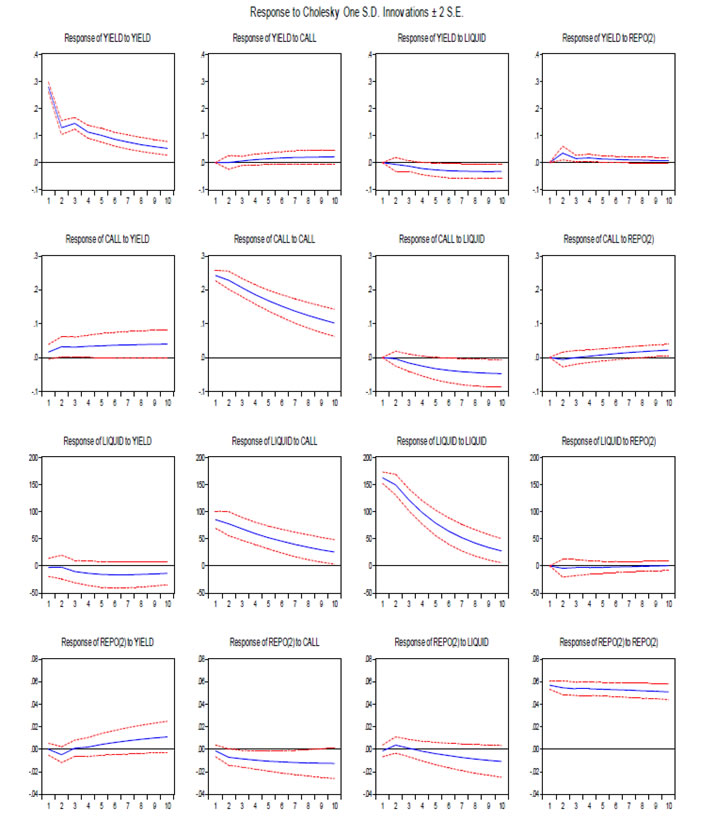 Annex 2: Impulse Response of Yield - Liquidity in Surplus Mode 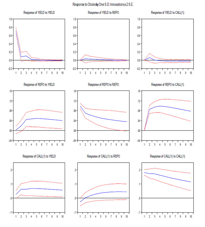 Annex 3: Impulse Response of Yield - Residual Maturity upto 10 years 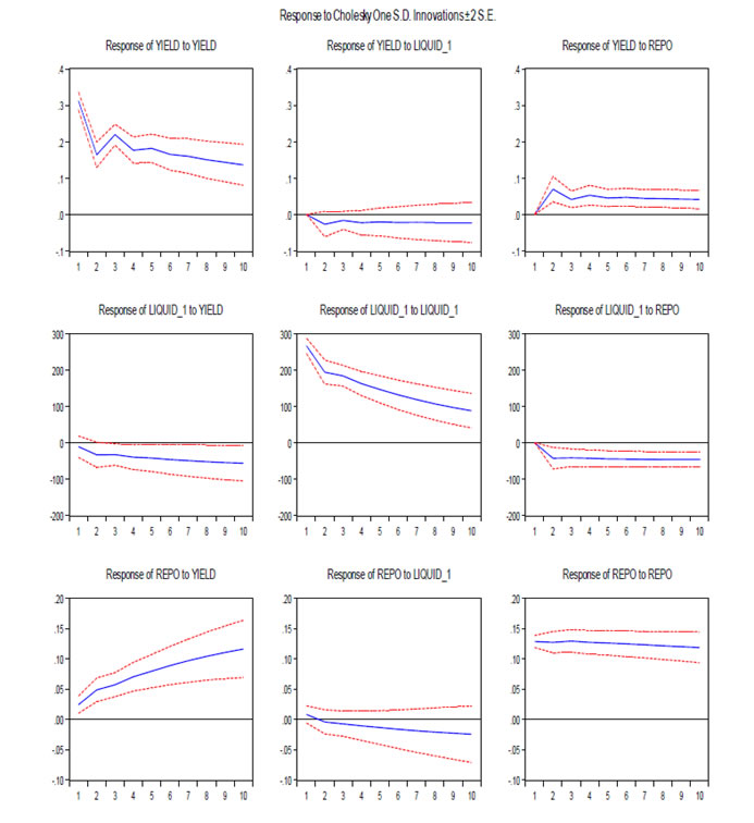 Annex 4: Impulse Response of Yield - Residual Maturity 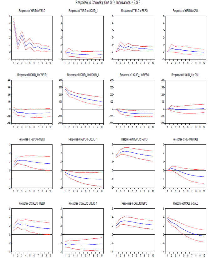 Annex 5: Impulse Response of Yield - Residual Maturity 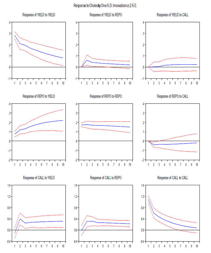
| ||||||||||||||||||||||||||||||||||||||||||||||||||||||||||||||||||||||||||||||||||||||||||||||||||||||||||||||||||||||||||||||||||||||||||||||||||||||||||||||||||||||||||||||||||||||||||||||||||||||||||||||||||||||||||||||||||||||||||||||||||||||||||||||||||||||||||||||||||||||||||||||||||||||||||||||||||||||||||||||||||||||||||||||||||||||||||||||||||||||||||||||||||||||||||||||||||||||||||||||||||||||||||||||||||||||||||||||||||||||||||||||||||||||||||||||||||||||||||||||||||||||||||||||||||||||||||||||||||||||||||||||||||||||||||||||||||||||||||||||||||||||||||||||||||||||||||||||||||||||||||||||||||||||||||||||||||||||||||||||||||||||||||||||||||||||||||||||||||||||||||||||||||||||||||||||||||||||||||||||||||||||||||||||||||||||||||||||||||||||||||||||||||||||||||||||||||||||||||||||||||||||||||||||||||||||||||||||||||||||||||||||||||||||||||||||||||||||

Share this page:


Install the RBI mobile application and get quick access to the latest news!
Scan the QR code to install our app


Page Last Updated on:


